A sufficient optimality condition for delayed state-linear optimal control problems
Ana P. Lemos-Paiao, Cristiana J. Silva, Delfim F. M. Torres

TL;DR
This paper establishes a sufficient optimality condition for delayed state-linear control problems by transforming them into equivalent non-delayed problems, enabling the application of existing theorems.
Contribution
It introduces a novel method to handle delays in state-linear optimal control problems by converting them into non-delayed problems for analysis.
Findings
Proved a sufficient optimality condition for delayed state-linear control problems.
Demonstrated the method with an illustrative example.
Extended the applicability of known theorems to delayed systems.
Abstract
We give answer to an open question by proving a sufficient optimality condition for state-linear optimal control problems with time delays in state and control variables. In the proof of our main result, we transform a delayed state-linear optimal control problem to an equivalent non-delayed problem. This allows us to use a well-known theorem that ensures a sufficient optimality condition for non-delayed state-linear optimal control problems. An example is given in order to illustrate the obtained result.
Click any figure to enlarge with its caption.
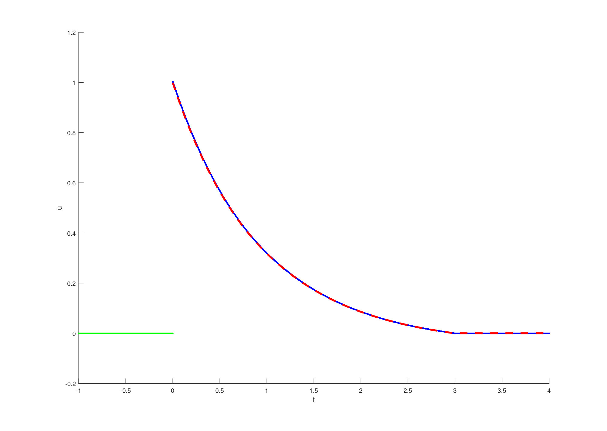 Figure 1
 Figure 2
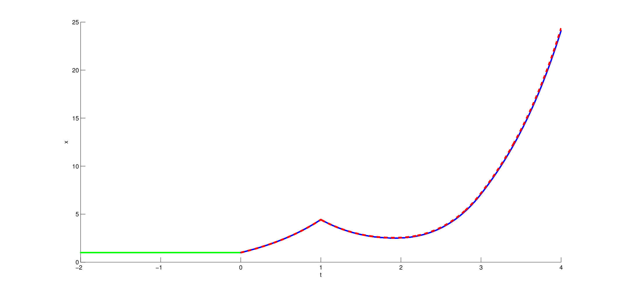 Figure 3
Peer Reviews
No public reviews on file for this paper yet. If you reviewed it on a platform where reviews are public (OpenReview, ICLR, NeurIPS, ICML), you can paste yours below so the community can read it here.
Videos
No videos yet. Explain this paper in a talk, walkthrough, or lecture? Add one.
A sufficient optimality
condition for delayed state-linear optimal control problems
Abstract.
We give answer to an open question by proving a sufficient optimality condition for state-linear optimal control problems with time delays in state and control variables. In the proof of our main result, we transform a delayed state-linear optimal control problem to an equivalent non-delayed problem. This allows us to use a well-known theorem that ensures a sufficient optimality condition for non-delayed state-linear optimal control problems. An example is given in order to illustrate the obtained result.
Key words and phrases:
Delayed optimal control problems, delayed state-linear control systems, time delays in state and control variables, sufficient optimality condition, augmented problem.
1991 Mathematics Subject Classification:
Primary: 49K15; Secondary: 34H99
This work is part of first author’s Ph.D., which is carried out at the University of Aveiro.
∗Corresponding author: Delfim F. M. Torres ([email protected])
Ana P. Lemos-Paião, Cristiana J. Silva and Delfim F. M. Torres∗
Center for Research and Development in Mathematics and Applications (CIDMA)
Department of Mathematics, University of Aveiro, 3810-193 Aveiro, Portugal
1. Introduction
Time delays occur in many dynamical systems such as biological, chemical, mechanical and economical systems (see, e.g., [3, 11, 16, 27, 44, 48, 49, 50, 51]). Dynamic systems with time delays, in both state and control variables, play an important role in the modelling of real-life phenomena in various fields of applications [15, 16]. For instance, in [42] the incubation and pharmacological delays are modelled through the introduction of time delays in both state and control variables. In [46], Silva, Maurer and Torres introduce time delays in the state and control variables for tuberculosis modelling. They represent the time delay on the diagnosis and commencement of treatment of individuals with active tuberculosis infection and the delays on the treatment of persistent latent individuals, due to clinical and patient reasons. There is a vast literature on delayed optimal control problems, also called retarded, time-lag, or hereditary optimal control problems. See, e.g., [2, 4, 13, 15, 18, 36] and references cited therein.
Delayed linear differential systems have also been investigated, their importance being recognized both from a theoretical and practical points of view. For instance, in [13] Friedman considers linear hereditary processes and apply to them Pontryagin’s method, deriving necessary optimality conditions as well as existence and uniqueness results. Analogously, in [36] linear delayed differential equations and optimal control problems involving this kind of systems are studied. Since these first works, many researchers have devoted their attention to linear quadratic optimal control problems with time delays, see, e.g., [7, 10, 12, 26, 37]. It turns out that for linear quadratic delayed optimal control problems it is possible to provide an explicit formula for the optimal controls [7, 26, 37].
Optimal control problems with a differential system that is linear both in state and control variables have been studied in [7, 9, 10, 12, 26, 28, 29, 31, 35, 37]. In [10, 28, 37], the system is delayed with respect to state and control variables. In [9, 35], the system only considers delays in the state variable. Chyung and Lee derive necessary and sufficient optimality conditions in [9] while Oǧuztöreli only proves necessary conditions [35]. Certain necessary conditions analysed by Chyung and Lee in [9] have been already derived in [23, 40, 41]. However, the system considered in [9] is different from the previously studied hereditary systems, which do not require a initial function of state. In [12], Eller et al. derive a sufficient condition for a control to be optimal for certain problems with time delay. The problems studied by Eller et al. and Khellat, respectively in [12] and [26], consider only one constant lag in the state. The research done by Lee in [31] is different from ours, because in [31] the aim is to minimize a cost functional, which does not consider delays, subject to a differential system that is linear in state and control variables, and to another constraint. In their differential system, the state variable depends on a constant and fixed delay and the control variable depends on a constant lag, which is not specified a priori. Note that the differential system of the problem considered in [29] is similar to the one of [31]. Although Banks has studied non-linear delayed problems without lags in the control, he has also analyzed problems that are linear and delayed with respect to control [2]. Recently, Cacace et al. studied optimal control problems that involve linear differential systems with variable delays only in the control [7]. The problems analyzed in the present paper are different from those considered in the mentioned works, because here the problems involve differential systems that are linear with respect to state, but not with respect to the control. Furthermore, we consider a constant lag in the state and another one in the control. These two delays are in general not equal.
In [20], Hughes firstly consider variational problems with only one constant lag and derive various necessary and a sufficient optimality condition for them. The variational problems in [20] can easily be transformed to control problems with only one constant delay (see, e.g., [34, p. 53–54]). Hughes also investigate an optimality condition for a control problem with a constant delay, which is the same for state and control. Therefore, the problems investigated in [20] are different from the problems studied by us, because in the present paper the delay of state is not necessarily equal to the delay of control. The problems analyzed by Chan and Yung [8] and by Sabbagh [43] are similar to the first problems studied by Hughes in [20]. So, for the same reason, the problems investigated in [8, 43] are different from ours. The problems considered in [20, 43] are also considered in [38] by Palm and Schmitendorf. For such problems, they derive two conjugate-point conditions, which are not equivalent. Note that their conditions are only necessary and do not give a set of sufficient conditions [38].
In [22], Jacobs and Kao investigate delayed problems that consist to minimize a cost functional without delays subject to a differential system defined by a non-linear function with a delay in state and another one in the control. Similar to our case, these delays do not have to be equal. In contrast, our cost functional contains also time delays, therefore being more general than the one considered in [22]. Jacobs and Kao transform the problem using a Lagrange-multiplier technique and prove a regularity result in the form of a controllability condition, as well as some necessary optimality conditions. Then, in some special restricted cases, they prove existence, uniqueness and sufficient conditions. Such restricted problems consider a differential system that is linear in state and in control variables. Thus, the sufficient conditions of [22] are derived for problems that are less general than ours.
The delayed optimal control problems analyzed by Schmitendorf in [45] have a cost functional and a differential system that are more general than ours. However, in [45] the control takes its values in all while in the present paper the control values belong to a set , . In [32], Lee and Yung study a problem that is similar to the one considered in [45], where the control belongs to a subset of , as we consider here. First and second-order sufficient conditions are shown in [32]. Nevertheless, the conditions of [32] are not constructive and practical for the computation of the optimal solution. Indeed, as hypothesis, it is assumed existence of a symmetric matrix under some conditions, for which is not given a method to calculate its expression. Another similar problem to our is studied by Bokov in [6], in order to arise a necessary optimality condition in an explicit form. Moreover, a solution to the problem with infinite time horizon is given in [6]. In contrast, in the present paper we are interested to derive sufficient optimality conditions. As it is well known, and as Hwang and Bien write in [21], many investigations have directed their efforts to seek sufficient conditions for control problems with delays: see, e.g., [9, 12, 20, 22, 32, 45]. In [21], Hwang and Bien prove a sufficient condition for problems involving a differential affine time-delay system with the same lag for the state and the control. Thus, the differential system considered in the present article is obviously more general. In 1996, Lee and Yung derived various first and second-order sufficient conditions for non-linear optimal control problems, with only a constant delay in the state, and considering functions that do not have to be convex [30]. As in [8, 32], second-order sufficient conditions are shown to be related to the existence of solutions of a Riccati-type matrix differential inequality.
Optimal control problems with multiple delays have also been investigated. In [18], Halanay derive necessary conditions for some optimal control problems with various time lags in state and control variables, using the abstract multiplier rule of Hestenes [19]. In [18], all delays related to state are equal to each other and the same happens with the delays associated to the control. Note that the results of [13, 23] are obtained as particular cases of problems considered in [18]. Later, in 1973, a necessary condition is derived for an optimal control problem that involves multiple constant lags only in the control. This delayed dependence occurs both in the cost functional and in the differential system, which is defined by a non-linear function [47]. In [25], Kharatishvili and Tadumadze prove the existence of an optimal solution and a necessary condition for optimal control systems with multiple variable time lags in the state and multiple variable commensurable time delays in the control. Later, an optimal control problem where the state variable is solution of an integral equation with multiple delays, both for state and control variables, is studied by Bakke in [1]. Furthermore, necessary conditions and Hamilton–Jacobi equations are derived. In 2013, Boccia, Falugi, Maurer and Vinter derived necessary conditions for a free end-time optimal control problem subject to a non-linear differential system with multiple delays in the state [4]. The control variable is not influenced by time lags in [4]. Recently, in 2017, Boccia and Vinter obtained necessary conditions for a fixed end-time problem with a constant and unique delay for all variables, as well as free end-time problems without control delays [5].
As Guinn wrote, the classical methods of obtaining necessary conditions for retarded optimal control problems (used, for instance, by Halanay in [18], Kharatishvili in [24] and Oǧuztöreli in [36]) require complicated and extensive proofs [17] (see, e.g., [2, 13, 18, 24, 36]). In , Guinn proposed a method whereby we can reduce some specific time-lag optimal control problems to equivalent and augmented optimal control problems without delays [17]. By reducing delayed optimal control problems into non-delayed ones, we can then use well-known theorems applicable for optimal control problems without delays to derive desired optimality conditions for delayed problems [17]. In [17], Guinn study specific optimal control problems with a constant delay in state and control variables. These two delays are equal. Later, in , Göllmann, Kern and Maurer studied optimal control problems with a constant delay in state and control variables subject to mixed control-state inequality constraints [15]. In that research, the delays do not have to be equal. For technical reasons, the authors need to assume that the ratio between these two time delays is a rational number [15]. In [15], the method used by Guinn in [17] is generalized and, consequently, a non-delayed optimal control problem is obtained again. Pontryagin’s Minimum Principle, for non-delayed control problems with mixed state-control constraints, is used and first-order necessary optimality conditions are derived for retarded problems [15]. Furthermore, Göllmann, Kern and Maurer discuss the Euler discretization for the retarded problem and some analytical examples versus correspondent numerical solutions are given. Later, in 2014, Göllmann and Maurer generalized the research mentioned before, by studying optimal control problems with multiple and constant time delays in state and control, involving mixed state-control inequality constraints [16]. Again, necessary optimality conditions are derived [16]. Note that the works [15, 16, 17, 18] consider non-linear delayed differential systems.
In the present paper, we consider optimal control problems that consist to minimize a delayed non-linear cost functional subject to a delayed differential system that is linear with respect to state, but not with respect to control. The delay in the state is the same for the cost functional and for the differential system. The same happens with the time lag of the control variable. We derive a sufficient optimality condition for this type of problems. Note that the cost functional does not have to be quadratic, but it satisfies some continuity and convexity assumptions. To the best of our knowledge, this gives answer to an open question. Note that the constant delays on the state and control variables do not have to be equal, but we ensure the commensurability assumption between state and control delays, similarly to Göllmann, Kern and Maurer in [15]. Indeed, we follow the approach of [15] and Guinn [17], that is, we transform the delayed optimal control problem into an equivalent non-delayed optimal control problem and then apply a classical sufficient optimality condition [33, p. 340–343].
The paper is organized as follows. In Section 2, we define the optimal control problem without delays for which the sufficient optimality condition [33, p. 340–343] holds. In Section 3, we define our retarded optimal control problem with constant time delays in state and control variables. Then, in Section 4, we prove a sufficient optimality condition for the problem stated in Section 3. A concrete example is solved in detail in Section 5, with the purpose to illustrate our main result. We end with some conclusions in Section 6.
2. Non-delayed state-linear optimal control problem
We begin by defining a non-delayed state-linear optimal control problem and recall a well-known sufficient optimality result for such class of problems.
Consider the non-delayed state-linear optimal control problem (LP) which consists to
[TABLE]
subject to the control system in
[TABLE]
with initial boundary condition
[TABLE]
and final boundary condition ; where is a closed convex set, , and is a real matrix, . Functions , and are assumed to be continuous for all .
Notation**.**
Along the text we use the notation to denote the partial derivative of a certain function with respect to its th argument. For example, .
Definition 2.1**.**
An admissible process to (LP) is given by a pair of functions that satisfies conditions (2) and (3).
The following theorem gives a sufficient optimality condition for problem (LP).
Theorem 2.2** (See Theorem 5, Section 5.2 of [33]).**
Consider problem (LP) and assume that
- (1)
functions , , , and are continuous for all ; 2. (2)
* is a convex function in for each fixed ;* 3. (3)
for almost all , is a control with response that satisfies the maximality condition
[TABLE]
where
[TABLE]
and is any nontrivial solution of the adjoint system
[TABLE]
satisfying the transversality condition that ensures that is an inward normal vector of at the boundary point .
Then, is an optimal control that leads to the minimal cost .
Remark 1**.**
Note that if , then the transversality condition of Theorem 2.2 is vacuous, because has a single point. If , then .
3. Delayed state-linear optimal control problem
In this paper we are interested in state-linear optimal control problems with discrete time delays in the state variables and in the control variables , . The delayed state-linear optimal control problem () consists in
[TABLE]
subject to the delayed differential system
[TABLE]
with the following initial functions
[TABLE]
where for each and for each .
Definition 3.1**.**
An admissible process to problem () is given by a pair of functions that satisfies conditions (4)–(5).
4. Main Result
In what follows, we assume that the time delays and respect the following commensurability assumption.
Assumption 4.1** (Commensurability assumption).**
We consider not simultaneously equal to zero and commensurable, that is,
[TABLE]
and
[TABLE]
Remark 2**.**
The commensurability assumption holds for any couple of rational numbers for which at least one number is nonzero [15].
Theorem 4.2**.**
Consider problem () and assume that
- (1)
functions , , , , , , and are continuous for all their arguments; 2. (2)
* is a convex function in for each ;* 3. (3)
for almost all , is a control with response that satisfies the maximality condition
[TABLE]
where
[TABLE]
for , and is any nontrivial solution of the adjoint system
[TABLE]
that satisfies the transversality condition .
Then, is an optimal control that leads to the minimal cost .
Proof.
We transform the delayed state-linear optimal control problem () into an equivalent non-delayed state-linear optimal control (LP) type problem, using the approach of [15, 17], and then we apply Theorem 2.2. Without loss of generality, we assume the first case of Assumption 4.1, that is, for and . Consequently, there exist such that
[TABLE]
Thus, let us divide the interval into subintervals of amplitude . We can note that
[TABLE]
Furthermore, we also assume that
[TABLE]
with .
Remark 3**.**
If is not a multiple of (), then we can study problem () for , where is the smallest multiple of , which is greater than . Thus, we also study problem () for , because .
For and for , we define new variables
[TABLE]
In Figure 1, we can observe a simple scheme for the new state variables. The idea is similar for the new control variables. We transform the delayed state-linear problem () into an equivalent non-delayed state-linear problem , which consists to
[TABLE]
subject to the non-delayed differential system
[TABLE]
, and to the initial functions
[TABLE]
Consider that
[TABLE]
Observe that the dimensions of , , and are , , and , respectively. Note also that and represent optimization variables and and not. We know, a priori, the expressions of , , and , . Let us write the objective function expressed in (8) as a function of the type presented in (1):
[TABLE]
As , , and are known, . Similarly, we can write . Consequently,
[TABLE]
In order to apply Theorem 2.2, we have to write the set of constraints
[TABLE]
, in the form
[TABLE]
For , consider that . Thus, we have
[TABLE]
and
[TABLE]
Note that , and have dimension . Concluding, we have
[TABLE]
Now, we write the sum of the third and fourth terms of (9) as a function of and . Thus,
[TABLE]
As and are known, we have that
[TABLE]
Therefore, we have the set of constraints (9) in form (10). To apply Theorem 2.2, we have to ensure that
- (1)
, , , and are continuous for all ; 2. (2)
is a convex function in for each fixed ; 3. (3)
is a control with response that satisfies the maximality condition
[TABLE]
for almost all . Note that and is any nontrivial solution of the adjoint system
[TABLE]
such that is an inward normal vector of the closed convex set
[TABLE]
at the boundary point for .
Thus, will be an optimal control that leads us to the minimal cost . From now on, we are going to analyze each hypothesis of Theorem 4.2.
-
(1)
-
(a)
We have that
[TABLE]
By hypothesis, function is continuous with respect to all its arguments. Then, is continuous for all . 2. (b)
Having in mind that (see (7)), that is, , then
[TABLE]
So, for , we obtain
[TABLE]
For and , we conclude that
[TABLE]
For we have
[TABLE]
As and , we obtain
[TABLE]
For each , there exists such that
[TABLE]
Thus, let us define as being . Consequently,
[TABLE]
Since is continuous for all and function is continuous for all , then is continuous for all . 3. (c)
We have that
[TABLE]
By hypothesis, function is continuous for all . Then, is continuous for all . 4. (d)
We know that . As and are continuous for all and and are depending on for and on for , then is continuous for all . 5. (e)
Let us define function by
[TABLE]
for all . We have already defined
[TABLE]
The matrix is depending on the matrix for . As is continuous in the interval , then
[TABLE]
is continuous for all . Function is continuous if, for each , the functions and are continuous for all , respectively. We know that and
[TABLE]
. Moreover, as and are continuous for all , is continuous for all . 2. (2)
As we know,
[TABLE]
for and is convex in for each . Then, is a convex function in for each fixed . 3. (3)
If is a control with response that satisfies the maximality condition
[TABLE]
for almost all , then
[TABLE]
for almost all and for all admissible . If we consider that , then we have that
[TABLE]
and
[TABLE]
which implies . As equation (11) is verified for all admissible , we can choose an admissible variable such that
[TABLE]
where is an admissible control of problem (). So, using inequality (11) and considering , we have that
[TABLE]
As the last sums of both sides of previous inequality are equal, we obtain
[TABLE]
Due to the choice of , , some terms of the left-hand side of inequality (12) cancel with other terms of the right-hand side. Let us analyze the sums when we only consider the indexes of set . For the first member, we have
[TABLE]
while for the second we obtain
[TABLE]
Only the terms associated to the indexes are different. Therefore, inequality (12) is equivalent to
[TABLE]
For , we know that , if . Thus, by the above inequality, it follows that
[TABLE]
As and , then
[TABLE]
Consequently, we have that
[TABLE]
As some terms cancel, we obtain
[TABLE]
Using relations and , we have that
[TABLE]
Attending to the definition of , , the inequality (13) is equivalent to the maximality condition (6) of Theorem 4.2. Furthermore, we cannot forget that is any nontrivial solution of the adjoint system
[TABLE]
that satisfies the transversality condition (see Remark 4)
[TABLE]
As we know,
[TABLE]
and where has dimension for all . Consequently, by the adjoint system (14), we can write that
[TABLE]
Furthermore, as , we conclude that
[TABLE]
By equation (15),
[TABLE]
As , we obtain the transversality condition
[TABLE]
With conditions (13), (16) and (17), we obtain item of Theorem 4.2.
The proof is complete. ∎
Remark 4**.**
We can note that: (i) problems () and () are equivalent; (ii) the augmented and non-delayed problem () is defined for . Even more, we can solve problem () by solving sub-problems, each one with respect to each subinterval of with amplitude . Then, we can concatenate the respective optimal solutions in order to obtain an optimal solution of (). Thus, we can solve problem () by solving augmented and non-delayed sub-problems () associated to problem (), with . For , the th augmented and non-delayed sub-problem () consists to minimize
[TABLE]
subject to
[TABLE]
for . Theorem 2.2 can be applied and we can find an optimal pair in the interval of time that provides an optimal solution in the interval of time . The set has a single point. So, is an inward normal vector of at the boundary point (recall Remark 1). The last augmented and non-delayed sub-problem () consists to minimize
[TABLE]
subject to
[TABLE]
for . Again, Theorem 2.2 can be applied and we can find an optimal pair in interval of time that provides an optimal solution in the interval of time . As , then by Theorem 2.2 .
5. An illustrative example
Let us consider problem given by
[TABLE]
where for each . Thus, we have that , , , , , , , , and . Note that our functions respect hypothesis and of Theorem 4.2. Let be an admissible control of problem () and let us maximize function
[TABLE]
with respect to . We obtain
[TABLE]
for and for . Furthermore, we know that is any nontrivial solution of
[TABLE]
that satisfies the transversality condition . The adjoint system is given by
[TABLE]
For , the solution of differential equation
[TABLE]
is given by
[TABLE]
Knowing , , and attending to the continuity of function for all , we can determine for solving the differential equation
[TABLE]
for . Therefore,
[TABLE]
and, consequently, the solution of the adjoint system (18) is given by
[TABLE]
So, the control is given by
[TABLE]
Knowing the control, we can determine the state by solving the differential equation
[TABLE]
The state solution is
[TABLE]
Such analytical expressions can be obtained with the help of a modern computer algebra system. We have used Mathematica. In Figures 2 and 3, we observe that the numerical solutions for control and state, obtained using AMPL [14] and IPOPT [39], are in agreement with their analytical solutions, given by (19) and (20), respectively. The numerical solutions were obtained using Euler’s forward difference method in AMPL and IPOPT, dividing the interval of time into 2000 subintervals. The minimal cost is
[TABLE]
6. Conclusion
We considered a delayed state-linear optimal control problem. We proved a sufficient optimality condition for problems with delays in both state and control variables. The proof is based on the transformation of the delayed state-linear optimal control problem into a non-delayed one, following the approach proposed in [17] and used in [15]. Analogously to [15], we ensure the commensurability assumption between the, possibly different, state and control delays. An example is provided, which illustrates the usefulness of obtained sufficient optimality condition.
Acknowledgements
This research was supported by the Portuguese Foundation for Science and Technology (FCT) within projects UID/MAT/04106/2019 (CIDMA) and PTDC/EEI-AUT/2933/2014 (TOCCATA), funded by Project 3599 – Promover a Produção Científica e Desenvolvimento Tecnológico e a Constituição de Redes Temáticas and FEDER funds through COMPETE 2020, Programa Operacional Competitividade e Internacionalização (POCI). Lemos-Paião is also supported by the Ph.D. fellowship PD/BD/114184/2016; Silva by national funds (OE), through FCT, I.P., in the scope of the framework contract foreseen in the numbers 4, 5 and 6 of the article 23, of the Decree-Law 57/2016, of August 29, changed by Law 57/2017, of July 19. The authors are very grateful to a referee for carefully reading of their manuscript and for several constructive remarks.
The reference list from the paper itself. Each links out to its DOI / PubMed record.
- 1[1] (MR 0608894) [10.1007/BF 00935177] V. L. Bakke, Optimal fields for problems with delays, J. Optim. Theory Appl. 33 (1981), 69–84.
- 2[2] (MR 0231007) [10.1137/0306002] H. T. Banks, Necessary conditions for control problems with variable time lags, SIAM J. Control 6 (1968), 9–47.
- 3[3] (MR 3542538) [10.1016/j.amc.2016.07.009] E. B. M. Bashier and K. C. Patidar, Optimal control of an epidemiological model with multiple time delays, Appl. Math. Comput. 292 (2017), 47–56.
- 4[4] [10.1109/CDC.2013.6759934] A. Boccia, P. Falugi, H. Maurer and R. Vinter, Free time optimal control problems with time delays, 52nd IEEE Conference on Decision and Control (2013), 520–525.
- 5[5] (MR 3702857) [10.1137/16M 1085474] A. Boccia and R. B. Vinter, The maximum principle for optimal control problems with time delays, SIAM J. Control Optim. 55 (2017), 2905–2935.
- 6[6] (MR 2745102) [10.1007/s 10958-011-0208-y] G. V. Bokov, Pontryagin’s maximum principle of optimal control problems with time-delay, J. Math. Sci. (N. Y.) 172 (2011), 623–634.
- 7[7] (MR 3459591) [10.1016/j.sysconle.2015.12.003] F. Cacace, F. Conte, A. Germani and G. Palombo, Optimal control of linear systems with large and variable input delays, Systems Control Lett. 89 (2016), 1–7.
- 8[8] (MR 1202585) [10.1007/BF 00952825] W. L. Chan and S. P. Yung, Sufficient conditions for variational problems with delayed argument, J. Optim. Theory Appl. 76 (1993), 131–144.