Analyzing a Maximum Principle for Finite Horizon State Constrained Problems via Parametric Examples. Part 1: Problems with Unilateral State Constraints | Tomesphere
arXiv:1901.03794·math.OC·January 15, 2019
Analyzing a Maximum Principle for Finite Horizon State Constrained Problems via Parametric Examples. Part 1: Problems with Unilateral State Constraints
This paper examines the maximum principle for finite horizon state constrained optimal control problems using parametric examples, focusing on problems with unilateral constraints to deepen understanding and illustrate applications in economic growth models.
Contribution
It provides a detailed analysis of the maximum principle via parametric examples with unilateral constraints, linking theoretical conditions to economic growth models.
Findings
01
Establishes solution existence using Filippov's theorem.
02
Analyzes the maximum principle as a necessary condition.
03
Serves as a prototype for economic optimal growth models.
Abstract
In the present paper, the maximum principle for finite horizon state constrained problems from the book by R. Vinter [\textit{Optimal Control}, Birkh\"auser, Boston, 2000; Theorem~9.3.1] is analyzed via parametric examples. The latter has origin in a recent paper by V.~Basco, P.~Cannarsa, and H.~Frankowska, and resembles the optimal growth problem in mathematical economics. The solution existence of these parametric examples is established by invoking Filippov's existence theorem for Mayer problems. Since the maximum principle is only a necessary condition for local optimal processes, a large amount of additional investigations is needed to obtain a comprehensive synthesis of finitely many processes suspected for being local minimizers. Our analysis not only helps to understand the principle in depth, but also serves as a sample of applying it to meaningful prototypes of economic…
No public reviews on file for this paper yet. If you reviewed it on a platform where reviews are public (OpenReview, ICLR, NeurIPS, ICML), you can paste yours below so the community can read it here.
Videos
No videos yet. Explain this paper in a talk, walkthrough, or lecture? Add one.
Taxonomy
TopicsAerospace Engineering and Control Systems · Optimization and Variational Analysis · Spacecraft Dynamics and Control
Full text
Analyzing a Maximum Principle for Finite Horizon State Constrained Problems via Parametric Examples. Part 1: Problems with Unilateral State Constraints111Financial supports from several research projects in Taiwan and Vietnam are gratefully acknowledged.
V.T. Huong222Institute of Mathematics, Vietnam Academy of Science and Technology, 18 Hoang
Quoc Viet, Hanoi 10307, Vietnam; email: [email protected]; [email protected]., J.-C. Yao333Center for General Education, China Medical University,
Taichung 40402, Taiwan; Email: [email protected], and N.D. Yen444Institute
of Mathematics, Vietnam Academy of Science and Technology, 18 Hoang
Quoc Viet, Hanoi 10307, Vietnam; email: [email protected].
(Dedicated to Professor Do Sang Kim on the occasion of his 65th birthday)
Abstract. In the present paper, the maximum principle for finite horizon state constrained problems from the book by R. Vinter [Optimal Control, Birkhäuser, Boston, 2000; Theorem 9.3.1] is analyzed via parametric examples. The latter has origin in a recent paper by V. Basco, P. Cannarsa, and H. Frankowska, and resembles the optimal growth problem in mathematical economics. The solution existence of these parametric examples is established by invoking Filippov’s existence theorem for Mayer problems. Since the maximum principle is only a necessary condition for local optimal processes, a large amount of additional investigations is needed to obtain a comprehensive synthesis of finitely many processes suspected for being local minimizers. Our analysis not only helps to understand the principle in depth, but also serves as a sample of applying it to meaningful prototypes of economic optimal growth models. Problems with unilateral state constraints are studied in Part 1 of the paper. Problems with bilateral state constraints will be addressed in Part 2.
Keywords: Finite horizon optimal control problem, state constraint, maximum principle, solution existence theorem, function of bounded variation, Borel measurable function, Lebesgue-Stieltjes integral.
It is well known that optimal control problems with state constraints are models of importance, but one usually faces with a lot of difficulties in analyzing them. These models have been considered since the early days of the optimal control theory. For instance, the whole Chapter VI of the classical work [12, pp. 257–316] is devoted to problems with restricted phase coordinates. There are various forms of the maximum principle for optimal control problems with state constraints; see, e.g., [4], where the relations between several forms are shown and a series of numerical illustrative examples have been solved.
To deal with state constraints, one has to use functions of bounded variation, Borel measurable functions, Lebesgue-Stieltjes integral, nonnegative measures on the σ−algebra of the Borel sets, the Riesz Representation Theorem for the space of continuous functions, and so on.
By using the maximum principle presented in [3, pp. 233–254], Phu [10, 11] has proposed an ingenious method called the method of region analysis to solve several classes of optimal control problems with one state and one control variable, which have both state and control constraints. Minimization problems of the Lagrange type were considered by the author and, among other things, it was assumed that integrand of the objective function is strictly convex with respect to the control variable. To be more precise, the author considered regular problems, i.e., the optimal control problems where the Pontryagin function is strictly convex with respect to the control variable.
In the present paper, the maximum principle for finite horizon state constrained problems from the book by Vinter [14, Theorem 9.3.1] is analyzed via parametric examples. The latter has origin in a recent paper by Basco, Cannarsa, and Frankowska [1, Example 1], and resembles the optimal growth problem in mathematical economics (see, e.g., [13, pp. 617–625]). The solution existence of these parametric examples, which are irregular optimal control problems in the sense of Phu [10, 11], is established by invoking Filippov’s existence theorem for Mayer problems [2, Theorem 9.2.i and Section 9.4]. Since the maximum principle is only a necessary condition for local optimal processes, a large amount of additional investigations is needed to obtain a comprehensive synthesis of finitely many processes suspected for being local minimizers. Our analysis not only helps to understand the principle in depth, but also serves as a sample of applying it to meaningful prototypes of economic optimal growth models.
Note that the maximum principle for finite horizon state constrained problems in [14, Chapter 9] covers many known ones for smooth problems and allows us to deal with nonsmooth problems by using the Mordukhovich normal cone and the Mordukhovich subdifferential [7, 8, 9], which are also called the limiting normal cone and the limiting subdifferential. This principle is a necessary optimality condition which asserts the existence of a multipliers set (p,μ,ν,γ) consisting of an absolutely continuous functionp, a function of bounded variationμ, a Borel measurable functionν, and a real numberγ≥0, where (p,μ,γ)=(0,0,0), such that the four conditions (i)–(iv) in Theorem 2.1 below are satisfied. The relationships between these conditions are worthy a detailed analysis. We will present such an analysis via three parametric examples of optimal control problems of the Langrange type, which have five parameters (λ,a,x0,t0,T), where λ>0 appears in the description of the objective function, a>0 appears in the differential equation, x0 is the initial value, t0 is the initial time, and T is the terminal time. Observe that, in Example 1 of [1], T=∞, x0 and t0 are fixed. Problems with unilateral state constraints are studied in Part 1 of the paper. Problems with bilateral state constraints will be addressed in Part 2.
This Part 1 is organized as follows. Section 2 presents some background materials including the above-mentioned maximum principle and Filippov’s existence theorem for Mayer problems. Control problems without state constraints are considered in Section 3, while control problems with unilateral state constraints are studied in Section 4. Some concluding remarks are given in Section 5.
2 Background Materials
In this section, we give some notations, definitions, and results that will be used repeatedly in the sequel.
2.1 Notations and Definitions
The symbol IR (resp., IN) denotes the set of real numbers (resp., the set of positive integers). The norm in the n-dimensional Euclidean space IRn is denoted by ∥.∥. For a subset C⊂IRn, we abbreviate its convex hull to \mboxcoC. For a set-valued map F:IRn⇉IRm, we call the set gphF:={(x,y)∈IRn×IRm:y∈F(x)} the graph of F.
Let Ω⊂IRn be a closed set and vˉ∈Ω. The Fréchet normal cone (also called the prenormal
cone, or the regular normal cone) to
Ω⊂IRn at vˉ is given by
[TABLE]
where
vΩvˉ means v→vˉ with v∈Ω. The Mordukhovich (or limiting) normal cone to Ω at vˉ is defined by
[TABLE]
Given an extended real-valued function φ:IRn→IR∪{−∞,+∞}, one defines the epigraph of φ by \mboxepiφ={(x,μ)∈IRn×IR:μ≥φ(x)}. The Mordukhovich subdifferential (or limiting subdifferential) of φ at xˉ∈IRn with ∣φ(xˉ)∣<∞ is defined by
[TABLE]
If ∣φ(x)∣=∞, then one puts ∂φ(xˉ)=∅.
The reader is referred to [7, Chapter 1] and [9, Chapter 1] for comprehensive treatments of the Fréchet normal cone, the limiting normal cone, the limiting subdifferential, and the related calculus rules.
For a given segment [t0,T] of the real line, we denote the σ-algebra of its Lebesgue measurable subsets (resp., the σ-algebra of its Borel measurable subsets) by L (resp., B). The Sobolev space W1,1([t0,T],IRn) is the linear space of the absolutely continuous functions x:[t0,T]→IRn endowed with the norm ∥x∥W1,1=∥x(t0)∥+∫t0T∥x˙(t)∥dt (see, e.g., [5, p. 21] for this and another equivalent norm).
As in [14, p. 321], we consider the following finite horizon optimal control problem of the Mayer type, denoted by M,
[TABLE]
over x∈W1,1([t0,T],IRn) and measurable functions u:[t0,T]→IRm satisfying
[TABLE]
where [t0,T] is a given interval, g:IRn×IRn→IR, f:[t0,T]×IRn×IRm→IRn, and h:[t0,T]×IRn→IR are given functions, C⊂IRn×IRn is a closed set, and U:[t0,T]⇉IRm is a set-valued map.
A measurable function u:[t0,T]→IRm satisfying u(t)∈U(t) a.e. t∈[t0,T] is called a control function. A process(x,u) consists of a control function u and an arc x∈W1,1([t0,T];IRn) that is a solution to the differential equation in (2.2). A state trajectoryx is the first component of some process (x,u). A process (x,u) is called feasible if the state trajectory satisfies the endpoint constraint(x(t0),x(T))∈C and the state constrainth(t,x(t))≤0 for all t∈[t0,T].
Due to the appearance of the state constraint, the problem M in (2.1)–(2.2) is said to be an optimal control problem with state constraints. But, if the inequality h(t,x(t))≤0 is fulfilled for every (t,x(t)) with t∈[t0,T] and x∈W1,1([t0,T];IRn) (for example, when h is constant function having a fixed nonpositive value), i.e., the condition h(t,x(t))≤0 for all t∈[t0,T] can be removed from (2.2), then one says that M an optimal control problem without state constraints.
The HamiltonianH:[t0,T]×IRn×IRn×IRm→IR of (2.2) is defined by
[TABLE]
Definition 2.1**.**
A feasible process (xˉ,uˉ) is called a W1,1local minimizer for M if there exists δ>0 such that g(xˉ(t0),xˉ(T))≤g(x(t0),x(T)) for any feasible processes (x,u) satisfying ∥xˉ−x∥W1,1≤δ.**
Definition 2.2**.**
A feasible process (xˉ,uˉ) is called a W1,1global minimizer for M if, for any feasible processes (x,u), one has g(xˉ(t0),xˉ(T))≤g(x(t0),x(T)).**
The partial hybrid subdifferential∂x>h(t,x) of h(t,x) w.r.t. x is given by
[TABLE]
where the symbol (tk,xk)→h(t,x) means that (tk,xk)→(t,x) and h(tk,xk)→h(t,x) as k→∞.**
2.2 A Maximum Principle for State Constrained Problems
Due to the appearance of the state constraint h(t,x(t))≤0 in M, one has to introduce a multiplier that is an element in the topological dual C∗([t0,T];IR) of the space of continuous functions C([t0,T];IR) with the supremum norm. By the Riesz Representation Theorem (see, e.g., [5, Theorem 6, p. 374] and [6, Theorem 1, pp. 113–115]), any bounded linear
functional f on C([t0,T];IR) can be uniquely represented in the form
[TABLE]
where v is a function of bounded variation on [t0,T] which vanishes at t0 and which are continuous from the right at every point τ∈(t0,T), and ∫[t0,T]x(t)dv(t) is the Riemann-Stieltjes integral of x with respect to v (see, e.g., [5, p. 364]).
The set of the elements of C∗([t0,T];IR) which are given by nondecreasing functions v is denoted by C⊕(t0,T).
Every v∈C∗([t0,T];IR) corresponds to a finite regular measure, denoted by μv, on the σ-algebra B of the Borel subsets of [t0,T] by the formula
[TABLE]
where χA(t)=1 for t∈A and χA(t)=0 if t∈/A. Due to the correspondence v↦μv, we call every element v∈C∗([t0,T];IR) a “measure” and identify v with μv. Clearly, the measure corresponding to each v∈C⊕(t0,T) is nonnegative.
The integrals ∫[t0,t)ν(s)dμ(s) and ∫[t0,T]ν(s)dμ(s) of a Borel measurable function ν in next theorem are understood in the sense of the Lebesgue-Stieltjes integration [5, p. 364].
Let (xˉ,uˉ) be a W1,1 local minimizer for M. Assume that for some δ>0, the following hypotheses are satisfied:
(H1)
f(.,x,.)* is L×Bm measurable, for fixed x. There exists a Borel measurable function k(.,.):[t0,T]×IRm→IR such that t↦k(t,uˉ(t)) is integrable and*
[TABLE]
for almost all t∈[t0,T];
2. (H2)
\mboxgphU* is a Borel set in [t0,T]×IRm;*
3. (H3)
g* is Lipschitz continuous on the ball (xˉ(t0),xˉ(T))+δBˉ;*
4. (H4)
h* is upper semicontinuous and there exists K>0 such that*
[TABLE]
Then there exist p∈W1,1([t0,T];IRn), γ≥0, μ∈C⊕(t0,T), and a Borel measurable function ν:[t0,T]→IRn such that (p,μ,γ)=(0,0,0), and for q(t):=p(t)+η(t) with η(t):=∫[t0,t)ν(s)dμ(s) if t∈[t0,T) and η(T):=∫[t0,T]ν(s)dμ(s), the following holds true:
Suppose that M is an optimal control problem without state constraints. Let (xˉ,uˉ) be a W1,1 local minimizer for M. Assume that for some δ>0, the following hypotheses are satisfied.
(H1)
For every x∈IRn, the function f(.,x,.):[t0,T]×IRm→IRn is L×Bm measurable. In addition, there exists a Borel measurable function k:[t0,T]×IRm→IR such that t↦k(t,uˉ(t)) is integrable and
[TABLE]
2. (H2)
\mboxgphU* is an L×Bm measurable set in [t0,T]×IRm;*
3. (H3)
g* is locally Lipschitz continuous.*
Then there exist p∈W1,1([t0,T];IRn) and γ≥0 such that (p,γ)=(0,0) and the following holds true:
(i)
−p˙(t)∈\mboxco∂xH(t,xˉ(t),p(t),uˉ(t))* a.e.;*
2. (ii)
2.3 Solution Existence in State Constrained Optimal Control
To recall a solution existence theorem for optimal control problems with state constraints of the Mayer type, we will use the notations and concepts given in [2, Section 9.2]. Let A be a subset of IR×IRn and U:A⇉IRm be a set-valued map defined on A. Let
[TABLE]
and f=(f1,f2,…,fn):M→IRn be a single-valued map defined on M. Let B be a given subset of IR×IRn×IR×IRn and g:B→IR be a real function defined on B. Consider the optimal control problem of the Mayer type
[TABLE]
over x∈W1,1([t0,T];IRn) and measurable functions u:[t0,T]→IRm satisfying
[TABLE]
where [t0,T] is a given interval. The problem (2.5)–(2.6) will be denoted by M1.
A feasible process for M1 is a pair of functions (x,u) with x:[t0,T]→IRn being absolutely continuous on [t0,T], u:[t0,T]→IRm being measurable, such that all the requirements in (2.6) are satisfied. If (x,u) is a feasible process for M1, then x
is said to be a feasible trajectory, and u a feasible control function for M1. The set of all feasible processes for M1 is denoted by Ω.
Let A_{0}=\big{\{}t\in\mathbb{R}\,:\,\exists x\in\mathbb{R}^{n}\ {\rm s.t.}\ (t,x)\in A\big{\}}, i.e., A0 is the projection of A on the t−axis. Set
[TABLE]
and
[TABLE]
The forthcoming statement is called Filippov’s Existence Theorem for Mayer problems.
Theorem 2.2** (see [2, Theorem 9.2.i and Section 9.4]).**
Suppose that Ω is nonempty, B is closed, g is lower semicontinuous on B, f is continuous on M and, for almost every t∈[t0,T], the sets Q(t,x), x∈A(t), are convex. Moreover, assume either that A and M are compact or that A is not compact but closed and the following three conditions hold
(a)
For any ε≥0, the set Mε:={(t,x,u)∈M:∥x∥≤ε} is compact;
2. (b)
There is a compact subset P of A such that every feasible trajectory x of M1 passes through at least one point of P;
3. (c)
There exists c≥0 such that
[TABLE]
Then, M1 has a W1,1 global minimizer.
Clearly, condition (b) is satisfied if the initial point (t0,x(t0)) or the end point (T,x(T)) is fixed. As shown in [2, p. 317], the following condition implies (c):
(c0)
There exists c≥0 such that ∥f(t,x,u)∥≤c(∥x∥+1) for all (t,x,u)∈M.
3 Control Problems without State Constraints
Denote by (FP1) the finite horizon optimal control problem of the Lagrange type
[TABLE]
over x∈W1,1([t0,T],IR) and measurable function u:[t0,T]→IR satisfying
[TABLE]
with a>λ>0, T>t0≥0, and x0∈IR being given.
To treat (FP1) in (3.7)–(3.8) as a problem of the Mayer type, we set x(t)=(x1(t),x2(t)), where x1(t) plays the role of the state variable x(t) in (FP1), and
[TABLE]
for all t∈[0,T]. Then (FP1) is equivalent to the problem
[TABLE]
over x=(x1,x2)∈W1,1([t0,T],IR2) and measurable functions u:[t0,T]→IR satisfying
[TABLE]
The problem (3.9)–(3.10) is abbreviated to (FP1a).
3.1 Solution Existence
Clearly, (FP1a) is of the form M1 (see Subsection 2.3) with n=2, m=1, A=[t0,T]×IR2, U(t,x)=[−1,1] for all (t,x)∈A, B={t0}×{(x0,0)}×IR×IR2, g(t0,x(t0),T,x(T))=x2(T), M=A×[−1,1], f(t,x,u)=(−au,−e−λt(x1+u)) for all (t,x,u)∈M. We are going to show that (FP1a) satisfies all the assumptions of Theorem 2.2.
Clearly, the pair (x,u), where u(t)=0, x1(t)=x0, and x2(t)=−x0∫t0te−λτdτ for all t∈[t0,T], is a feasible process for (FP1a). Thus, the set Ω of feasible processes is nonempty. Besides, B is closed, g is lower semicontinuous on B, f is continuous on M. Moreover, by the formula for A, one has A0=[t0,T] and A(t)=IR2 for all t∈A0. In addition, from the formulas for M, U, and f, one gets
[TABLE]
for any (t,x)∈A. Thus, for every t∈[t0,T], the sets Q(t,x), x∈A(t), are line segments; hence they are convex. Since A is closed, but not compact, we have to check the conditions (a)–(c) in Theorem 2.2.
Condition (a): For any ε≥0, since
[TABLE]
one sees that Mε is compact.
Condition (b): Obviously, P:={t0}×{(x0,0)} is a compact subset of A, and every feasible trajectory passes through the unique point of P. Thus, condition (b) is fulfilled.
Condition (c): Choosing c=a+1, we have
[TABLE]
for any (t,x,u)∈M, because u∈[−1,1] and e−λt≤1 for t≥t0≥0. Thus, condition (c0), which implies (c), is satisfied.
By Theorem 2.2, (FP1a) has a W1,1 global minimizer. Therefore, (FP1) has a W1,1 global minimizer by the equivalence of (FP1a) and (FP1).
3.2 Necessary Optimality Conditions
To obtain necessary conditions for (FP1a), we note that (FP1a) is in the form of M with g(x,y)=y2, f(t,x,u)=(−au,−e−λt(x1+u)), C={(x0,0)}×IR2, U(t)=[−1,1], and h(t,x)=0 for all x=(x1,x2)∈IR2, y=(y1,y2)∈IR2, t∈[t0,T], and u∈IR. Since (FP1a) is an optimal control problem without state constraints, we can apply both Proposition 2.1 Theorem 2.1 to this problem. In accordance with (2.3), the Hamiltonian of (FP1a) is given by
[TABLE]
while by (2.3) we have ∂x>h(t,x)=∅ for all (t,x)∈[t0,T]×IR2. Let (xˉ,uˉ) be a W1,1 local minimizer of (FP1a).
3.2.1 Necessary Optimality Conditions for (FP1a) in Terms of Proposition 2.1
It is clear that the assumptions (H1)–(H3) of Proposition 2.1 are satisfied for (FP1a). So, there exist p∈W1,1([t0,T];IR2) and γ≥0 such that (p,γ)=(0,0), and conditions (i)–(iii) of Proposition 2.1 hold true. Let us analyze these conditions.
Condition (i): By (3.11), H is differentiable in x and ∂xH(t,x,p,u)={(−e−λtp2,0)} for all (t,x,p,u)∈[t0,T]×IR2×IR2×IR. Thus, condition (i) implies that p˙1(t)=e−λtp2(t) for a.e. t∈[t0,T] and p2(t) is a constant function.
Condition (ii): By the formulas for g and C, we have ∂g(xˉ(t0),xˉ(T))={(0,0,0,1)} and NC(xˉ(t0),xˉ(T))=IR2×{(0,0)}. Thus, condition (ii) implies that
[TABLE]
hence p1(T)=0 and p2(T)=−γ. As p2(t) is a constant function, we have p2(t)=−γ for all t∈[t0,T]. So, the above analysis of condition (i) gives p_{1}(t)=\dfrac{\gamma}{\lambda}\big{(}e^{-\lambda t}-e^{-\lambda T}\big{)} for all t∈[t0,T]. Since (p,γ)=(0,0), we must have γ>0.
Condition (iii): Due to (3.11), condition (iii) means that
[TABLE]
for a.e. t∈[t0,T].
Equivalently,
[TABLE]
Setting φ(t):=ap1(t)+e−λtp2(t) for t∈[t0,T], we have
[TABLE]
for a.e. t∈[t0,T]. As λa>1, we see that φ is decreasing on IR. In addition, it is clear that φ(T)=−γe−λT<0, and φ(t)=0 if and only if t=tˉ, where tˉ:=T−λ1lna−λa.
We have the following cases.
Case A: t0≥tˉ. Then φ(t)<0 for all t∈(t0,T]. Therefore, condition (3.12) implies uˉ(t)=1 for all t∈[t0,T]. Hence, by (3.10), xˉ1(t)=x0−a(t−t0) for a.e. t∈[t0,T].
Case B: t0<tˉ. Then φ(t)>0 for t∈[t0,tˉ) and φ(t)<0 for t∈(tˉ,T]. Thus, (3.12) yields uˉ(t)=−1 for t∈[t0,tˉ) and uˉ(t)=1 for a.e. t∈(tˉ,T]; hence xˉ1(t)=x0+a(t−t0) for every t∈[t0,tˉ] and xˉ1(t)=x0−a(t+t0−2tˉ) for every t∈(tˉ,T].
3.2.2 Necessary Optimality Conditions for (FP1a) in Terms of Theorem 2.1
Since the assumptions (H1)–(H4) of Theorem 2.1 are satisfied for (FP1a), by that theorem one can find p∈W1,1([t0,T];IR2), γ≥0, μ∈C⊕(t0,T), and a Borel measurable function ν:[t0,T]→IR2 such that (p,μ,γ)=(0,0,0), and for q(t):=p(t)+η(t) with η:[t0,T]→IR2 being given by η(t):=∫[t0,t)ν(s)dμ(s) if t∈[t0,T) and η(T):=∫[t0,T]ν(s)dμ(s), conditions (i)–(iv) in Theorem 2.1 hold true. Since ∂x>h(t,xˉ(t))=∅ for all t∈[t0,T], the inclusion ν(t)∈∂x>h(t,xˉ(t)) is violated at every t∈[t0,T]. Hence, condition (i) forces μ=0. We see that condition (iv) is fulfilled and the conditions (ii)–(iv) in Theorem 2.1 recover the conditions (i)–(iii) of Proposition 2.1.
Going back to the original problem (FP1), we can put the obtained results in the following theorem.
Theorem 3.1**.**
Given any a,λ with a>λ>0, define ρ=λ1lna−λa>0 and tˉ=T−ρ. Then, problem (FP1) has a unique local solution (xˉ,uˉ), which is a global solution, where uˉ(t)=−a−1xˉ˙(t) for almost everywhere t∈[t0,T] and xˉ(t) can be described as follows:
(a)* If t0≥tˉ (i.e., T−t0≤ρ), then*
[TABLE]
(b)* If t0<tˉ (i.e., T−t0>ρ), then*
[TABLE]
Proof.
The assertions (a) and (b) are straightforward from the results obtained in Case A and Case B of Subsection 3.2.1, because xˉ1(t) in (FP1a) coincides with xˉ(t) in (FP1).
∎
4 Control Problems with Unilateral Constraints
By (FP2) we denote the finite horizon optimal control problem of the Lagrange type
[TABLE]
over x∈W1,1([t0,T],IR) and measurable functions u:[t0,T]→IR satisfying
[TABLE]
with a>λ>0, T>t0≥0, and x0≤1 being given.
We transform this problem into one of the Mayer type by setting x(t)=(x1(t),x2(t)), where x1(t) plays the role of x(t) in (4.13)–(4.14) and
[TABLE]
for all t∈[0,T]. Thus, (FP2) is equivalent to the problem
[TABLE]
over x=(x1,x2)∈W1,1([t0,T],IR2) and measurable functions u:[t0,T]→IR satisfying
To check that (FP2a) is of the form M1 (see Subsection 2.3), we choose n=2, m=1, A=[t0,T]×(−∞,1]×IR, U(t,x)=[−1,1] for all (t,x)∈A, B={t0}×{(x0,0)}×IR×IR2, g(t0,x(t0),T,x(T))=x2(T), M=A×[−1,1], f(t,x,u)=(−au,−e−λt(x1+u)) for all (t,x,u)∈M. In comparison with the problem (FP1a), the only change in this formulation of (FP2a) is that we have A=[t0,T]×(−∞,1]×IR instead of A=[t0,T]×IR2. Thus, to show that (FP2a) satisfies all the assumptions of Theorem 2.2, we can use the arguments in Subsection 3.1, except those related to the convexity of the sets Q(t,x) and the compactness of Mε, which have to be verified in a slightly different manner.
By the above formula for A, we have A0=[t0,T] and A(t)=(−∞,1]×IR for all t∈A0. As in Subsection 3.1, we have
[TABLE]
for any (t,x)∈A. Thus, the assumption of Theorem 2.2 on the convexity of the sets Q(t,x), x∈A(t), for almost every t∈[t0,T], is satisfied. Since M=[t0,T]×(−∞,1]×IR×[−1,1], for any ε≥0, one has
[TABLE]
As Mε is closed and contained in the compact set [t0,T]×{x∈IR2:∥x∥≤ε}×[−1,1], it is compact.
It follows from Theorem 2.2 that (FP2a) has a W1,1 global minimizer. Therefore, by the equivalence of (FP2) and (FP2a), we can assert that (FP2) has a W1,1 global minimizer.
4.2 Necessary Optimality Conditions
In order to apply Theorem 2.1 for solving (FP2), we observe that (FP2a) is in the form of M with g(x,y)=y2, f(t,x,u)=(−au,−e−λt(x1+u)),C={(x0,0)}×IR2, U(t)=[−1,1], and h(t,x)=x1−1 for all t∈[t0,T], x=(x1,x2)∈IR2, y=(y1,y2)∈IR2 and u∈IR.
The forthcoming two propositions describe a fundamental properties of the local minimizers of the problem (FP2a), which is obtained from the optimal control problem of the Lagrange type (FP2) by introducing the artificial variable x2. Similar statements as those in the first proposition are valid for any optimal control problem of the Mayer type, which is obtained from an optimal control problem of the Lagrange type in the same manner. While, the claims in the second proposition hold true for every optimal control problem of the Mayer type, whose objective function does not depend on the initial point.
Proposition 4.1**.**
Suppose that (xˉ,uˉ) is a W1,1 local minimizer for (FP2a). Then, for any τ1,τ2∈[t0,T] with τ1<τ2, the restriction of (xˉ,uˉ) on [τ1,τ2], i.e., the process (xˉ(t),uˉ(t)) with t∈[τ1,τ2], is a W1,1 local minimizer for the following optimal control problem of the Mayer type
[TABLE]
over x=(x1,x2)∈W1,1([τ1,τ2],IR2) and measurable functions u:[τ1,τ2]→IR satisfying
[TABLE]
which is denoted by (FP2a)∣[τ1,τ2]. In another words, for any τ1,τ2∈[t0,T] with τ1<τ2, the restriction of a W1,1 local minimizer for (FP2a) on the time segment [τ1,τ2] is a W1,1 local minimizer for the Mayer problem (FP2a)∣[τ1,τ2], which is obtained from (FP2a) by replacing t0 with τ1, T with τ2, and C with C:={(xˉ1(τ1),xˉ2(τ1))}×{xˉ1(τ2)}×IR.
Proof.
Since (xˉ,uˉ) is a W1,1 local minimizer for (FP2a), by Definition 2.1 there exists δ>0 such that the process (xˉ,uˉ) minimizes the quantity g(x(t0),x(T))=x2(T) over all feasible processes (x,u) of (FP2a) with ∥xˉ−x∥W1,1≤δ.
Clearly, the restriction of (xˉ,uˉ) on [τ1,τ2] satisfies the conditions given in (4.1). Thus, it is a feasible process for (FP2a)∣[τ1,τ2].
Let (x(t),u(t)), t∈[τ1,τ2], be an arbitrary feasible process of (FP2a)∣[τ1,τ2] satisfying
[TABLE]
Consider the pair of functions (x,u), where x=(x1,x2), which is given by
[TABLE]
[TABLE]
and
[TABLE]
Clearly, (x,u) is a feasible process of (FP2a) satisfying ∥xˉ−x∥W1,1([t0,T],IR2)≤δ. Thus, one must have g(x(T))≥g(xˉ(T)) or, equivalently,
[TABLE]
where ω(τ):=−e−λτ(xˉ1(τ)+uˉ(τ)). Hence, one obtains the inequality x2(τ2)≥xˉ(τ2) proving that the restriction of (xˉ,uˉ) on [τ1,τ2] is a W1,1 local minimizer for (FP2a)∣[τ1,τ2].
∎
Proposition 4.2**.**
Suppose that (xˉ,uˉ) is a W1,1 local minimizer for (FP2a). Then, for any τ1∈[t0,T), the restriction of the process (xˉ,uˉ) on the time segment [τ1,T], i.e., the process (xˉ(t),uˉ(t)) with t∈[τ1,T], is a W1,1 local minimizer for the following optimal control problem of the Mayer type
[TABLE]
over x=(x1,x2)∈W1,1([τ1,T],IR2) and measurable functions u:[τ1,T]→IR satisfying
[TABLE]
which is denoted by (FP2b). In another words, for any τ1∈[t0,T), the restriction of a W1,1 local minimizer for (FP2a) on the time segment [τ1,T] is a W1,1 local minimizer for the Mayer problem (FP2b), which is obtained from (FP2a) by replacing t0 with τ1.
Proof.
For a fixed τ1∈[t0,T), let (FP2b) be defined as in the formulation of the lemma. It is clear that the process (xˉ(t),uˉ(t)), t∈[τ1,T], is feasible for (FP2b). Since (xˉ,uˉ) is a W1,1 local minimizer of (FP2a), by Definition 2.1 there exists δ>0 such that the process (xˉ,uˉ) minimizes the quantity g(x(t0),x(T))=x2(T) over all feasible processes (x,u) of (FP2a) with ∥xˉ−x∥W1,1≤δ. Let (x(t),u(t)), t∈[τ1,T], be an arbitrary feasible process of (FP2b) satisfying ∥xˉ−x∥W1,1([τ1,T])≤δ. Consider the pair of functions (x,u) given by
[TABLE]
Clearly, (x,u) is a feasible process of (FP2a) satisfying ∥xˉ−x∥W1,1([t0,T])≤δ. Thus, one must have g(x(T))≥g(xˉ(T)). Since x(T)=x(T), one obtains the inequality g(x(T))≥g(xˉ(T)), which justifies the assertion of the proposition.
∎
In accordance with (2.3), the Hamiltonian of (FP2a) is given by
[TABLE]
By (2.3), the partial hybrid subdifferential of h at (t,x)∈[t0,T]×IR2 is given by
[TABLE]
From now on, let (xˉ,uˉ) be a W1,1 local minimizer for (FP2a).
Since the assumptions (H1)–(H4) of Theorem 2.1 are satisfied for (FP2a), by that theorem one can find p∈W1,1([t0,T];IR2), γ≥0, μ∈C⊕(t0,T), and a Borel measurable function ν:[t0,T]→IR2 such that (p,μ,γ)=(0,0,0), and for q(t):=p(t)+η(t) with
Since xˉ1(t)≤1 for every t, combining this with (4.19) gives
[TABLE]
So, from (i) it follows that
[TABLE]
and
[TABLE]
Condition (ii): By (4.18), H is differentiable in x and ∂xH(t,x,p,u)={(−e−λtp2,0)} for all (t,x,p,u)∈[t0,T]×IR2×IR2×IR. Thus, (ii) implies that −p˙(t)=(−e−λtq2(t),0) for a.e. t∈[t0,T]. Hence, p˙1(t)=e−λtq2(t) for a.e. t∈[t0,T] and p2(t) is a constant for all t∈[t0,T].
Condition (iii): By the formulas for g and C, ∂g(xˉ(t0),xˉ(T))={(0,0,0,1)} and NC(xˉ(t0),xˉ(T))=IR2×{(0,0)}. Thus, (iii) yields
Thanks to Proposition 4.1 and the above analysis of Conditions (i)–(iv), we will be able to prove next statement.
Proposition 4.3**.**
Suppose that [τ1,τ2] is a subsegment of [t0,T] with h(t,xˉ(t))<0 for all t∈[τ1,τ2]. Then, the curve t↦xˉ1(t), t∈[τ1,τ2], cannot have more than one turning point. To be more precise, the curve must be of one of the following three categories C1−C3:
[TABLE]
[TABLE]
and
[TABLE]
where tζ is a certain point in (τ1,τ2) (see Fig. 1–3).
Proof.
Suppose that [τ1,τ2] is a subsegment of [t0,T] with h(t,xˉ(t))<0 for all t∈[τ1,τ2], i.e., xˉ1(t)<1 for all t∈[τ1,τ2]. Then, it follows from Proposition 4.1 that the restriction of (xˉ,uˉ) on [τ1,τ2] is a W1,1 local minimizer for (FP2a)∣[τ1,τ2]. Since the latter satisfies the assumptions (H1)–(H4) of Theorem 2.1, by that theorem one finds p∈W1,1([τ1,τ2];IR2), γ≥0, μ∈C⊕(τ1,τ2), and a Borel measurable function ν:[τ1,τ2]→IR2 with the property (p,μ,γ)=(0,0,0), and for q(t):=p(t)+η(t) with
[TABLE]
and
[TABLE]
the conditions (i)–(iv) in Theorem 2.1 hold true, provided that t0,T,p,μ,γ,ν,η, and q are changed respectively to τ1,τ2,p,μ,γ,ν,η, and q.
By Condition (i), one has
[TABLE]
By Condition (ii), p1˙(t)=e−λtq2(t) for a.e. t∈[τ1,τ2] and p2(t) is a constant for all t∈[τ1,τ2].
Since NC(xˉ(τ1),xˉ(τ2))=IR3×{0}, by Condition (iii) one has
[TABLE]
This amounts to saying that q2(τ2)=−γ.
Condition (iv) means that
[TABLE]
Since xˉ1(t)<1 for all t∈[τ1,τ2], (4.30) yields μ([τ1,τ2])=0, i.e., μ=0. Combining this with (4.28) and (4.29), one gets η(t)=0 for all t∈[τ1,τ2]. Thus, the relation q(t)=p(t)+η(t) implies that q(t)=p(t) for every t∈[τ1,τ2]. Therefore, together with the Lebesgue Theorem [5, Theorem 6, p. 340], the properties of p(t) and q(t) established in the above analyses of the conditions (ii) and (iii) give p2(t)=q2(t)=−γ and p1(t)=q1(t)=λγe−λt+ζ for all t∈[τ1,τ2], where ζ is a constant.
Substituting these formulas for q1(t) and q2(t) to (4.31), we have
[TABLE]
or, equivalently,
[TABLE]
Set φ(t)=γ(λa−1)e−λt+aζ for all t∈[τ1,τ2].
If γ=0, then φ(t)≡aζ on [τ1,τ2]. Since a>0, the condition (p,μ,γ)=(0,0,0) implies that ζ=0. If ζ>0, then φ(t)>0 for all t∈[τ1,τ2]. If ζ<0, then φ(t)<0 for all t∈[τ1,τ2]. Thus, if ζ>0, then (4.32) implies that uˉ(t)=−1 a.e. t∈[τ1,τ2]. Similarly, if ζ<0, then uˉ(t)=1 a.e. t∈[τ1,τ2]. Hence, applying the Lebesgue Theorem [5, Theorem 6, p. 340] to the absolutely continuous function xˉ1(t), one has
[TABLE]
in the first case, and
[TABLE]
in the second case.
If γ>0 then, due to the assumption a>λ>0, φ is strictly decreasing on [τ1,τ2]. When there exists tζ∈(τ1,τ2) such that φ(tζ)=0, one has φ(t)>0 for t∈(τ1,tζ) and φ(t)<0 for t∈(tζ,τ2). Hence, (4.32) forces uˉ(t)=−1 a.e. t∈[τ1,tζ] and uˉ(t)=1 a.e. t∈[tζ,τ2]. Thus, by the cited above Lebesgue Theorem,
[TABLE]
As xˉ1(t)<1 for all t∈[τ1,τ2], one must have xˉ1(tζ)<1, i.e., tζ<τ1+a−1(1−xˉ1(τ1)). When φ(t)>0 for all t∈(τ1,τ2), condition (4.32) implies that uˉ(t)=−1 a.e. t∈[τ1,τ2]. So, xˉ1(t) is defined by (4.33). When φ(t)<0 for all t∈(τ1,τ2), condition (4.32) implies that uˉ(t)=1 a.e. t∈[τ1,τ2]. Hence, xˉ1(t) is defined by (4.34).
In summary, for any τ1,τ2 with t0≤τ1<τ2≤T and xˉ1(t)<1 for all t∈[τ1,τ2], the curve t↦xˉ1(t), t∈[τ1,τ2], cannot have more than one turning point. Namely, the curve must be of one of the three categories (4.25)–(4.27).
∎
To proceed furthermore, put T1:={t∈[t0,T]:xˉ1(t)=1}. Since xˉ1(t) is a continuous function, T1 is a compact set (which may be empty).
Case 1:T1=∅, i.e., xˉ1(t)<1 for all t∈[t0,T]. Then, by (4.22) one has μ([t0,T])=0, i.e., μ=0. Combining this with (4.20) and (4.21), one gets η(t)=0 for all t∈[t0,T]. Thus, the relation q(t)=p(t)+η(t) allows us to have q(t)=p(t) for every t∈[t0,T]. Therefore, together with the Lebesgue Theorem [5, Theorem 6, p. 340], the properties of p(t) and q(t) established in the above analyses of the conditions (ii) and (iii) give
[TABLE]
and
[TABLE]
for all t∈[t0,T]. Now, observe that substituting q(t)=p(t) into (4.24) yields
[TABLE]
Setting φ(t)=ap1(t)+e−λtp2(t) for t∈[t0,T] and using the above formulas of p1(t) and p2(t), we have
[TABLE]
for t∈[t0,T]. Due to the condition (p,γ,μ)=0, one must have γ>0. Moreover, the assumption a>λ>0 implies λa>1. Thus, the function φ(t) is decreasing on [t0,T]. In addition, it is clear that φ(T)=−γe−λT<0, and φ(t)=0 if and only if t=tˉ, where
[TABLE]
The assumption a>λ>0 implies that tˉ<T. Note that the number ρ:=λ1lna−λa does not depend on the initial time t0 and the terminal time T.
If t0≥tˉ, then one has φ(t)<0 for all t∈(t0,T). This situation happens if and only if T−t0≤ρ (the time interval of the optimal control problem is rather small). Clearly, condition (4.35) forces uˉ(t)=1 a.e. t∈[t0,T]. Since (4.17) is fulfilled for x(t)=xˉ(t) and u(t)=uˉ(t), applying the Lebesgue Theorem [5, Theorem 6, p. 340] to the absolutely continuous function xˉ1(t), one has
[TABLE]
for all t∈[t0,T]. In addition, by (4.15) one finds that
[TABLE]
for all t∈[t0,T].
If t0<tˉ, then φ(t)>0 for t∈(t0,tˉ) and φ(t)<0 for t∈(tˉ,T). This situation happens if and only if T−t0>ρ (the time interval of the optimal control problem is large enough). Condition (4.35) yields uˉ(t)=−1 for a.e. t∈[t0,tˉ] and uˉ(t)=1 for a.e. t∈[tˉ,T]. Hence, by the above-cited Lebesgue Theorem, one has
Noting that xˉ(t)<1 for all t∈[t0,T] by our assumption, we must have xˉ1(tˉ)<1, i.e., tˉ<t0+a−1(1−x0). Since tˉ=T−ρ, the last inequality is equivalent to T−t0<ρ+a−1(1−x0).
Thus, if T1=∅ and T−t0≤ρ, then the unique process (xˉ,uˉ) suspected for a W1,1 local optimizer of (FP2a) is the one with uˉ(t)=1 a.e. t∈[t0,T], xˉ(t)=(xˉ1(t),xˉ2(t)), where xˉ1(t) and xˉ2(t) are given respectively by (4.37) and (4.38). Otherwise, if T1=∅ and
[TABLE]
then the unique process (xˉ,uˉ) serving as a W1,1 local optimizer of (FP2a) is the one with uˉ(t)=−1 for a.e. t∈[t0,tˉ] and uˉ(t)=1 for a.e. t∈[tˉ,T], xˉ(t)=(xˉ1(t),xˉ2(t)), where xˉ1(t) and xˉ2(t) are defined respectively by (4.39) and (4.40). The situation where T1=∅ and T−t0≥ρ+a−1(1−x0) cannot occur. The situation where T1=∅ and x0≥1−a(tˉ−t0) also cannot occur.
Now, suppose that T1=∅, i.e., there exists t∈[t0,T] with the property xˉ(t)=1. Setting
[TABLE]
we have t0≤α1≤α2≤T. The following situations can occur.
Case 2:t0<α1=α2=T, i.e., xˉ1(t)<1 for t∈[t0,T) and xˉ1(T)=1. Clearly, (4.22) means that μ([t0,T))=0. Moreover, if ν(T)=(1,0), then from (4.23) it follows that μ({T})=0. So, we have μ([t0,T])=μ([t0,T))+μ({T})=0, i.e., μ=0. Hence, we can repeat the arguments already used in Case 1 to prove that either xˉ1(t)=x0−a(t−t0) for all t∈[t0,T], or
[TABLE]
In particular, either we have xˉ1(T)=x0−a(T−t0)<1, or xˉ1(T)=xˉ1(tˉ)−a(T−tˉ)<1. Both instances are impossible, because xˉ1(T)=1. So, the situation ν(T)=(1,0) is excluded; thus ν(T)=(1,0).
From (4.20) and (4.21), one gets η(t)=0 for t∈[t0,T) and η(T)=(μ(T)−μ(T−0),0), where μ(T−0) denotes the left limit of μ at T. Therefore, the relation q(t)=p(t)+η(t), which holds for every t∈[t0,T], yields q1(t)=p1(t) for t∈[t0,T), q1(T)=p1(T)+μ(T)−μ(T−0), and q2(t)=p2(t) for t∈[t0,T]. Combining this with the above results of our analyses of the conditions (ii) and (iii), we have p2(t)=−γ and p1(t)=λγe−λt+ζ for all t∈[t0,T], with ζ being a constant. Since q(t) equals to p(t) everywhere on [t0,T], except possibly for t=T, condition (4.24) implies that
[TABLE]
As in Case 1, we set φ(t)=ap1(t)+e−λtp2(t) for every t∈[t0,T]. Here one has
[TABLE]
for all t∈[t0,T].
Since λa>1, the function φ(t) is decreasing on [t0,T]. Besides, since μ(T)−μ(T−0)≥0,q1(T)=p1(T)+μ(T)−μ(T−0), and q1(T)=0, we have p1(T)≤0. So, φ(T)=ap1(T)−γe−λT<0. If φ(t)<0 for all t∈(t0,T), then by (4.41) one has uˉ(t)=1 for a.e. t∈[t0,T].
So, as it has been done in (4.37), we have xˉ1(t)=x0−a(t−t0) for all t∈[t0,T]. This yields xˉ1(T)<x0<1. We have arrived at a contraction. Now, suppose that there exists tˉζ∈[t0,T) satisfying φ(tˉζ)=0. Then φ(t)>0 for t∈(t0,tˉζ) and φ(t)<0 for t∈(tˉζ,T). Thus, (4.35) yields uˉ(t)=−1 for a.e. t∈[t0,tˉζ] and uˉ(t)=1 for a.e. t∈[tˉζ,T]. Hence, applying the Lebesgue Theorem [5, Theorem 6, p. 340] to the absolutely continuous function xˉ1(t), one has xˉ1(t)=a(t−t0)+x0 for all t∈[t0,tˉζ] and xˉ1(t)=−a(t−tˉζ)+xˉ1(tˉζ) for every t∈[tˉζ,T]. As xˉ(t)<1 for all t∈[t0,T] by our assumption, we must have xˉ1(tˉζ)<1. Then we get xˉ1(T)=−a(T−tˉζ)+xˉ1(tˉζ)<1, which is impossible.
Case 3:t0=α1=α2<T, i.e., x0=1 and xˉ1(t)<1 for t∈(t0,T]. Let εˉ>0 be such that t0+εˉ<T. For any k∈IN with k−1∈(0,εˉ), by Proposition 4.2 we know that the restriction of (xˉ,uˉ) on [t0+k−1,T] is a W1,1 local minimizer for the Mayer problem (FP2b), which is obtained from (FP2a) by replacing t0 with t0+k−1. Since xˉ1(t)<1 for all t∈[t0+k−1,T], we can repeat the arguments already used in Case 1 to get that either xˉ1(t)=xˉ1(t0+k−1)−a(t−t0−k−1) for all t∈[t0+k−1,T], or
[TABLE]
with tˉ=T−ρ, tˉ∈[t0+k−1,T], and xˉ1(tˉ)<1. By the Dirichlet principle, there must exist an infinite number of indexes k with k−1∈(0,εˉ) such that xˉ1(t) has the first form (resp., the second form). Without loss of generality, we may assume that this happens for all k with k−1∈(0,εˉ). If the first situation occurs, then by letting k→∞ we can assert that xˉ1(t)=1−a(t−t0) for all t∈[t0,T]. If the second situation occurs, then we have
[TABLE]
Since xˉ1(tˉ)+a(t0−tˉ)≤xˉ1(tˉ)<1 and x0=1, we have arrived at a contradiction.
Case 4:t0<α1≤α2<T. Then, xˉ1(α1)=xˉ1(α2)=1, xˉ1(t)<1 for t∈[t0,α1)∪(α2,T]. To find a formula for (xˉ,uˉ) on [α2,T], observe from Proposition 4.2 that the restriction of (xˉ,uˉ) on [α2,T] is a W1,1 local minimizer for the Mayer problem obtained from (FP2a) by replacing t0 with α2. Thus, the result in Case 3 applied to the process (xˉ(t),uˉ(t)), t∈[α2,T], implies that xˉ1(t)=1−a(t−α2) and \bar{x}_{2}(t)=\displaystyle\int_{\alpha_{2}}^{t}\big{[}-e^{-\lambda\tau}\big{(}1-a(\tau-\alpha_{2})+1\big{)}\big{]}d\tau for all t∈[α2,T]. To obtain a formula for (xˉ,uˉ) on [t0,α2], consider the following two subcases.
Subcase 4a: t0<α1=α2<T. Here we have xˉ1(α1)=1 and xˉ1(t)<1 for all t∈[t0,T]∖{α1}. To find a formula for xˉ1(.) on [t0,α1], we temporarily fix a value α∈(t0,α1) (later, we will let α converge to α1). Since xˉ1(t)<1 for all [t0,α], applying Proposition 4.3 with τ1:=t0 and τ2:=α, we can assert that the restriction of xˉ1(.) on [t0,α] is defined by one of next three formulas:
[TABLE]
[TABLE]
and
[TABLE]
where tζ∈(t0,α). Hence, the graph of xˉ1(.) on [t0,α] is of one of the following types:
C1) Going up as in Fig. 5; C2) Going down as in Fig. 5; C3) Going up first and then going down as in Fig. 6.
Now, let α=α(k) with α(k):=α1−k1, where k∈IN is as large as α∈(t0,α1). Since for each k the restriction of the graph of xˉ1(.) on [t0,α(k)] must be of one of the three types C1–C3, by the Dirichlet principle we can find a subsequence {k′} of {k} such that the corresponding graphs belong to a fixed category. If the latter is C2, then by (4.43) and the continuity of xˉ1(.) one has
[TABLE]
This is impossible, because xˉ1(α1)=1. Similarly, the situation where the fixed category is C3 can be excluded by using (4.44). If the graphs belong to the category C1, from (4.42) we deduce that
[TABLE]
Then, the condition xˉ1(α1)=1 is satisfied if and only if α1=t0+a−1(1−x0).
Subcase 4b: t0<α1<α2<T. Then, one has xˉ1(α1)=xˉ1(α2)=1 and xˉ1(t)<1 for t∈[t0,α1)∪(α2,T]. We are going to show that this situation cannot occur.
Suppose first that xˉ1(t)=1 for all t∈(α1,α2). Since (xˉ,uˉ) is a W1,1 local minimizer of (FP2a), by Definition 2.1 we can find δ>0 such that the process (xˉ,uˉ) minimizes the quantity g(x(t0),x(T))=x2(T) over all feasible processes (x,u) of (FP2a) with ∥xˉ−x∥W1,1≤δ. By the result given before Subcase 4a, one has xˉ1(t)=1−a(t−α2) for all t∈[α2,T]. Fixing a number α∈(α1,α2), we consider the pair of functions (xα,uα) defined by
[TABLE]
It is easy to check that (xα,uα) is a feasible process of (FP2a). Besides, by direct computing, we have
[TABLE]
Thus, the condition α<α2 yields xˉ2(T)>x2α(T). Since α→α2lim∥xˉ−xα∥W1,1=0, one has ∥xˉ−xα∥W1,1≤δ for all α∈(α1,α2) sufficiently close to α2. This contradicts the assumed W1,1 local optimality of the process (xˉ,uˉ).
Now, suppose that there exists t^∈(α1,α2) such that xˉ1(t^)<1. By the continuity of xˉ1(.), the constants α^1:=max{t∈[α1,t^]:xˉ1(t)=1} and α^2:=min{t∈[t^,α2]:xˉ1(t)=1} are well defined. Note that \hat{t}\in\big{(}\hat{\alpha}_{1},\hat{\alpha}_{2}\big{)} and xˉ1(t)<1 for every t∈(α^1,α^2). If ε>0 is small enough, then \hat{\alpha}_{1}+\varepsilon\in\big{(}\hat{\alpha}_{1},\hat{t}\big{)}. Using the result given in Subcase 4a for the restriction of the function xˉ1(t) on the segment [α^1+ε,α^2] (thus, α^1+ε plays the role of t0 and α^2 takes the place of α1), one finds that
[TABLE]
In particular, the function xˉ1(t) is strictly increasing on [α^1+ε,α^2]. Since \hat{t}\in\big{(}\alpha_{1}+\varepsilon,\hat{\alpha}_{2}\big{)}, this implies that xˉ1(α^1+ε)<xˉ1(t^). Then, by the continuity of xˉ1(t) we obtain
[TABLE]
As xˉ1(α^1)=1, we have arrived at a contradiction.
Since Subcase 4b cannot happen, we conclude that the formula for xˉ1(t) in this case is given by
[TABLE]
with α1:=t0+a−1(1−x0). One must have α1≤tˉ, where tˉ is defined by (4.36). Indeed, suppose on the contrary that α1>tˉ. For an arbitrarily given α∈(tˉ,α1), we consider the problem (FP1b) (resp., the problem (FP2b)) which is obtained from the problem (FP1a) in Section 3 (resp., from the above problem (FP2b)) by letting α play the role of the initial time t0. Since α>tˉ, it follows from Theorem 3.1 that (FP1b) has a unique global solution (xˉα,uˉα), where uˉ(t)=1 for almost everywhere t∈[α,T], xˉ1α(t)=xˉ1(α)−a(t−α) for all t∈[α,T], and \bar{x}_{2}^{\alpha}(t)=\int_{\alpha}^{t}\big{[}-e^{-\lambda\tau}(x_{1}(\tau)+u(\tau))\big{]}d\tau for all t∈[α,T]. Clearly, the restriction of (xˉ,uˉ) on [α,T] is a feasible process for (FP1b). Thus, we have
[TABLE]
Besides, by Proposition 4.2, the restriction of (xˉ,uˉ) on [α,T] is a W1,1 local solution for (FP2b). So, there exits δ>0 such that the restriction of (xˉ,uˉ) on [α,T] minimizes the quantity x2(T) over all feasible processes (x,u) of (FP2b) with ∥x−xˉ∥W1,1([α,T];IRn)≤δ. Clearly, (xˉα,uˉα) is a feasible process of (FP2b). Therefore, since ∥xˉα−xˉ∥W1,1([α,T];IRn)≤δ for all α sufficiently close to α1, we have xˉ2α(T)≥xˉ2(T) for those α. This contradicts (4.46).
Going back to the original problem (FP2), we can summarize the results obtained in this section as follows.
Theorem 4.4**.**
Given any a,λ with a>λ>0, define ρ=λ1lna−λa>0, tˉ=T−ρxˉ0=1−a(tˉ−t0), and α1=t0+a−1(1−x0). Then, problem (FP2) has a unique local solution (xˉ,uˉ), which is a global solution, where uˉ(t)=−a−1xˉ˙(t) for almost everywhere t∈[t0,T] and xˉ(t) can be described as follows:
(a)* If t0≥tˉ (i.e, T−t0≤ρ), then*
[TABLE]
(b)* If t0<tˉ and x0<xˉ0 (i.e, ρ<T−t0<ρ+a−1(1−x0)), then*
[TABLE]
(c)* If t0<tˉ and x0≥xˉ0 (i.e, T−t0≥ρ+a−1(1−x0)), then*
[TABLE]
Proof.
To obtain the assertions (a)–(c), it suffices to combine the results formulated in Case 1, Case 3, and Case 4, having in mind that xˉ1(t) in (FP2a) plays the role of xˉ(t) in (FP2).
∎
5 Conclusions
We have analyzed a maximum principle for finite horizon state constrained problems via two parametric examples of optimal control problems of the Langrange type, which have five parameters. These problems resemble the optimal growth problem in mathematical economics. The first example is related to control problems without state constraints. The second one belongs to the class of irregular control problems with unilateral state constraints. We have proved that the control problem in each example has a unique local solution, which is a global solution. Moreover, we are able to present an explicit description of the optimal process with respect to the five parameters.
The obtained results allows us to have a deep understanding of the maximum principle in question.
It seems to us that, following the approach adopted in this paper, one can study economic optimal growth models by advanced tools from functional analysis and optimal control theory.
Bibliography14
The reference list from the paper itself. Each links out to its DOI / PubMed record.
1[1] V. Basco, P. Cannarsa, H. Frankowska, Necessary conditions for infinite horizon optimal control problems with state constraints , Preprint, 2018.
2[2] L. Cesari, Optimization Theory and Applications , 1st edition, Springer-Verlag, New York, 1983.
3[3] A. D. Ioffe, V. M. Tihomirov, Theory of Extremal Problems , North-Holland Publishing Company, Amsterdam, 1979.
4[4] R. F. Hartl, S. P. Sethi, R. G. Vickson, A survey of the maximum principles for optimal control problems with state constraints , SIAM Rev. 37 (1995), 181–218.
5[5] A. N. Kolmogorov, S. V. Fomin, Introductory Real Analysis. Revised English edition. Translated from the Russian and edited by R. A. Silverman, Dovers Publications, Inc., New York, 1970.
6[6] D. G. Luenberger, Optimization by Vector Space Methods . John Wiley & Sons, New York, 1969.
7[7] B. S. Mordukhovich, Variational Analysis and Generalized Differentiation , Vol. I: Basic Theory, Springer, New York, 2006.
8[8] B. S. Mordukhovich, Variational Analysis and Generalized Differentiation , Vol. II: Applications, Springer, New York, 2006.

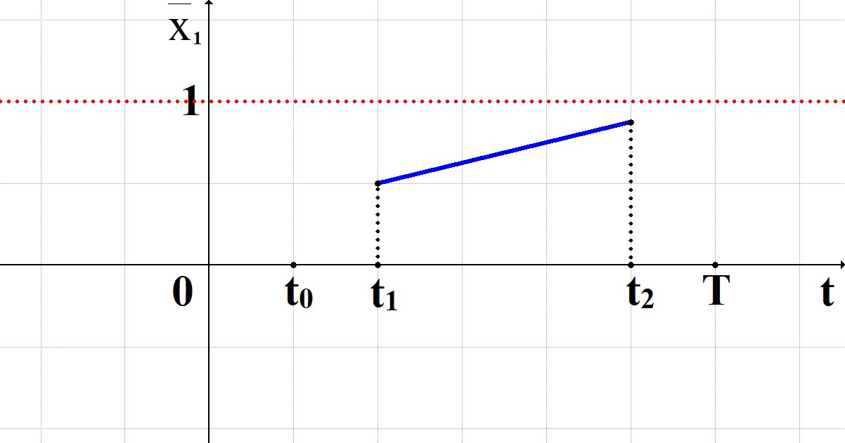 Figure 1
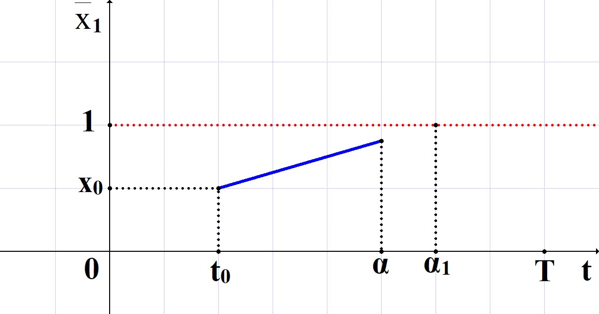 Figure 2
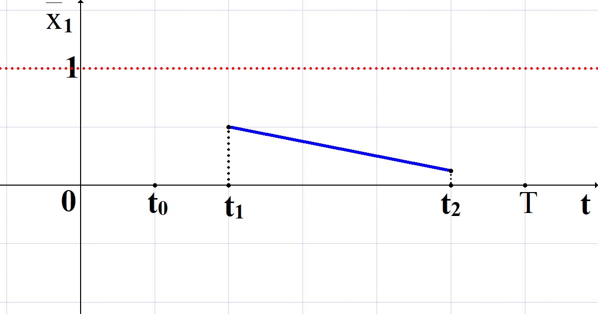 Figure 3
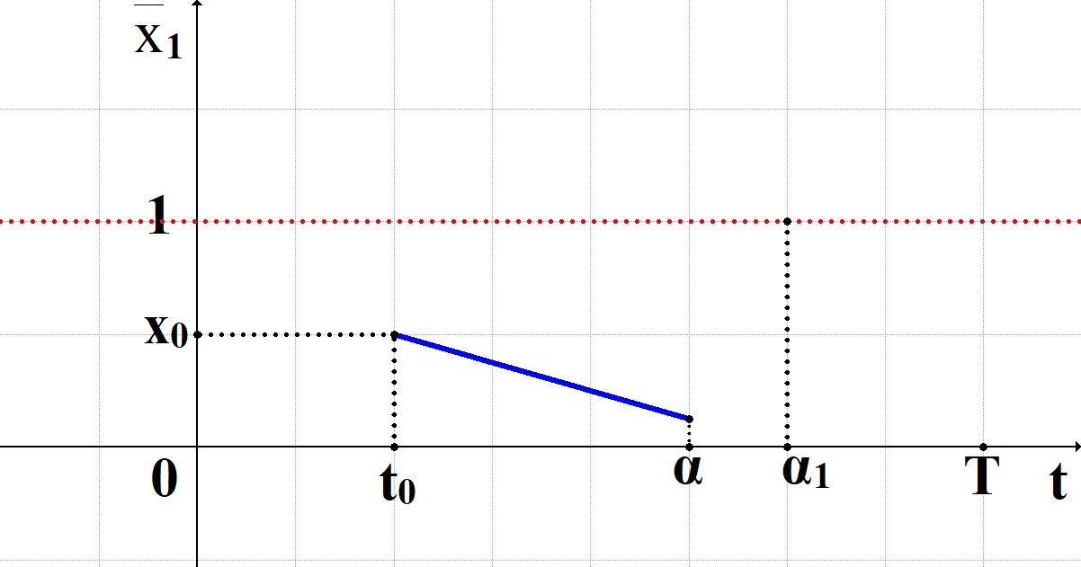 Figure 4
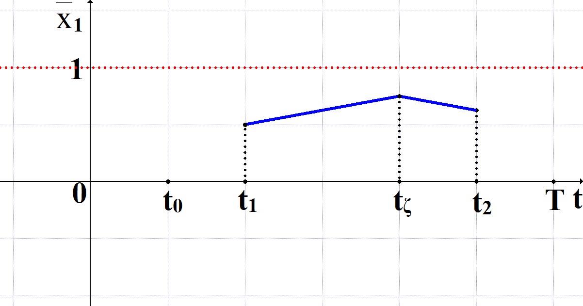 Figure 5
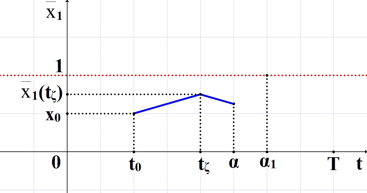 Figure 6