Localizing the $E_2$ page of the Adams spectral sequence
Eva Belmont

TL;DR
This paper investigates the localized structure of the Adams spectral sequence at prime 3, computing differentials up to the E9 page and conjecturing collapse, revealing new insights into the algebraic topology of spheres.
Contribution
It provides the first detailed computation of the localized Adams E2 page at prime 3, including differential analysis and conjectured spectral sequence collapse.
Findings
Computed up to E9 page of the spectral sequence
Conjectured spectral sequence collapses at E9
Complete calculation of localized Ext groups
Abstract
There is only one nontrivial localization of (the chromatic localization at ), but there are infinitely many nontrivial localizations of the Adams page for the sphere. The first non-nilpotent element in the page after is . We work at and study (where is the algebra of dual reduced powers), which agrees with the infinite summand of above a line of slope . We compute up to the page of an Adams spectral sequence in the category converging to , and conjecture that the spectral sequence collapses at . We also give a complete calculation of…
Click any figure to enlarge with its caption.
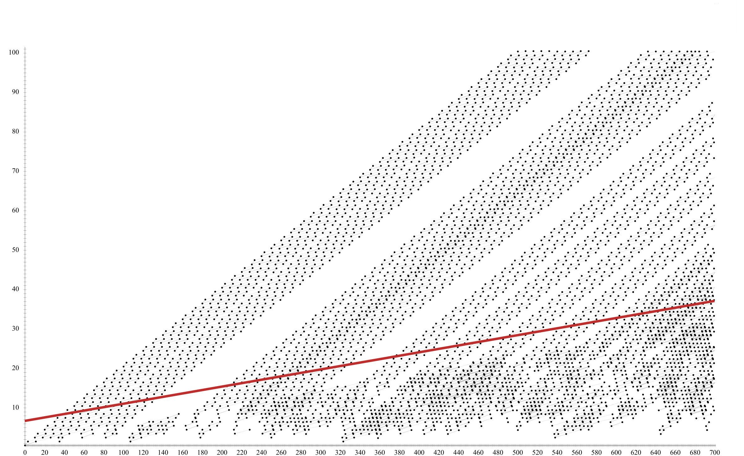 Figure 1
 Figure 2
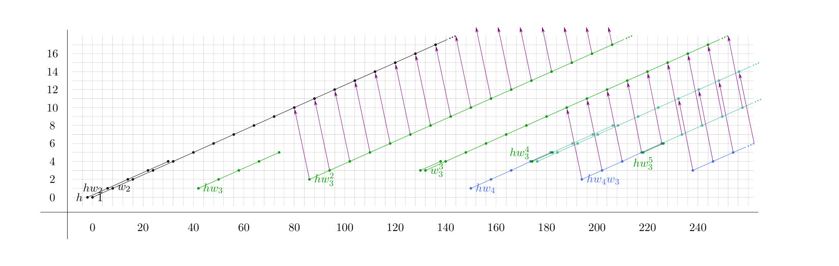 Figure 3
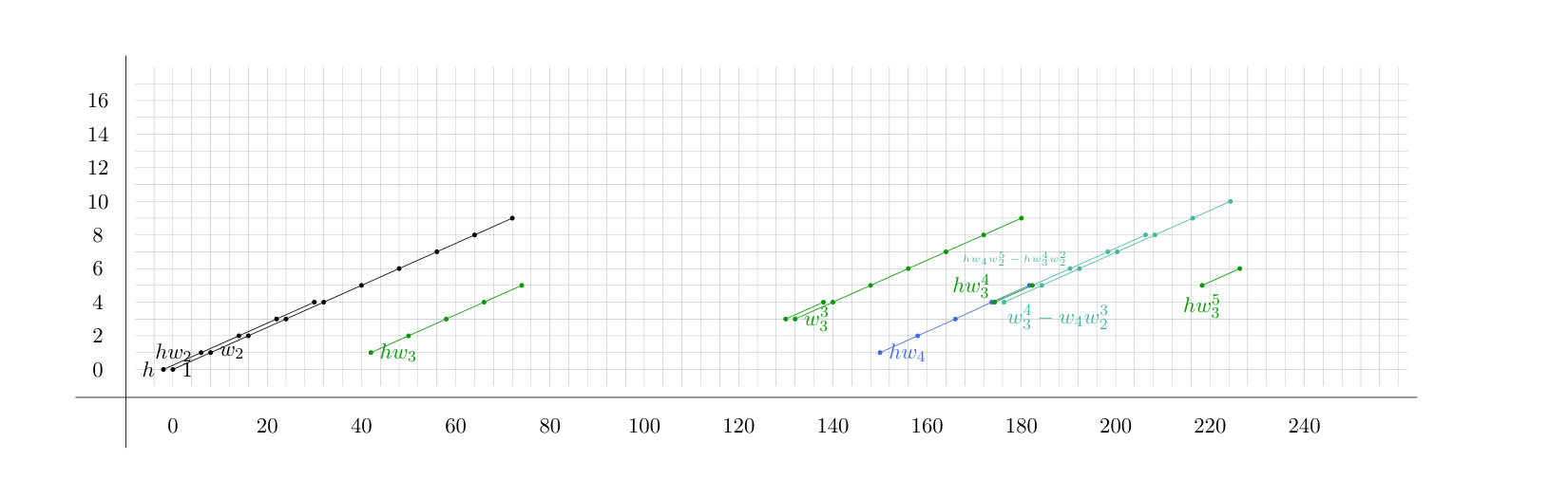 Figure 4
| element | |||||
| 1 | 1 | 4 | 0 | ||
| 3 | 2 | 12 | 0 | 0 | |
| 3 | 1 | 12 | 6 | 0 | |
| 9 | 2 | 36 | 24 | 0 | |
| 1 | 1 | 16 | 10 | 0 | |
| 3 | 2 | 48 | 36 | 0 | |
| 1 | 1 | 0 | |||
| 3 | 2 | 0 | |||
| 3 | 1 | 3 | |||
| 9 | 2 | 9 | |||
| 9 | 1 | 9 | |||
| 27 | 2 | 27 | |||
| 1 | 1 | 3 | |||
| 3 | 2 | 9 | |||
| 3 | 1 | 9 | |||
| 9 | 2 | 27 | |||
| 1 | 1 | 9 | |||
| 3 | 2 | 27 |
Peer Reviews
No public reviews on file for this paper yet. If you reviewed it on a platform where reviews are public (OpenReview, ICLR, NeurIPS, ICML), you can paste yours below so the community can read it here.
Videos
No videos yet. Explain this paper in a talk, walkthrough, or lecture? Add one.
Localizing the page of the Adams spectral sequence
Eva Belmont
Abstract.
There is only one nontrivial localization of (the chromatic localization at ), but there are infinitely many nontrivial localizations of the Adams page for the sphere. The first non-nilpotent element in the page after is . We work at and study (where is the algebra of dual reduced powers), which agrees with the infinite summand of above a line of slope . We compute up to the page of an Adams spectral sequence in the category converging to , and conjecture that the spectral sequence collapses at . We also give a complete calculation of .
Contents
- 1 Introduction
- 2 Overview of the MPASS converging to
- 3 Identifying the -periodic region
- 4 -module structure of at
- 5 Hopf algebra structure of at
- 6 Computation of
- 7 Some results on higher differentials
- 8 Localized cohomology of a large quotient of
1. Introduction
For a -local finite spectrum , the Adams spectral sequence
[TABLE]
is one of the main tools for computing (the -completion of) the homotopy groups of . If one understands the -comodule structure of , it is possible to compute the page algorithmically in a finite range of dimensions. However, for many spectra of interest such as the sphere spectrum, there is no chance of determining the page completely. The motivating goal behind this work is to compute an infinite part of the Adams page for the sphere at . Specifically, we wish to compute the -periodic part, where converges to . We show that there is a plane above which is -periodic, where the third grading (in addition to internal degree and homological degree ) is related to the collapse of the Cartan-Eilenberg spectral sequence at odd primes (see (1.2)).
The only known localization of the Adams page for the sphere is
[TABLE]
where converges to ; this follows from Adams’ fundamental work [Ada66] on the structure of the page. This localization agrees with above a line of slope (in the grading). Our proposed localization agrees with above a plane whose fixed- cross section is a line of slope . While the only -periodic elements lie in the zero-stem (corresponding to chromatic height zero), the -periodic region encompasses nonzero classes in arbitrarily high stems, including some elements in chromatic height 2, such as itself. Though we do not give a complete calculation of , we will see that it is much more complicated than . Thus in some sense, one may think of as a richer and more revealing version of the classical calculation.
In a different sense, however, these two localizations come from different worlds. Inverting is the Adams avatar of -localization on (-local) homotopy (rationalization). Equivalently, the sphere has chromatic type zero, and is just the algebraic name for the chromatic height-0 operator . On the other hand, inverting is not the shadow of any homotopy-theoretic localization: by the Nishida nilpotence theorem, is nilpotent in homotopy, so . While is the only chromatic periodicity operator acting on the sphere, and are just the first two out of infinitely many non-nilpotent elements in . Palmieri [Pal01] describes a more complicated analogue of the classical theory of periodicity and nilpotence that operates only on Adams pages, almost all of which (except the operators) is destroyed by the time one reaches the Adams page.
Recall that the odd-primary dual Steenrod algebra has a presentation where denotes an exterior algebra, and . Let be the Steenrod reduced powers algebra, and let be the quotient Hopf algebra . If is an evenly graded -comodule, there is an isomorphism
[TABLE]
which arises from the collapse of the Cartan-Eilenberg spectral sequence at odd primes . In light of this, we recast our goal as follows:
Goal 1.1**.**
Compute for -comodules .
In particular, we are most interested in . In this paper, we focus on the summand . We show:
Theorem 1.2**.**
Let and let . There is a spectral sequence
[TABLE]
where has filtration 1, internal homological degree 1, and internal topological degree . For degree reasons, for unless or . The first nontrivial differential is
[TABLE]
Furthermore, we give a complete description of the ’s.
We conjecture that the spectral sequence collapses at , and show that this is equivalent to the following conjecture.
Conjecture 1.3**.**
There is an isomorphism
[TABLE]
where with and coaction given by for . (These generators are related to the generators of Theorem 1.2 by .)
Adams’ theorem (1.1) has the more general form
[TABLE]
for an -comodule (see also [MM81]). In particular, the localized cohomology depends only on the -comodule structure on . The analogous statement for -localization (that depends only on the -comodule structure of ) is not true. In general, we propose the following:
Conjecture 1.4**.**
There is a functor such that
[TABLE]
and, as vector spaces, agrees with the page of the spectral sequence described below in Theorem 1.6 with .
Our best complete result is the following; it is proved in Section 8 using different methods.
Theorem 1.5**.**
There is an isomorphism
[TABLE]
where acts trivially on all the generators on the right.
1.1. Main tool
Our main tool (the spectral sequence mentioned in Theorem 1.2) is as follows. It is a special case of the construction discussed in [Bel18].
Theorem 1.6**.**
Let and let be a Hopf algebra over with a surjection of Hopf algebras . Let B_{\Gamma}=\Gamma\,\text{\square}_{D}\mathbb{F}_{p}. For a -comodule , there is a spectral sequence
[TABLE]
(where is the coaugmentation ideal ). At , is flat as a -module, and
[TABLE]
We work at throughout. The main focus is the case and B_{P}=P\,\text{\square}_{D}\mathbb{F}_{3}\equalscolon B; this is the spectral sequence of Theorem 1.2. We also apply this for two quotients of —for a spectral sequence comparison argument in Section 6 and for the proof of Theorem 1.5 in Section 8. Convergence is proved in Appendix A in the case that is a quotient of .
In [Bel18], we show that the following three constructions of (1.3) coincide at the page.
- (1)
The first construction is a -localized Cartan-Eilenberg-type spectral sequence associated to the sequence of -comodule algebras . (Note that the inclusion is not a map of coalgebras; see [Bel18, §2.3] for a precise construction in this case.) 2. (2)
The second construction is an Adams spectral sequence internal to the category . See [Mar83, Chapter 14] or [HPS97, §9.6] for a definition of for a Hopf algebra over , or [BHV15, §4] for a more modern viewpoint; the idea is that it is a variation of the derived category of -comodules designed to satisfy . In particular, if is a -comodule, then . The Adams spectral sequence in this setting was first studied by Margolis [Mar83] and Palmieri [Pal01], and so we call this the Margolis-Palmieri Adams spectral sequence (MPASS).
In particular, let (where the colimit is taken in ); then our spectral sequence is the -based Adams spectral sequence. 3. (3)
The third construction is obtained by -localizing the filtration spectral sequence on the normalized -cobar complex in which if at least of the ’s lie in .
Our dominant viewpoint will be via the framework of (2), but the other two formulations will be useful at key moments. By a “-localized” spectral sequence, we mean the spectral sequence whose page is obtained by -localizing the original page. It is not automatic that this converges to the -localization of the original spectral sequence; this is what is checked in Appendix A.
The essential reason we focus on is that for the analogous construction at , the flatness condition does not hold. (This comes from the Adams spectral sequence flatness condition applied in the setting of (2).)
1.2. Outline
In Section 2, we prove some basic results about the structure of the spectral sequence converging to and introduce definitions and notation that will be used extensively in the computational sections. In Section 3, we apply vanishing line results to describe a region in which agrees with . Sections 4 and 5 are devoted to computing the page of the -based MPASS converging to . In Section 6 we determine , the first nontrivial differential after the page. In Section 7, we determine and show that our conjecture that the spectral sequence collapses at would imply the desired form of in Conjecture 1.3. In Section 8 we prove Theorem 1.5. In Appendix A we show convergence of the MPASS in the cases of interest, and also show convergence of an auxiliary spectral sequence needed for Section 6.
1.3. Acknowledgements
I am grateful to Haynes Miller, my graduate advisor, for suggesting this as a thesis project and for providing invaluable guidance at every step along the way. I would also like to thank Dan Isaksen and Zhouli Xu for helpful conversations about this work, and Hood Chatham for productive conversations and for the spectral sequences LaTeX package used to draw the charts in Appendix B.
2. Overview of the MPASS converging to
In every section except Sections 3 and 4 we will set and let . We will denote exterior and truncated polynomial algebras, respectively, by and . Let .
If is a -comodule and , we adopt the notation of [Pal01] and write:
[TABLE]
Here is given the diagonal -comodule structure: where and . Define
[TABLE]
where the colimit is taken in . Due to the general machinery of Adams spectral sequences in (see [Pal01, §1.4]), we have a -based spectral sequence
[TABLE]
which we call the -based Margolis-Palmieri Adams spectral sequence (MPASS). Here denotes coaugmentation ideal. By the shear isomorphism (Lemma 5.16) and the change of rings theorem, we may write . If is flat over , then the page (2.1) has the form
[TABLE]
The differential is a map . Here is the MPASS filtration, is the internal homological degree, and is the internal topological degree. Furthermore, we will often find it convenient to work with the degree
[TABLE]
which has the property that . In this grading, the differential is a map .
The coefficient ring is easy to compute using the change of rings theorem:
[TABLE]
where is in homological degree 1 and is in homological degree 2. It will be useful to have notation for this coefficient ring:
[TABLE]
Using the shear isomorphism (Lemma 5.16) and the change of rings theorem, we have
[TABLE]
Notation 2.1**.**
We have chosen to define as a left -comodule. It can be written explicitly as . To simplify the notation, from now on we will redefine the symbol to mean the antipode of the usual . Thus, going forward, we will have , and
[TABLE]
In Section 5, we will show that the flatness condition holds and is isomorphic, as a Hopf algebra over , to an exterior algebra on generators
[TABLE]
This implies that the page is isomorphic to a polynomial algebra over on classes of degree .
The generator is a permanent cycle, and converges to . We will see in Section 6 that the other ’s support differentials, so it is less easy to see how these generators connect to familiar elements in the Adams page. One heuristic comes from looking at the images of these classes in : in that setting, and .
Let and . Then , and using simple degree arguments, we will show that higher differentials take to and vice versa.
Lemma 2.2**.**
Suppose is nonzero. If , then and . Otherwise, , in which case and .
Proof.
This can be read off the following table of degrees.
[TABLE]
∎
Proposition 2.3**.**
If and or , then . Furthermore,
[TABLE]
Proof.
This is a degree argument, so we simplify to considering where is a monomial. First notice that . If , then is even; if , then is odd. Thus and .
If , then . If , Lemma 2.2 implies and , so . Similarly, if , then , which implies if . ∎
In Section 7, we show that if is the first nontrivial differential on , and , then . Combined with our complete calculation of in Section 6, this determines the spectral sequence through the page. We conjecture that the spectral sequence collapses at . The idea is that there is an operator defined by where for , and that the spectral sequence essentially operates by taking Margolis homology of this operator: if supports a nontrivial , then , and .
Remark 2.4**.**
It is tempting to expect that Conjecture 1.3 comes from a map k\to P\,\text{\square}_{D}\widetilde{W}, which would induce a map b_{10}^{-1}\operatorname{Ext}_{P}^{*}(k,k)\to b_{10}^{-1}\operatorname{Ext}_{P}^{*}(k,P\,\text{\square}_{D}\widetilde{W})\cong b_{10}^{-1}\operatorname{Ext}_{D}^{*}(k,\widetilde{W}) by the change of rings theorem. However, this is not the case: k\to P\,\text{\square}_{D}\widetilde{W} would factor through P\,\text{\square}_{D}k, which would mean that the map in would factor through b_{10}^{-1}\operatorname{Ext}_{P}^{*}(k,P\,\text{\square}_{D}k)\cong R.
3. Identifying the -periodic region
In this section, let be an odd prime and let . The following characterization of a -periodic region in Ext is a consequence of results of Palmieri that generalize the vanishing line theorems of Miller and Wilkerson [MW81] to the stable category of comodules.
Proposition 3.1**.**
The localization map is an isomorphism in the range for some constant .
Our main input is the following theorem, which Palmieri states for the Steenrod dual instead of the algebra of dual reduced powers, as we do below. The necessary changes in the case of follow immediately from the discussion in [Pal01, §2.3.2].111The only difference is that, over , one must also take into account the objects corresponding to ’s as opposed to ’s, which do not come into play over .
Following Palmieri [Pal01, Notation 2.2.8], define the slope of to be:
[TABLE]
Let denote the truncated polynomial algebra . We have . Let K(\xi_{t}^{p^{s}})=b_{ts}^{-1}(P\,\text{\square}_{D[\xi_{t}^{p^{s}}]}k), where the localization is defined by taking a colimit of multiplication by in .
Theorem 3.2** ([Pal01, Theorem 2.3.1]).**
Suppose is an object in satisfying the following conditions:
- (1)
There exists an integer such that if , 2. (2)
There exists an integer such that if , 3. (3)
There exists an integer such that the homology of the cochain complex vanishes in homological degree . (In particular, this is satisfied if is the resolution of a bounded-below comodule.)
Suppose (with ) has the property that for all with and . Then has a vanishing line of slope : for some , when .
Proof of Proposition 3.1.
Let denote the cofiber in of , thought of as a map in . It is not hard to check the conditions (1)–(3) of Theorem 3.2 for . We will apply the theorem with ; note that is the next with and higher slope than , so we just have to check . This follows because the cofiber sequence
[TABLE]
gives rise to a long exact sequence in , and multiplication by is an isomorphism on by construction. So the theorem implies that there exists some such that when .
Applying to (3.1), we obtain
[TABLE]
where . Applying the vanishing condition for directly gives a region in which multiplication by is an isomorphism. ∎
In particular, at , agrees with above a line of slope (see Figure 1). In [Pal01, 2.3.5(c)], Palmieri gives an explicit expression for the constant, which allows us to calculate the -intercept to be .
4. -module structure of at
In this section, we work at an arbitrary odd prime, and let and .
In preparation for studying the page , our goal for the next two sections is to study the Hopf algebra , which in (2.3) we showed is isomorphic to . Most of this section is devoted to giving an expression for as a -comodule. In the next section, we will obtain a more explicit description at , in which case we calculate the page.
4.1. -comodule structure of
Note that is an algebra and a -comodule, but not a coalgebra. Let denote the -coaction that comes from composing the -coaction with the surjection .
Definition 4.1**.**
If we write
[TABLE]
for some ’s, define
[TABLE]
For example, since (using the convention of Notation 2.1), we have , and . One can show using coassociativity that . As is dual to in the Steenrod algebra, the operator is dual to the operator given by left -multiplication. In particular, implies .
Lemma 4.2**.**
* is the cohomology of the chain complex , and is the cohomology of the unbounded chain complex .*
Lemma 4.3**.**
We have .
Proof.
We have
[TABLE]
The structure theorem for modules over a PID says that modules over decompose as sums of modules isomorphic to for . Dually, we have the following:
Lemma 4.4**.**
Let denote the -comodule . Then every -comodule splits uniquely as a direct sum of -comodules isomorphic to for .
Note that and .
Remark 4.5**.**
Since is a 1-dimensional vector space in homological degree 0 and zero otherwise, for any free -comodule . If , is 1-dimensional in every homological degree.
The goal is to prove the following proposition.
Proposition 4.6**.**
Define the indexing set to be the set of monomials of the form such that , and for , write and . Then there is a -comodule isomorphism
[TABLE]
where is a free -comodule, the tensor product is endowed with the diagonal -comodule structure, and .
Corollary 4.7**.**
We have an -module isomorphism
[TABLE]
Remark 4.8**.**
There is a formula due to Renaud [Ren79, Theorem 1] that allows one to decompose the tensor products into a sum of the basic comodules , but in general it is rather complicated; instead we will do this in the next section only at .
If then is a sub--comodule of with dimension . By the Leibniz rule (Lemma 4.3) we have
[TABLE]
for . For any collection of , define
[TABLE]
This is a sub--comodule spanned (as a vector space) by monomials of the form . Clearly, , but this is not a direct sum decomposition—any given monomial appears in many different summands. To fix this, we will study the poset of ’s, and find that is a direct sum of the maximal elements of that poset.
Notation 4.9**.**
Define the notation
[TABLE]
(These are not formal products; they only make sense if for all but finitely many .) For example, we have for any monomial , and . Expressions represent elements of , and conversely every element of has a representation of this form (note that ). Monomials in do not have unique expressions of the form : for example, .
Lemma 4.10**.**
There is a bijection
[TABLE]
Say that a bracket expression is admissible if it is of the form on the right hand side.
Proof.
Given a monomial, the admissible bracket expression is the one with the greatest number of terms on the right-hand side. ∎
Lemma 4.11**.**
If is a monomial with admissible bracket expression and is a monomial in , then (up to invertible scalar) has admissible expression for a set of that are zero for all but finitely many .
The idea is that is obtained from by moving terms from the left to the right.
Proof.
If then we have
[TABLE]
By definition, where , and
[TABLE]
using the fact that . So we can take in the lemma statement. ∎
Definition 4.12**.**
For monomials and , write if .
It is easy to check that this makes the set of monomials into a poset, and that if and only if .
Lemma 4.13**.**
Suppose is a monomial with admissible bracket expression . Let where and . Then is the maximal object .
Proof.
Let be an arbitrary monomial, written in its unique admissible bracket expression. Then if and only can be obtained from by moving terms in from the right to the left side of the bracket expression. Note that is the bracket expression obtained by moving as many terms to the left as possible while still keeping the resulting expression admissible. This implies is maximal. ∎
Define an equivalence relation on monomials where if .
Lemma 4.14**.**
There is a direct sum decomposition .
Proof.
I claim that ; this follows from the fact that, by definition, is generated by such that . So the direct sum decomposition comes from partitioning monomials into their equivalence classes. ∎
Let be the set of admissible bracket expressions such that . By Lemma 4.13 we have the following.
Lemma 4.15**.**
* is the set of admissible bracket expressions such that and if then .*
Lemma 4.16**.**
If is an admissible expression, there is an isomorphism of -comodules .
Proof.
By Lemma 4.11, every in has a bracket expression obtained from by moving terms from the left to the right, so the right hand side of the bracket expression for is divisible by , and so is divisible by . So multiplication by gives a map , and moreover from the above description of it is easy to see that this is a bijection. Finally, since , this is an isomorphism of -comodules. ∎
Lemma 4.17**.**
If is an admissible expression such that for some then is a free -comodule.
Proof.
By definition, we have where the tensor product is endowed with the diagonal -comodule structure and by assumption. After rearranging terms, it suffices to show that, for any -comodule , there is a -comodule isomorphism where the left hand side has a diagonal -coaction and the right hand side has a left coaction ( vs. where and ). This isomorphism is a variant of the shear isomorphism of Lemma 5.16, and is given by . ∎
By Lemmas 4.16 and 4.17, we have:
Corollary 4.18**.**
If is an admissible bracket expression in such that for any , then is free as a -comodule.
Proof of Proposition 4.6.
From Lemma 4.14 we have , and by Corollary 4.18 there are free -comodules and such that
[TABLE]
We conclude this section with a useful lemma that simplifies checking relations in certain -local Ext groups of interest.
Lemma 4.19**.**
Let . Then is contained in the free part of according to the decomposition in Proposition 4.6. In particular, if x\in\operatorname{Ext}^{*}_{P}(k,P\,\text{\square}_{D}I(p-1)) then in b_{10}^{-1}\operatorname{Ext}^{*}_{P}(k,P\,\text{\square}_{D}B).
Proof.
Consider an arbitrary monomial in . If has an admissible expression then has an admissible expression . By Lemmas 4.14 and 4.17, it suffices to show that satisfies for some . Using the formula for in Lemma 4.13, we have . ∎
Corollary 4.20**.**
Let be as in Lemma 4.19. If x\in\operatorname{Ext}_{P}^{*}(k,P\,\text{\square}_{D}(P\,\text{\square}_{D}I(p-1))), then is zero in b_{10}^{-1}\operatorname{Ext}_{P}^{*}(k,P\,\text{\square}_{D}(P\,\text{\square}_{D}I(p-1))).
5. Hopf algebra structure of at
Henceforth we will work at . This assumption will allow us to simplify the formula for obtained in Corollary 4.7 and show that is flat over (this is not true at higher primes), enabling us to calculate the page (2.1) of the -based MPASS. In particular, our goal is to show the following:
Theorem 5.1**.**
At , the ring of co-operations is flat over , and moreover there is an isomorphism of Hopf algebras
[TABLE]
for generators in internal topological degree . That is, is primitive, and is exterior as a Hopf algebra over .
Plugging this into the expression (2.1) for the page, we obtain:
Corollary 5.2**.**
The page of the -based MPASS for computing is
[TABLE]
where .
Remark 5.3**.**
As is a -comodule algebra, there is a Hopf algebroid in , where carries the diagonal coaction of (see Section 2) and the comultiplication is given by
[TABLE]
The Hopf algebroid above is given by applying to this one.
5.1. Vector space structure of at
In the case, Corollary 4.7 reads
[TABLE]
where the tensor product has a diagonal -coaction. It is easy to see directly that . (Here we use bigraded notation for the shift for consistency with viewing these objects in , so denotes a shift of 0 in the homological dimension and in internal degree). In particular,
[TABLE]
After inverting , free comodules become zero, and the only basic types of comodules are and .
Lemma 5.4**.**
In , we have an isomorphism
[TABLE]
Proof.
A representative for in (i.e., an injective resolution for it) is , and so is represented by
[TABLE]
Similarly, is represented by
[TABLE]
and so there is a degree-preserving isomorphism . ∎
(At arbitrary primes, the formula holds for the same reason.) Therefore, if is a -comodule, then is a sum of shifts of the unit object . Remembering that was constructed so that , we obtain the following Künneth isomorphism:
Lemma 5.5** (Künneth isomorphism for ).**
If and are -comodules, then
[TABLE]
This only works at , and is the essential reason we have made the simplification of working at .
Applying this to (4.1) we have the following.
Corollary 5.6**.**
We have an isomorphism
[TABLE]
where is the copy of isomorphic to under Lemma 5.4. In particular, is free over .
So has -module generators in bijection with monomials of the form (where if ). Now we will be more precise in choosing these generators.
Lemma 5.7**.**
Suppose is a -comodule algebra with sub--comodules and .
- (1)
The image of in is generated by
[TABLE] 2. (2)
We have
[TABLE]
in the multiplication induced by the product structure on . In particular, . 3. (3)
If the multiplication map embeds in injectively, then is a 1-dimensional vector space with generator .
Since for , note that this also gives a generator of .
Proof.
Since is a 1-dimensional -vector space, for (1) it suffices to show that is a cycle that is not a boundary. Indeed, since and , we have , and is not in .
For (2), we use a special case of the cobar complex multiplication formula in [Mil78, Proposition 1.2]:
Fact 5.8**.**
The multiplication is given by
[TABLE]
Thus the product takes . Using this formula, we have:
[TABLE]
For (3), note that there is a decomposition of -comodules
[TABLE]
and since , the quotient map
[TABLE]
is an isomorphism. By (2), is a generator of the latter Ext group. ∎
Lemma 5.9**.**
Suppose is a -comodule algebra with sub--comodules and .
- (1)
The image of in is generated by . 2. (2)
We have
[TABLE] 3. (3)
If the multiplication map embeds in injectively, then is a generator of the 1-dimensional vector space .
Proof.
(1) is clear. (2) follows from the cobar complex multiplication formulas
[TABLE]
For (3), note that . Note that . From Lemma 5.7, is generated by . ∎
Definition 5.10**.**
Define as the chosen generator of .
Lemma 5.11**.**
Under the change of rings isomorphism
[TABLE]
the image of in \operatorname{Ext}^{1}_{P}(k,P\,\text{\square}_{D}B) has cobar representative
[TABLE]
Proof.
The change of rings isomorphism \operatorname{Ext}_{D}(k,M)\cong\operatorname{Ext}_{P}(k,P\,\text{\square}_{D}M) works as follows: since is free over , the functor P\,\text{\square}_{D}- is exact, and so given an injective -resolution for , the complex P\,\text{\square}_{D}M\to P\,\text{\square}_{D}X^{\bullet} is an injective -resolution. So we have \operatorname{Ext}^{i}_{D}(k,M)\cong\operatorname{Cotor}^{i}_{D}(k,M)=H^{i}(k\,\text{\square}_{D}X^{\bullet}), which agrees with \operatorname{Ext}^{i}_{P}(k,P\,\text{\square}_{D}M)\cong\operatorname{Cotor}^{i}_{P}(k,P\,\text{\square}_{D}M)=H^{i}(k\,\text{\square}_{P}(P\,\text{\square}_{D}X^{\bullet}))\cong H^{i}(k\,\text{\square}_{D}X^{\bullet}).
In particular, \operatorname{Ext}_{P}(k,P\,\text{\square}_{D}B) can be computed by applying k\,\text{\square}_{P}- to the resolution
[TABLE]
By Lemma 5.7, has representative in the -cobar resolution for , and so its representative in (5.1) is .
But we wanted a representative in the cobar complex C_{P}(k,P\,\text{\square}_{D}B), so we will write down part of an explicit map from the -cobar resolution for P\,\text{\square}_{D}B to (5.1):
[TABLE]
By basic homological algebra, the map exists and is unique, so to find and it suffices to find -comodule maps that make the first two squares commute. In particular, one can check that the maps
[TABLE]
make the diagram commute, and is a cycle in P\otimes{\overline{P}}\otimes(P\,\text{\square}_{D}B) such that (k\,\text{\square}_{P}f)(z)=e(x). ∎
5.2. Multiplicative structure
Proposition 5.12**.**
The summand
[TABLE]
is generated by the product .
Proof.
Since
[TABLE]
it suffices to show that is generated by when is even, and is generated by when is odd. We proceed by induction on . The base case is by definition.
Case 1: is even. The tensor product is isomorphic to for a free summand . By Lemma 5.7, is generated by where is a generator of . By the inductive hypothesis, we can take . So then is a generator for .
Case 2: is odd. In this case, is isomorphic to for a free summand . By Lemma 5.9, is generated by where is a generator of . By the inductive hypothesis, we can take . ∎
Recall we defined .
Corollary 5.13**.**
There is an -module isomorphism where the generator is in degree .
Corollary 5.14**.**
The map is an isomorphism of -algebras.
5.3. Antipode
The antipode is the map induced on by the swap map . In order to get a useful formula for this map, we will need the following basic properties of Hopf algebras.
Fact 5.15**.**
Denote the coproduct on an element of a Hopf algebra by .
- (1)
(coassociativity) 2. (2)
** 3. (3)
** 4. (4)
**
Lemma 5.16** (Shear isomorphism).**
Suppose is a left -comodule, and is given the diagonal -coaction: (where and ). Then there is an isomorphism S_{M}:B\otimes M\to P\,\text{\square}_{D}M (where coacts on the left on P\,\text{\square}_{D}M) sending . It has an inverse .
In order to be able to apply Lemma 4.19, we now obtain an explicit formula for the induced map \tau^{\prime}\colonequals S_{B}\circ\tau\circ S_{B}^{-1}:P\,\text{\square}_{D}B\to P\,\text{\square}_{D}B. This map is:
[TABLE]
Using Fact 5.15 we have:
[TABLE]
Since is a Hopf algebroid, the antipode is multiplicative, so to determine it, it suffices to show:
Proposition 5.17**.**
We have:
- (1)
** 2. (2)
.
Proof.
The antipode is given by the map \tau^{\prime}_{*}:\operatorname{Ext}_{P}^{*}(k,P\,\text{\square}_{D}B)\to\operatorname{Ext}_{P}^{*}(k,P\,\text{\square}_{D}B) induced by , defined so that . Since h=[\xi_{1}](1|1)\in\operatorname{Ext}^{1}_{P}(k,P\,\text{\square}_{D}B), we have . For (2), we need an explicit formula for the antipode in the dual Steenrod algebra:
Fact 5.18** ([Mil58, Lemma 10]).**
Let be the set of ordered partitions of , the length of the partition , and be the partial sum. Then we have:
[TABLE]
In particular, if then and .
Recall (Notation 2.1) that we have defined to be the antipode of its usual definition, so here we have . (Since the antipode is a ring homomorphism, the formula in Fact 5.18 is the same in either case.)
Combining this antipode formula with the formula for in Lemma 5.11 we have:
[TABLE]
for , , , and in . By Lemma 4.19 these terms are zero in -local cohomology, and . ∎
Corollary 5.19**.**
We have ; that is, the Hopf algebroid is, in fact, a Hopf algebra.
Proof.
One of the axioms of a Hopf algebroid is . Since is just the inclusion of into , its image is invariant under the antipode . ∎
5.4. Comultiplication
To define the comultiplication map
[TABLE]
first consider the maps
[TABLE]
where is the map on Ext induced by with , and is defined as the map in the factorization
[TABLE]
It follows from the shear isomorphism (Lemma 5.16) and the change of rings theorem that \operatorname{Ext}_{P}(k,B\otimes M)\cong\operatorname{Ext}_{P}(k,P\,\text{\square}_{D}M)\cong\operatorname{Ext}_{D}(k,M), and the Künneth isomorphism for -local cohomology over (Lemma 5.5) implies that is an isomorphism after inverting . We define the comultiplication map on by .
In particular, flatness of over implies that is a Hopf algebroid using the definitions of comultiplication, antipode, counit, and unit above. In a Hopf algebroid, the comultiplication is a homomorphism, and so to determine explicitly it suffices to determine . We prove this in Proposition 5.21. Lemma 5.11 gives an expression for in \operatorname{Ext}_{P}^{1}(k,P\,\text{\square}_{D}B), so we prefer to calculate after composing with the shear isomorphism; that is, there is a commutative diagram
[TABLE]
and we will show that in b_{10}^{-1}\operatorname{Ext}_{P}(k,P\,\text{\square}_{D}(P\,\text{\square}_{D}B)). (We have chosen to use an extra application of the shear isomorphism on the middle term in order to apply Corollary 4.20.)
Lemma 5.20**.**
If a\in\operatorname{Ext}_{P}(k,P\,\text{\square}_{D}B) has cobar representative , we have
[TABLE]
in \operatorname{Ext}_{P}(k,P\,\text{\square}_{D}(P\,\text{\square}_{D}B)).
So to check that is primitive after inverting , it suffices to check
[TABLE]
in b_{10}^{-1}\operatorname{Ext}_{P}(k,P\,\text{\square}_{D}(P\,\text{\square}_{D}B)).
Proof.
By definition, is the map induced on by the composition
[TABLE]
On elements, we have:
[TABLE]
where the last equality is a coassociativity argument similar to the one at the beginning of Section 5.3. That is, we have , which implies
[TABLE]
The map comes from the bottom composition in
[TABLE]
We will only give an explicit expression for on elements of the form and , where denotes the unit 1\otimes 1\in\operatorname{Ext}_{P}^{0}(k,P\,\text{\square}_{D}B) and a=[a_{1}|\dots|a_{s}](p\otimes q)\in\operatorname{Ext}_{P}^{s}(k,P\,\text{\square}_{D}B). In [Mil78], there is a full description of the Künneth map on the level of cochains, but here all we need are the maps and . The former sends and the latter sends . In particular, and in \operatorname{Ext}_{P}^{s}(k,(P\,\text{\square}_{D}B)\otimes(P\,\text{\square}_{D}B)).
To determine , it remains to determine the map \gamma:(P\,\text{\square}_{D}B)\otimes(P\,\text{\square}_{D}B)\to P\,\text{\square}_{D}(P\,\text{\square}_{D}B) induced by . This is accomplished by calculating the effect of shear isomorphisms as follows:
[TABLE]
[TABLE]
That is, , which implies
[TABLE]
Proposition 5.21**.**
The element is primitive.
Proof.
We need to check the criterion (5.3) for . Recall we had the formula
[TABLE]
from Lemma 5.11. It suffices to check that is zero in b_{10}^{-1}\operatorname{Ext}_{P}(k,P\,\text{\square}_{D}(P\,\text{\square}_{D}B)). Using Lemma 5.20 we have:
[TABLE]
But all the remaining terms in the difference are in C_{P}(P\,\text{\square}_{D}(P\,\text{\square}_{D}I(3))) so by Corollary 4.20 they are zero in -local cohomology. ∎
Proof of Theorem 5.1.
The flatness assertion was proved in Corollary 5.6. Putting together Lemma 5.14, Proposition 5.17, Corollary 5.19, and Proposition 5.21, we see that the map is an isomorphism of Hopf algebras. ∎
6. Computation of
6.1. Overview of the computation
In the previous section, we’ve shown that the -based MPASS computing has the form
[TABLE]
where is represented in by . Recall that is a map , has degree , has degree , and has degree . Furthermore, , , and . In Proposition 2.3, we have shown that the next nontrivial differential is . In this section we will completely determine this differential. We begin by recording some ’s in low degrees.
Proposition 6.1**.**
We have the following:
[TABLE]
Proof.
The first two facts can be seen directly in the cobar complex , using the cobar representatives and , which are permanent cycles.
The differentials on and were deduced from the chart of up to the 700 stem that appears as Figure 1 (generated by the software [Nas]). In Proposition 3.1, we show that agrees with in the range of dimensions depicted in the chart. Thus we know which classes in in this range of dimensions die in the spectral sequence, and, using multiplicativity of the spectral sequence, this forces the differentials above. ∎
The goal of this section is to prove the following:
Theorem 6.2**.**
For , there is a differential in the MPASS
[TABLE]
Since the spectral sequence is multiplicative, this determines .
The main idea is to use comparison with a spectral sequence computing , where
[TABLE]
(The idea is that this is the smallest algebra in which the desired differential can be seen.) This is a quotient Hopf algebra of by the classification of such (see [Pal01, Theorem 2.1.1.(a)]). Here’s a picture:
\xi_{1}$$\xi_{1}^{3}$$\xi_{2}$$\xi_{n-2}$$\xi_{n-2}^{3}$$\xi_{n-2}^{9}$$\xi_{n-1}$$\xi_{n-1}^{3}$$\xi_{n}
Recall B=P\,\text{\square}_{D}k; let B_{n}=P_{n}\,\text{\square}_{D}k. We will refer to the spectral sequence 1.6 with as the -based MPASS computing , and use to denote its page. For example,
[TABLE]
Let denote the -based MPASS for we have been focusing on. Then the diagram
[TABLE]
shows there is a map of spectral sequences .
Lemma 6.3**.**
It suffices to show that in .
Proof.
Since , we know that is a linear combination of terms of the form . We have
[TABLE]
Note that . Looking at this mod 27, we see that (at least) two of the ’s have to be , say and . Then we have . The only possibility is . So if then , and checking internal degrees shows . ∎
When we discuss it will be easy to see that there is a class which is the target of along the quotient map.
[TABLE]
Lemma 6.3 says that it suffices to show in , but it turns out to be the same amount of work to show the following more attractive statement.
Goal 6.4**.**
There is a differential in .
Using the same argument as Proposition 2.3, we know that in , so is not the target of an earlier differential. We will use the following strategy to show the desired differential in :
- (1)
Calculate in a region and identify classes that are the targets of their namesake classes under the quotient map . 2. (2)
Show that is zero in the stem of . This implies that either supports a differential or is the target of a differential. 3. (3)
Show that is a permanent cycle in the MPASS (so it must be the target of a differential) and show that, for degree reasons, is the only element that can hit it. By looking at filtrations, we see this differential is a .
In order to show (2), we introduce another spectral sequence for calculating , the Ivanovskii spectral sequence (ISS) [Iva64]. This is the (-localized version of the) dual of the May spectral sequence; that is, it is the spectral sequence obtained by filtering the cobar complex on by powers of the augmentation ideal. (For example, has filtration .)
In Section 6.2 we will introduce notation and record facts about gradings. In Section 6.3 we will compute and the relevant part of , and show (1) and (3) assuming (2). In Section 6.4 we will calculate the relevant part of the ISS and show (2). Convergence of the localized ISS is discussed in Section A.2.
6.2. Notation and gradings
Since much of the work in this section consists of degree-counting arguments, we will now record how differentials and convergence affect the various gradings at play. We emphasize a change of coordinates on degrees that simplifies degree arguments by putting in degree zero.
MPASS gradings
In Section 2, we introduced the gradings . The differential has the form
[TABLE]
and a permanent cycle in converges to an element in . We also introduced . We prefer to track instead of , because , so all classes in a -tower have the same -degree. The differential under the change of coordinates has the form
[TABLE]
and a permanent cycle in converges to an element in (where is internal topological degree and is homological degree) with .
Definition 6.5**.**
Let stem in denote the quantity . Then a permanent cycle in converges to an element in the stem.
Finally, define
[TABLE]
This is only useful for looking at the page of the MPASS, as fixes .
ISS gradings
The Ivanovskii spectral sequence computing is the spectral sequence obtained by filtering the cobar complex on by powers of the augmentation ideal. Let denote the page of the Ivanovskii spectral sequence.
We use slightly different grading conventions: classes have degree where is ISS filtration, denotes degree in the cobar complex, and denotes internal topological degree (as in the MPASS). The differential has the form
[TABLE]
and a permanent cycle in converges to an element in .
We will use the change of coordinates
[TABLE]
which is designed so that . (This has a different formula from the MPASS change of coordinates simply because correspond to different parameters here.) The differential has the form
[TABLE]
and a permanent cycle in converges to an element in with , i.e. an element in the stem.
Note that has different formulas for the MPASS and ISS, but in both spectral sequences corresponds to stem, with the definition given above. Now we will introduce another grading on (for ) preserved by the comultiplication.
Extra grading on
Let . Note that every monomial in can be written where and .
Lemma 6.6**.**
For , is a sub-coalgebra of .
Proof.
This is clear from the comultiplication formulas
[TABLE]
and the assumption guarantees that . ∎
Proposition 6.7**.**
Let . There is an extra grading on that respects the comultiplication, defined by the property that it is multiplicative on , and
[TABLE]
Proof.
First we check that respects the comultiplication when restricted to . Since it is defined to be multiplicative on , it suffices to check that for as each of the multiplicative generators. This is clear from the comultiplication formulas (6.2).
Now suppose where . We have
[TABLE]
and the degrees of both sides agree since is a coalgebra. Similarly, if for , we have
[TABLE]
6.3. The page of the -based MPASS
The goal of this section is to prove the following:
Proposition 6.8**.**
If is the target of a differential in the -based MPASS calculating , that differential must be
[TABLE]
The main task is to calculate enough of to do a degree-counting argument (Proposition 6.16), where
[TABLE]
As in the calculation of the page of the -based MPASS (Section 5), the Künneth formula for the functor (Lemma 5.5) guarantees flatness of over . So we can use the formula
[TABLE]
where and by the change of rings theorem. We will simultaneously determine the vector space structure and the comultiplication on .
Remark 6.9**.**
By (6.1) and the Künneth formula mentioned above, we have
[TABLE]
and so the coproduct on coincides with on .
We can write as a tensor product
[TABLE]
illustrated in Figure 2.
Since we have a Künneth formula for , it suffices to apply this functor to each of the four factors of above.
Factor 1: \color[rgb]{0.25390625,0.41015625,0.8828125}\definecolor[named]{pgfstrokecolor}{rgb}{0.25390625,0.41015625,0.8828125}k[\xi_{2},\xi_{1}^{3}]/(\xi_{2}^{3},\xi_{1}^{9})
As a -comodule, this decomposes as:
[TABLE]
(Recall was defined to be the -comodule , and every -comodule is a sum of copies of , , and .) As a module over , this is generated by a class in , a class in , and a class in . As , we may ignore the free summands.
Using Lemma 5.7, we can give explicit representatives for the classes in coming from the decomposition (6.4):
[TABLE]
satisfying relations and .
Lemma 6.10**.**
The classes and are primitive in the coalgebra .
Proof.
As described in Section 1.1, we can interpret the MPASS as a filtration spectral sequence on the cobar complex , where is in filtration if ’s are in . The elements and correspond to elements in with the same formulas, and by Remark 6.9 it suffices to show that in the filtration spectral sequence. One checks explicitly that , so it is a permanent cycle. This is not true of , but we can write down explicit correcting terms in higher filtration:
[TABLE]
and then check that . This has filtration 3, and so . ∎
So we’ve proved:
Proposition 6.11**.**
There is an isomorphism of Hopf algebras
[TABLE]
where and are primitive.
We can summarize the degree information as follows:
[TABLE]
Factor 2: \color[rgb]{0.6953125,0.328125,0.05859375}\definecolor[named]{pgfstrokecolor}{rgb}{0.6953125,0.328125,0.05859375}k[\xi_{n-2}]/\xi_{n-2}^{3}
This decomposes as so we have three -module generators:
[TABLE]
As a Hopf algebra we have
[TABLE]
Factor 3:
\color[rgb]{0,0.58984375,0}\definecolor[named]{pgfstrokecolor}{rgb}{0,0.58984375,0}k[\xi_{n-1},\xi_{n-2}^{3}]/(\xi_{n-1}^{3},\xi_{n-2}^{27})
Similarly to (6.4), for the third factor of we have a -comodule decomposition
[TABLE]
where is a free -comodule, which gives the following -module generators of
[TABLE]
Lemma 6.12**.**
* is a permanent cycle in . In particular, .*
Proof.
Use the filtration spectral sequence interpretation of the MPASS described in the proof of Lemma 6.10, where has representative
[TABLE]
in . It is clear that this is a cycle in , hence a permanent cycle in the spectral sequence. ∎
Factor 4: \color[rgb]{1,0,0}\definecolor[named]{pgfstrokecolor}{rgb}{1,0,0}k[\xi_{n},\xi_{n-1}^{3}]/(\xi_{n}^{3},\xi_{n-1}^{9})
There is a -comodule decomposition
[TABLE]
The non-free summands lead to -module generators of which have representatives (in order):
[TABLE]
Corollary 6.13**.**
There is an isomorphism of -modules
[TABLE]
We have already computed part of the Hopf algebra structure on but do not need to finish this; we just need one more piece of information.
Lemma 6.14**.**
* is primitive in *
Proof.
Write , where and . As the cobar differential preserves the grading (see Proposition 6.7) and can be given in terms of the cobar differential (see e.g. Remark 6.9), also preserves . Since , in order for to have , we need . Looking at degrees in the above charts of -module generators in , the only options are for or , or for or . But by Lemma 5.7, and so the only option is for to be primitive. ∎
Combining Lemmas 6.10, 6.12, and 6.14 we have:
Corollary 6.15**.**
In , the elements , , , and are exterior generators in the Hopf algebra sense—they are primitive and square to zero.
Now we have computed enough of to show Proposition 6.8. If (which is in degree , , and ) is the target of a differential, it must be a for (since the target is in filtration 5), and the source of that differential must have degree , , and . Thus it suffices to prove Proposition 6.16.
Proposition 6.16**.**
The only element in with , , , and is .
Proof.
There is a map that is an isomorphism on degree and induces a map on cobar complexes
[TABLE]
We claim the map of cobar complexes is an isomorphism in degree . One can see this by noting that a minimal-degree element in not in the image is , in degree . (We use degree here because it is additive with respect to multiplication within , whereas degree is additive with respect to multiplication of cohomology classes in .) Note that the desired degrees fall into the region described here for every .
Now we look at the map induced on in this region. Since differentials increase degree by (they preserve and decrease by ) and increase by , differentials originating in the region stay in the region, but there might be differentials originating outside the region hitting elements in the region. Instead of showing that the map on is an isomorphism in a smaller region, note that this is already enough for our purposes: we want to check that is zero in particular dimensions, and it suffices to check that in .
We have
[TABLE]
where , , and . Degree information is as follows:
[TABLE]
Of course, has the right degree. Any other monomial with the right degree must be in , and it is clear from looking at degree above that it must have the form (where ). Since , we need , which is not possible using in degree 8, in degree 36, in degree (where ), and and in higher degree.
So the element must be , and by checking degree we see that the power has to be zero. ∎
6.4. Degree-counting in the ISS
Recall that has and ; if it were a permanent cycle, it would converge to an element of with stem (see Definition 6.5) and . The goal of this section is to prove:
Proposition 6.17**.**
The sub-vector space of consisting of elements in stem and is zero.
We will prove this using a (localized) Ivanovskii spectral sequence (ISS) computing . In our case, the ISS is constructed by filtering the cobar complex for by powers of the augmentation ideal. For example, is in filtration 1, and in the Milnor diagonal
[TABLE]
is in filtration 4 (since is in filtration 1 and is in filtration 3), and is in filtration 10. In general, all of the multiplicative generators are primitive in the associated graded, i.e. they are in . To form the -localized spectral sequence, take the colimit of multiplication by . In Section A.2 we show that the (localized and un-localized) ISS converges in our case.
So we have and
[TABLE]
Here has filtration and has filtration . To help with the degree-counting argument in Proposition 6.17, here is a table of the degrees of the multiplicative generators of the page.
Proof of Proposition 6.17.
The argument has two parts:
- (1)
show that (up to powers of ) the only generators in in degree are and ; 2. (2)
show that those elements are targets of higher differentials in the -local ISS.
From looking degrees we see that no monomial in in degree can be divisible by , , or , and moreover by looking at degree we see it is not possible for , , or to be a factor of such a monomial. The only monomial of the right degree divisible by is . Any remaining elements of the right degree are in
[TABLE]
Of these generators, only , , and have . Since , a monomial with needs to be divisible by . If then , and the only possibility is . (Here we are using the assumption to determine that , and the elements following it in the chart have greater degree).
This concludes part (1) of the argument; for (2) it suffices to show
[TABLE]
First, we claim that is a permanent cycle; it is represented by , which we’ve seen is a permanent cycle in the cobar complex. The class has cobar representative and
[TABLE]
Computing the cobar differential on this class (and remembering that in ), we see that . So
[TABLE]
We have and there is a cobar differential
[TABLE]
This implies (6.6). (We did not check that and survive to the page, because that is not necessary: we only have to check that these elements die somehow in the spectral sequence, and if they have already died before the page, then that is good enough for this argument.) ∎
7. Some results on higher differentials
In the case , the following proposition gives an explicit way to compute on any class, given our knowledge of from the previous section.
Proposition 7.1**.**
Suppose satisfies for and . Also suppose is an representative for and . Then .
Note that the choice does not matter, as two such choices differ (up to class) by a boundary.
One is tempted to use Massey product arguments, e.g. try to apply the Massey product differential and extension theorem [May69, 4.5, 4.6] to , but the following explicit argument avoids Massey product technicalities.
Lemma 7.2**.**
Suppose is not -divisible, and define such that and for . Furthermore, suppose . Then there is a cobar representative of for some , a cobar representative of , and a cobar representative of such that
[TABLE]
Proof.
We prove this by induction on . The statement is trivially true for , since there are no elements of in those degrees. So let with , and assume the inductive hypothesis.
By Proposition 2.3, has the form . If is not a permanent cycle, we abuse notation by letting denote an representative. By Proposition 2.3, there is a nontrivial differential for some such that for . Since , we may apply the inductive hypothesis to , obtaining a cobar representative of for some , a cobar representative of , and a cobar element such that
[TABLE]
If is a permanent cycle, (7.2) holds with .
Since , there exists a cobar representative for such that . In particular, we may write
[TABLE]
where . (Note that is also in higher filtration than , and this term is added because it simplifies the next calculation.)
Claim 7.3**.**
We may choose and such that .
Proof of claim.
Applying to (7.2), we have
[TABLE]
Equating terms starting with , we obtain ; equating terms starting with , we obtain . Applying to (7.3), we have
[TABLE]
so . So represents an element of . Since , Lemma 2.2 implies that if were nonzero in , then . In particular, is zero as an element of , so it must have a representative in higher filtration. Repeating this argument, we find is zero as an element of for for . So we may write , where . Thus by adjusting the representative by , we may assume . ∎
Then
[TABLE]
where
[TABLE]
By our assumptions on the filtrations of all the elements involved, and , so is a representative of and is a representative of . ∎
Proof of Proposition 7.1.
Use Lemma 7.2 to write
[TABLE]
where is a cobar representative for , is a cobar representative for , and is a cobar representative for . Applying to (7.4),
[TABLE]
Equating terms whose first component is , we have ; equating terms whose first component is , we have . Then is a representative for , and we have
[TABLE]
Thus, in the -localized spectral sequence, implies .
Conjecture 7.4**.**
The -based MPASS collapses at .
Using computer calculations, we verified the conjecture for stems . However, it is not possible to rule out higher differentials based only on degree.
Proposition 7.5**.**
Assuming Conjecture 7.4, we have
[TABLE]
where and the -coaction on the page is given by for .
Proof.
Let . We have . By Proposition 2.3 and Conjecture 7.4, the page of the MPASS is obtained by taking the cohomology of by and ; more precisely, we have
[TABLE]
If we let , then Proposition 7.1 says that . Thus we may write down an isomorphism of chain complexes
[TABLE]
By Lemma 4.2, the cohomology of the top complex is , and we have argued below that the cohomology of the bottom complex is . Thus we have an isomorphism of vector spaces .
It remains to show that this is an isomorphism of -modules. We will just check that the induced map on cohomology respects -multiplication. If is a cycle, then is represented by . If is a cycle, then is represented by . So . For the other case, we need to show that can be represented as . This corresponds to a hidden multiplication in the MPASS. From the commutativity of the diagram we have . The desired relation follows from Lemma 7.6. ∎
Lemma 7.6**.**
Suppose where and for . Then there is a hidden multiplication .
This is closely related to the Massey product shuffle , though the following explicit argument avoids Massey product technicalities.
Proof.
Use Lemma 7.2 to find a representative such that where is a representative for and is a representative for such that . We use as a representative for . Then is represented by . Since , we have
[TABLE]
8. Localized cohomology of a large quotient of
In this section we will prove Theorem 1.5, a complete calculation of -local cohomology of a small -comodule. Using the change of rings theorem, this is equivalent to the following.
Theorem 8.1**.**
Let . Then
[TABLE]
In particular, one can write
[TABLE]
where all the generators are -primitive.
Though seems reasonably close to in size, the computation of its -local cohomology is much simpler. In particular, attempting to apply the methods in this section (especially the explicit construction in Lemma 8.7) to computing quickly becomes intractable.
The strategy is to explicitly construct a map from the cobar complex to another complex which is designed to have the right cohomology, and then show the map is a quasi-isomorphism. Note that the cobar complex is a dga under the concatenation product, so every element is a product of elements in degree 1. Thus if our target complex is a dga, it suffices to construct a map out of , and then extend the map to all of by multiplicativity. In order to ensure the resulting map is a map of complexes, there is a criterion that the map on degree 1 needs to satisfy:
Proposition 8.2**.**
Let be a Hopf algebra over , be a dga with augmentation , and be a -linear map such that
[TABLE]
for all , where is the reduced diagonal . Then there is a map of dga’s sending to .
Proof.
We just need to check that commutes with the differential; that is, we have to check the following diagram commutes:
[TABLE]
For , this is precisely what the condition (8.1) guarantees. Commutativity for follows from the Leibniz rule. The map on is the augmentation. ∎
Remark 8.3**.**
This is an example of the more general construction of twisting cochains; see [HMS74, §II.1]. A morphism satisfying (8.1) will be called a twisting morphism.
The target of our desired twisting morphism will be the complex , where
- •
, with , is in homological degree zero with zero differential, and
- •
where the sub-dga is defined below.
Definition 8.4**.**
Given a height-3 truncated polynomial algebra , let be the sub-dga of multiplicatively generated by the elements , , and . This inherits from the differentials , , and , along with the relations , , and .
Remark 8.5**.**
This is (up to signs) the case of a construction due to Moore: let be the dga which has multiplicative generators in degree 1 and in degree 2 with , subject to
[TABLE]
This is a dga quasi-isomorphic to, and much smaller than, . It also has the nice property that (which, in the case , represents ) is central.
Notation 8.6**.**
Denote the generators of by , , and , and the generators of by , , and . (This definition of and does, of course, match up with the image of and along , and even .) Note that
[TABLE]
So our target complex has cohomology
[TABLE]
8.1. Defining
The definition of the map is quite ad hoc, and will be done in several stages. The map will arise as a composition , where the first map is the natural surjection to
[TABLE]
and the last map is the natural localization map; the main goal is to construct a map satisfying the twisting morphism condition, and we begin by constructing a map out of a slightly smaller coalgebra.
Lemma 8.7**.**
Let
[TABLE]
There is a twisting morphism .
Proof.
For , make the following definitions:
[TABLE]
It is a straightforward computation with the cobar differential to check that each of these does not violate the twisting morphism condition
[TABLE]
where . (Note that, in , we have and .)
Now it suffices to prove the following.
Claim 8.8**.**
Defining for all monomials except the ones listed above defines a twisting morphism.
Define a (non-multiplicative) grading on where
[TABLE]
for , and (where ). The reason for considering this grading is the following:
Claim 8.9**.**
Writing , we have .
Proof of Claim 8.9.
If for , consider the collection . Use induction on . If , then it suffices to check explicitly the Milnor diagonal of each of the terms . (In fact, we find for each of these terms.)
For general monomials , we have
[TABLE]
By definition, if and are products of non-overlapping subsets of , then
[TABLE]
Write where and is a product of terms in (different from ). Since it suffices to prove . We have
[TABLE]
where the first inequality is by (8.4), the second inequality is by the inductive hypothesis, and the last equality is by (8.5). ∎
So the monomials in with degree 1 are and for , the monomials with -degree 2 are , , , and for , and the monomials with degree 3 are , , , , and for . Notice that has already been defined for these monomials above. So it remains to show that can be defined consistently for monomials with . In particular, we will show using induction on degree that we can define if while preserving the twisting morphism condition (8.1).
Since we have already checked above that we can define on the monomials with , let and assume inductively that we have already defined if . Any monomial with is in (and hence ), so we can assume that and . So by the inductive hypothesis we have , and so we can set without violating (8.1). ∎
Lemma 8.10**.**
One may extend constructed in Lemma 8.7 to a twisting morphism by defining:
[TABLE]
where is the cokernel of the unit map .
Proof.
Note that is primitive in , and is a sub-coalgebra of , so we need to define on and . It is straightforward to check that and is consistent with (8.1).
If for then every in is in , and
[TABLE]
Since and anti-commutes with the generators and of , we have . Thus defining does not violate (8.1).
Similarly, if for , then
[TABLE]
where in the third equality we use the fact that (for ). Again, which is zero since is in and anti-commutes with the generators and of . So it is consistent with (8.1) to define . ∎
Now precompose with the surjection to obtain a twisting morphism
[TABLE]
This remains a twisting morphism because it is a coalgebra map—in particular, commutes with the coproduct—and so . So by Proposition 8.2 we get an induced map
[TABLE]
by extending multiplicatively using the concatenation product on the cobar complex.
8.2. Showing is a quasi-isomorphism via spectral sequence
comparison
Our goal is to show that the map
[TABLE]
induces an isomorphism in cohomology after inverting .
To prove this, we define filtrations on and on in a way that makes a filtration-preserving map; this induces a map of filtration spectral sequences. We compute the pages of both sides and show that induces an isomorphism of pages, hence an isomorphism of pages.
Let B_{1,\infty}:=k[\xi_{2},\xi_{3},\dots]=D_{1,\infty}\,\text{\square}_{D}k. Define a decreasing filtration on where is in if at least of the ’s are in . Define a decreasing filtration on by the following multiplicative grading:
- •
- •
- •
- •
.
Looking at the definition of in Lemma 8.7 and Lemma 8.10, it is clear that is filtration-preserving, and hence so is .
For the same reasons that the -based MPASS coincides at with the filtration spectral sequence mentioned in Section 1.1, the -based MPASS for computing coincides with the -localized version of the filtration spectral sequence on defined above. Our next goal is to calculate the page of (the -localized version of) the filtration spectral sequence on , and using this correspondence we may instead calculate the MPASS term
[TABLE]
So we need to compute and its coalgebra structure. The correspondence of spectral sequences further gives that
[TABLE]
and the reduced diagonal on coincides with in the filtration spectral sequence.
Proposition 8.11**.**
As coalgebras, we have
[TABLE]
i.e. and are primitive and .
Proof.
The first task is to determine the -comodule structure on . Let denote the -coaction induced by the -coaction on , and denote the operator defined by (see Definition 4.1). For example, , , and satisfies the Leibniz rule.
We have a coalgebra isomorphism . Since 1, , and are all primitive, splits as -comodule into three trivial -comodules, generated by 1, , and respectively. So it suffices to determine the -comodule structure of .
As part of the determination of the structure of in Section 4.1, we showed that there is a -comodule decomposition
[TABLE]
where is a free -comodule and is generated as a vector space by monomials of the form for . I claim the surjection takes to another free summand: this map preserves the direct sum decomposition into summands of the form , , and , and the image of a free summand must be either 0 or another free summand (just as there are no -module maps or , there are no -comodule maps or ).
Furthermore, I claim that acts as zero on summands where some , and is the identity otherwise. In the first case, every basis element in has the form or , and these are sent to zero under . If instead for every , then every term is in and so acts as the identity. So we have shown that there is a -comodule isomorphism
[TABLE]
where is a free -comodule. So we have
[TABLE]
By Proposition 5.7, is generated by , where
[TABLE]
is primitive. The map gives rise to a map of MPASS’s, and in particular a map of Hopf algebras over sending for , and . In particular, we have
[TABLE]
and is primitive. To find the coproduct on the elements and , use (8.8), in particular the fact that the (reduced) Hopf algebra diagonal corresponds to in the filtration spectral sequence. In particular, corresponds to the element , and we have which is zero in , so is primitive. Similarly, the cobar differential on shows . Thus the tensor factor is, as a coalgebra, a truncated polynomial algebra. This finishes the determination of the coalgebra structure of in (8.9). ∎
The page (8.7) of the MPASS is the cohomology of the Hopf algebroid
[TABLE]
so we have:
Corollary 8.12**.**
The MPASS page is:
[TABLE]
Proposition 8.13**.**
The map induces an isomorphism of pages after inverting .
Proof.
We first show that the pages of the filtration spectral sequences on and are abstractly isomorphic after inverting . By the machinery of Section 1.1, it suffices to calculate the page for and check that it coincides with the page of the MPASS from Corollary 8.12. Then we show that the map induces this isomorphism.
In the associated graded, there is a differential , but the corresponding differential on is a . So the filtration spectral sequence computing has page
[TABLE]
with differential . So
[TABLE]
and the only remaining differential is generated by , so
[TABLE]
Then for .
To show that is an isomorphism, it suffices to show that , , , , and for . We use the fact that extends multiplicatively using the concatenation product in the cobar complex. So , and we have:
[TABLE]
Proof of Theorem 8.1.
In Section 8.1 we constructed a map which is filtration-preserving, where has the filtration associated to the MPASS and has the filtration constructed in Section 8.2. By Proposition 8.13, induces an isomorphism of spectral sequences after inverting , and so it induces an isomorphism in cohomology. Thus
[TABLE]
The result follows from (8.2). ∎
Appendix A: Convergence of localized spectral sequences
In this appendix, we study the convergence of two -localized spectral sequences, the -localized MPASS (the main subject of this paper) and the -localized ISS (introduced in Section 6). In each case, the non-localized spectral sequences converges for straightforward reasons.
In general, there are two possible ways in which a localization of a convergent spectral sequence can fail to converge.
- (1)
There could be a -tower in that does not appear in because it is broken into a series of -torsion towers connected by hidden multiplications. 2. (2)
There could be a -tower in that is not a permanent cycle in because in the non-localized spectral sequence it supports a series of increasing-length differentials to -torsion elements (so these differentials would be zero in ).
(The reverse of (2), where a sequence of torsion elements supports a differential that hits a -tower, cannot happen: if and in , then .)
A.1. Convergence of the -based MPASS
In this section we prove convergence of the -based MPASS of Theorem 1.6 in the case that is a quotient of (in fact, the only property of that is used is that for ). The convergence argument will only rely on the form of the page.
Proposition A.1**.**
For any non-negatively graded -comodule , the -localized -based MPASS
[TABLE]
converges.
The proof is a slight modification of [Pal01, Proposition 4.4.1, Proposition 4.2.6].
Recall our grading convention: is an element in with internal degree .
Lemma A.2**.**
Let be a bounded-below graded -comodule and suppose . If is a nonzero element of degree and , then .
Proof.
It suffices to check the cases , , and . In the case , we have . In the case , write ; then where . In the case , is concentrated in homological degree zero. In each of these cases, we verify the desired statement, using the fact that and . ∎
Proposition A.3**.**
There is a vanishing plane in the page of (A.1): if .
Proof.
Recall E_{1}^{s,t,*}=\operatorname{Ext}^{t}_{\Gamma}(k,\Gamma\,\text{\square}_{D}({\overline{B_{\Gamma}}}^{\otimes s}\otimes M))\cong\operatorname{Ext}_{D}(k,{\overline{B}}_{\Gamma}^{\otimes s}\otimes M). Since is a quotient of , if is nonzero then . Therefore a nonzero element has . By Lemma A.2, if has degree , then . ∎
Corollary A.4**.**
The differential is zero if .
Proof.
Given , will be zero because of the vanishing plane if . But
[TABLE]
which is for as indicated. ∎
Corollary A.5**.**
There is a vanishing line in : if and then .
Proof.
Permanent cycles in converge to elements in . Any such would then be represented by a permanent cycle in with (since Adams filtrations are non-negative), which falls in the vanishing region of Proposition A.3. ∎
Note that acts parallel to this vanishing line.
Proof of Proposition A.1.
Convergence of the non-localized MPASS follows from a general result by Palmieri [Pal01, Proposition 1.4.3].
For convergence problem (1), suppose has degree . If there were no multiplicative extensions, then would have degree . But multiplicative extensions cause it to have the expected internal degree and stem , but higher . That is, has degree for some , and because this scenario involves the existence of infinitely many multiplicative extensions, the sequence is increasing and unbounded above. This causes us to run afoul of the vanishing plane (Proposition A.3) for sufficiently large :
[TABLE]
which is for .
For convergence problem (2), the scenario is, more precisely, as follows: we have a -periodic element , and a sequence of differentials , where every is -torsion. The sequence must be increasing and bounded above: if then , and so if is to support a differential , we must have . Note that the condition on in Corollary A.4 is the same for all . So some of the ’s will be greater than this bound, contradicting the assumption that . ∎
A.2. Convergence of the -local ISS
In this section, we consider the -local ISS computing . As discussed in Section 6.4, this is obtained by -localizing a filtration spectral sequence on the cobar complex for , where the filtration is defined by taking powers of the augmentation ideal. Let denote the page of the non-localized ISS and denote the page of the localized ISS.
Lemma A.6**.**
There is a slope vanishing line in in coordinates. That is, if has then .
Proof.
In Section 6.4 we computed the page:
[TABLE]
where . These generators occur in the following degrees:
[TABLE]
So we have , which proves the lemma. Note that , in degree , acts parallel to the vanishing line. ∎
Here is a picture:
u$$s$$h_{10}$$b_{10}$$h_{20}124812160
Differentials are vertical: takes elements in degree to degree .
Proposition A.7**.**
The -localized ISS converges to .
Proof.
The non-localized ISS converges because it is based on a decreasing filtration of the cobar complex that clearly satisfies both and .
The two convergence problems are illustrated below:
In both of these cases, it is clear from the pictures that these cannot happen if there is a vanishing line of slope equal to the degree of , as guaranteed by Lemma A.6. ∎
Remark A.8**.**
The same proof shows that the ISS for converges; in particular, the vanishing line in Lemma A.6 goes through even with more ’s and ’s in the page.
Appendix B: MPASS charts
The reference list from the paper itself. Each links out to its DOI / PubMed record.
- 1[Ada 66] J. F. Adams. A periodicity theorem in homological algebra. volume 62, pages 365–377, 1966.
- 2[Bel 18] Eva Belmont. A Cartan-Eilenberg spectral sequence for a non-normal extension. ar Xiv preprint ar Xiv:1811.05459 , 2018.
- 3[BHV 15] Tobias Barthel, Drew Heard, and Gabriel Valenzuela. Local duality in algebra and topology. ar Xiv preprint ar Xiv:1511.03526 , 2015.
- 4[HMS 74] Dale Husemoller, John C. Moore, and James Stasheff. Differential homological algebra and homogeneous spaces. Journal of Pure and Applied Algebra , 5(2):113–185, Oct 1974.
- 5[HPS 97] Mark Hovey, John H. Palmieri, and Neil P. Strickland. Axiomatic stable homotopy theory. Mem. Amer. Math. Soc. , 128(610):x+114, 1997.
- 6[Iva 64] L. N. Ivanovskii. Cohomologies of a Steenrod algebra. Dokl. Akad. Nauk SSSR , 157:1284–1287, 1964.
- 7[Mar 83] H. R. Margolis. Spectra and the Steenrod algebra , volume 29 of North-Holland Mathematical Library . North-Holland Publishing Co., Amsterdam, 1983. Modules over the Steenrod algebra and the stable homotopy category.
- 8[May 69] J. Peter May. Matric Massey products. J. Algebra , 12:533–568, 1969.