ATLASGAL --- Molecular fingerprints of a sample of massive star forming clumps
J. S. Urquhart (1,2), C. Figura (3), F. Wyrowski (2), A. Giannetti, (4,2), W.-J. Kim (2), M. Wienen (2), S. Leurini (5,2), T. Pillai (2), T., Csengeri (2), S. J. Gibson (1), K. Menten (2), T. J. T. Moore (6), M. A., Thompson (7), ((1) University of Kent, (2) MPIfR

TL;DR
This study presents a comprehensive 3-mm molecular-line survey of 570 high-mass star-forming clumps, revealing evolutionary trends in molecular emission and identifying potential early protostellar objects among quiescent clumps.
Contribution
It provides new insights into molecular signatures and temperature diagnostics across different evolutionary stages of massive star formation.
Findings
Detection rates and molecular abundances vary with evolution.
Some molecules remain invariant regardless of stage.
Approximately one-third of quiescent clumps show signs of internal heating.
Abstract
We have conducted a 3-mm molecular-line survey towards 570 high-mass star-forming clumps, using the Mopra telescope. The sample is selected from the 10,000 clumps identified by the ATLASGAL survey and includes all of the most important embedded evolutionary stages associated with massive star formation, classified into five distinct categories (quiescent, protostellar, young stellar objects, \hii\ regions and photo-dominated regions). The observations were performed in broadband mode with frequency coverage of 85.2 to 93.4\,GHz and a velocity resolution of 0.9\,\kms, detecting emission from 26 different transitions. We find significant evolutionary trends in the detection rates, integrated line intensities, and abundances of many of the transitions and also identify a couple of molecules that appear to be invariant to changes in the dust temperature and evolutionary stage…
Click any figure to enlarge with its caption.
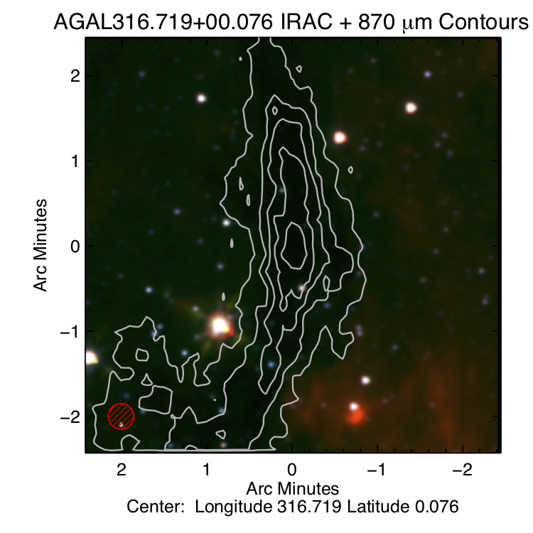 Figure 1
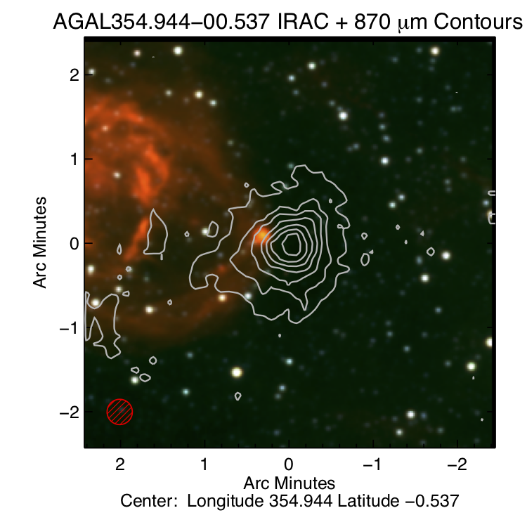 Figure 2
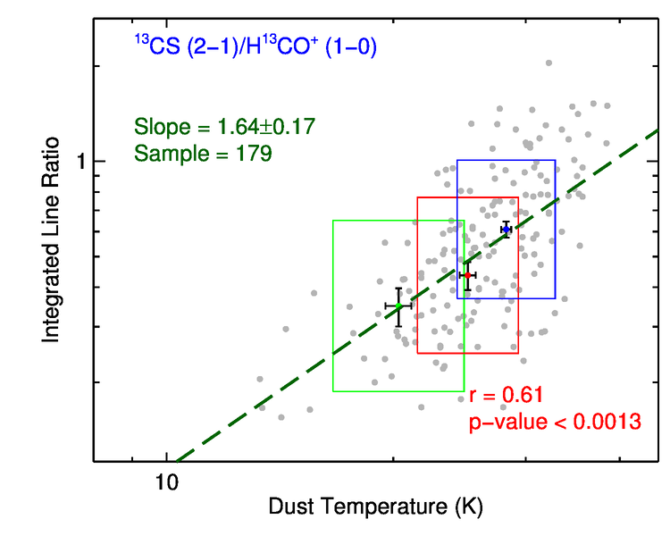 Figure 3
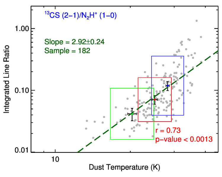 Figure 4
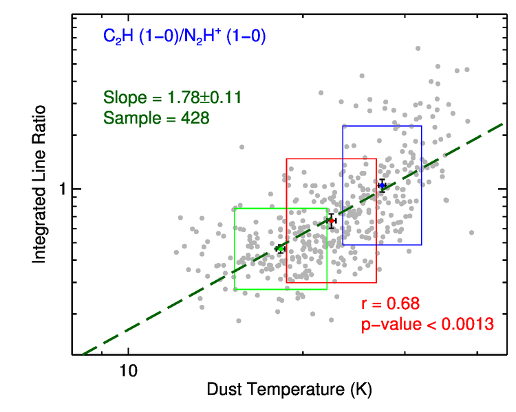 Figure 5
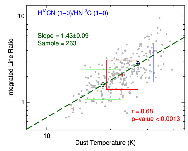 Figure 6
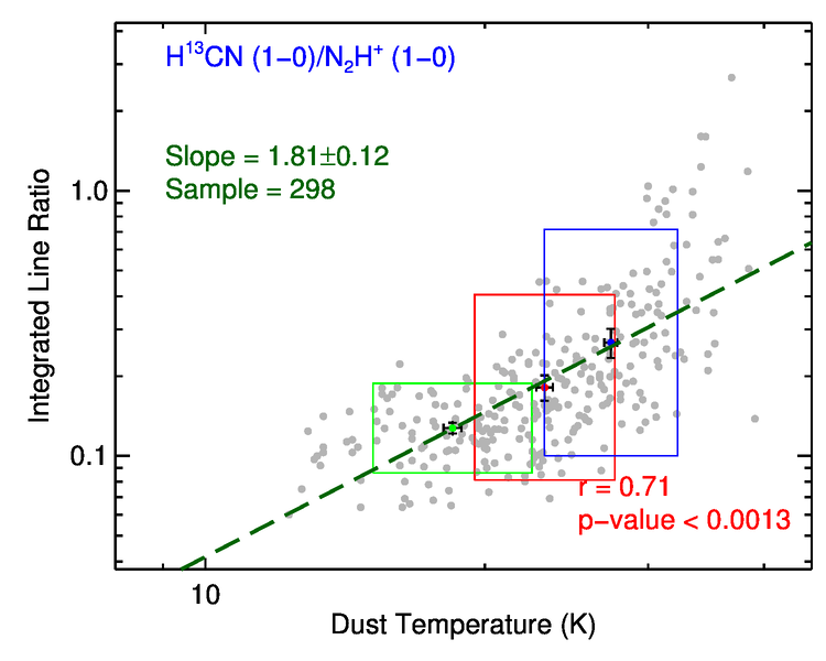 Figure 7
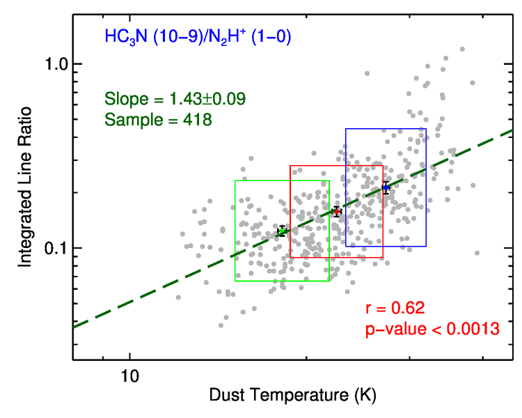 Figure 8
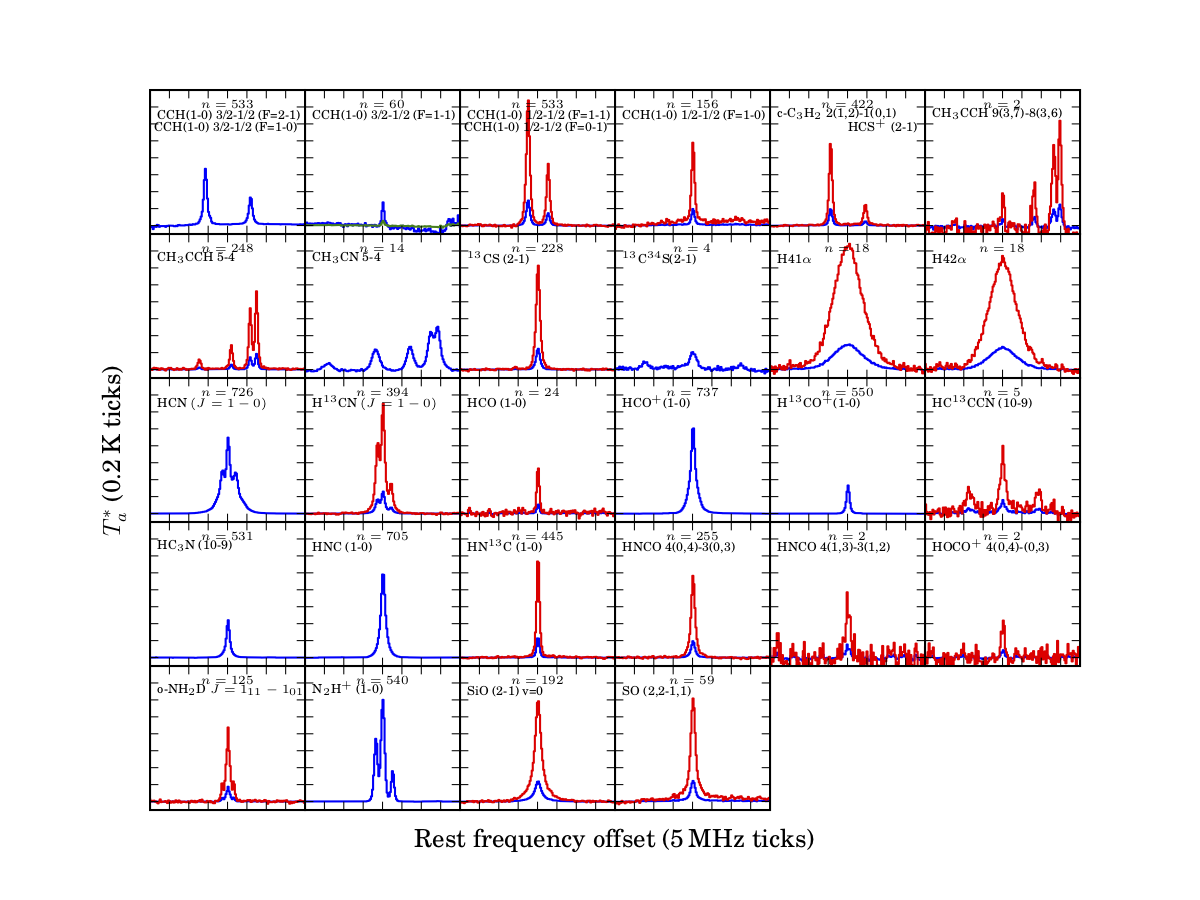 Figure 9
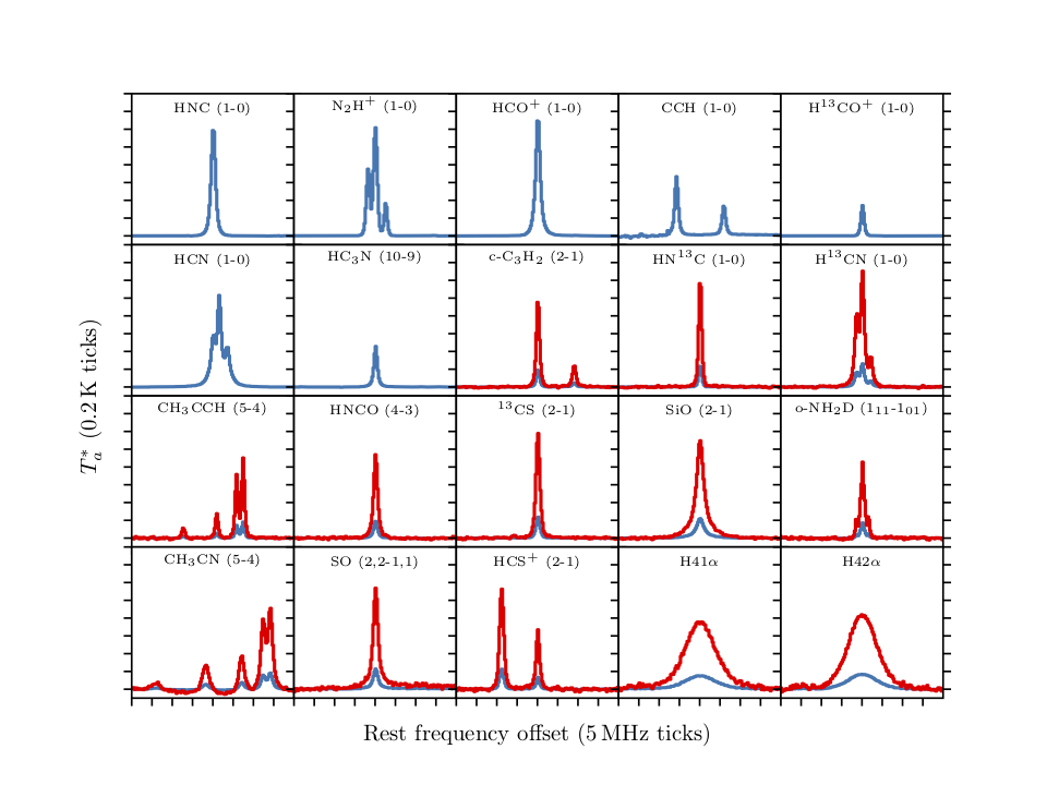 Figure 10
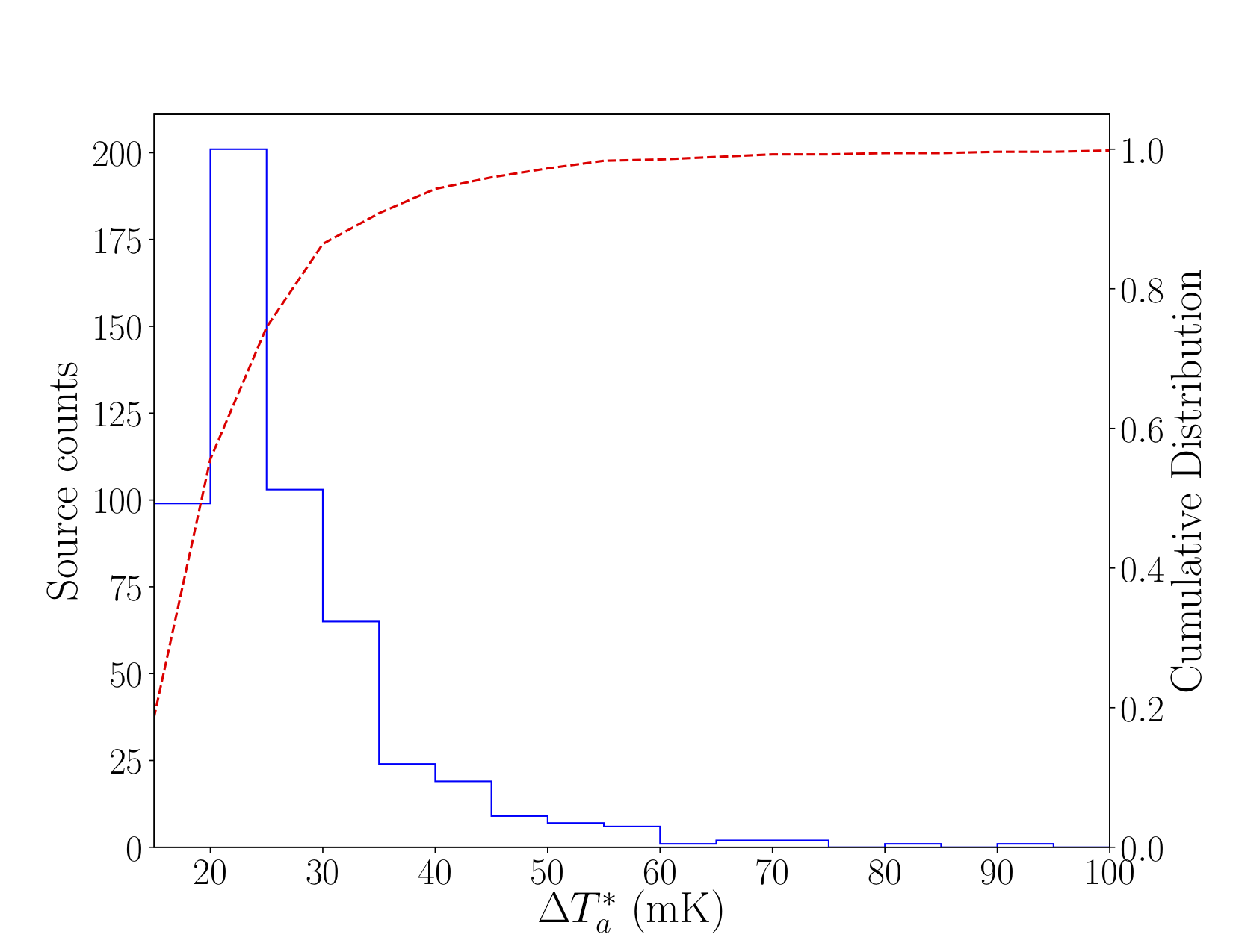 Figure 11
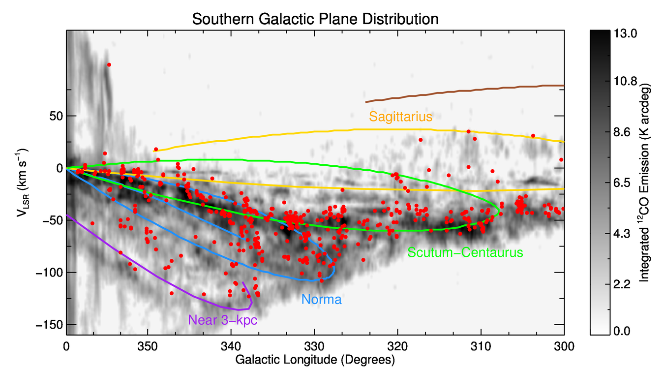 Figure 12
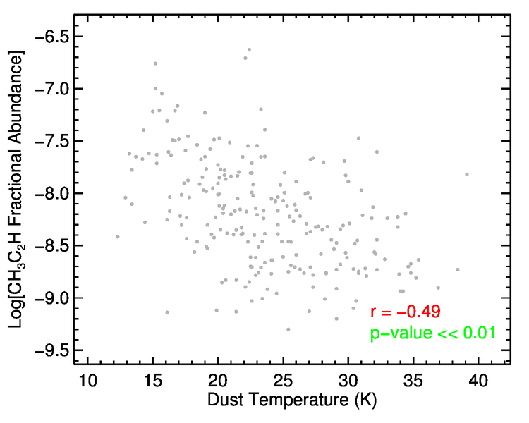 Figure 13
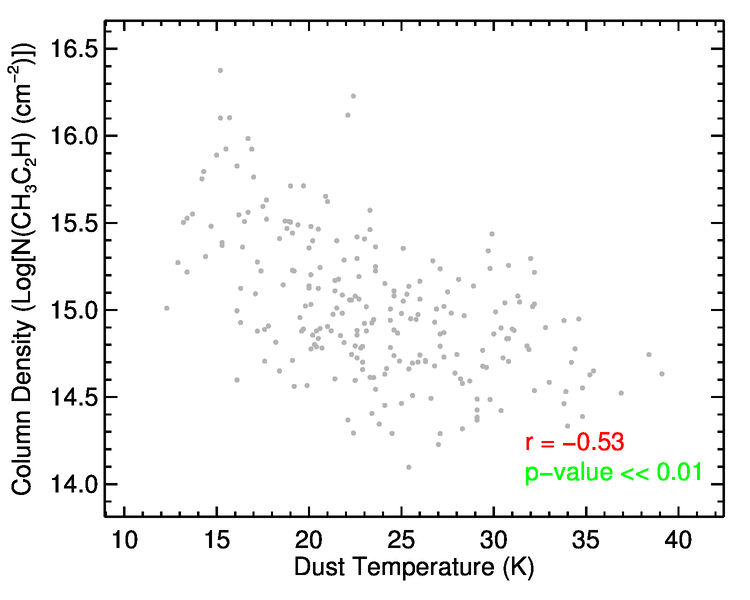 Figure 14
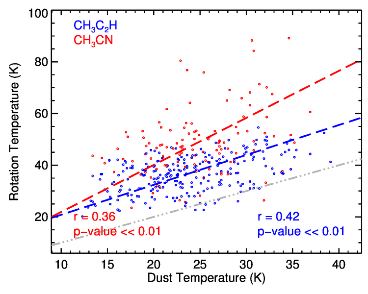 Figure 15
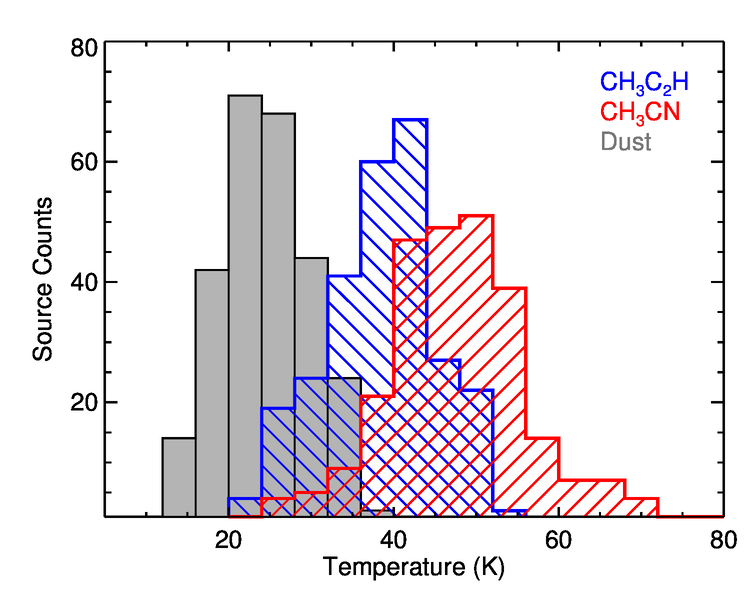 Figure 16
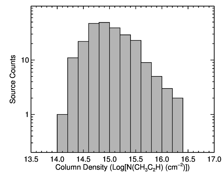 Figure 17
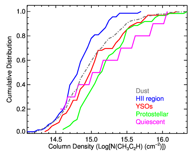 Figure 18
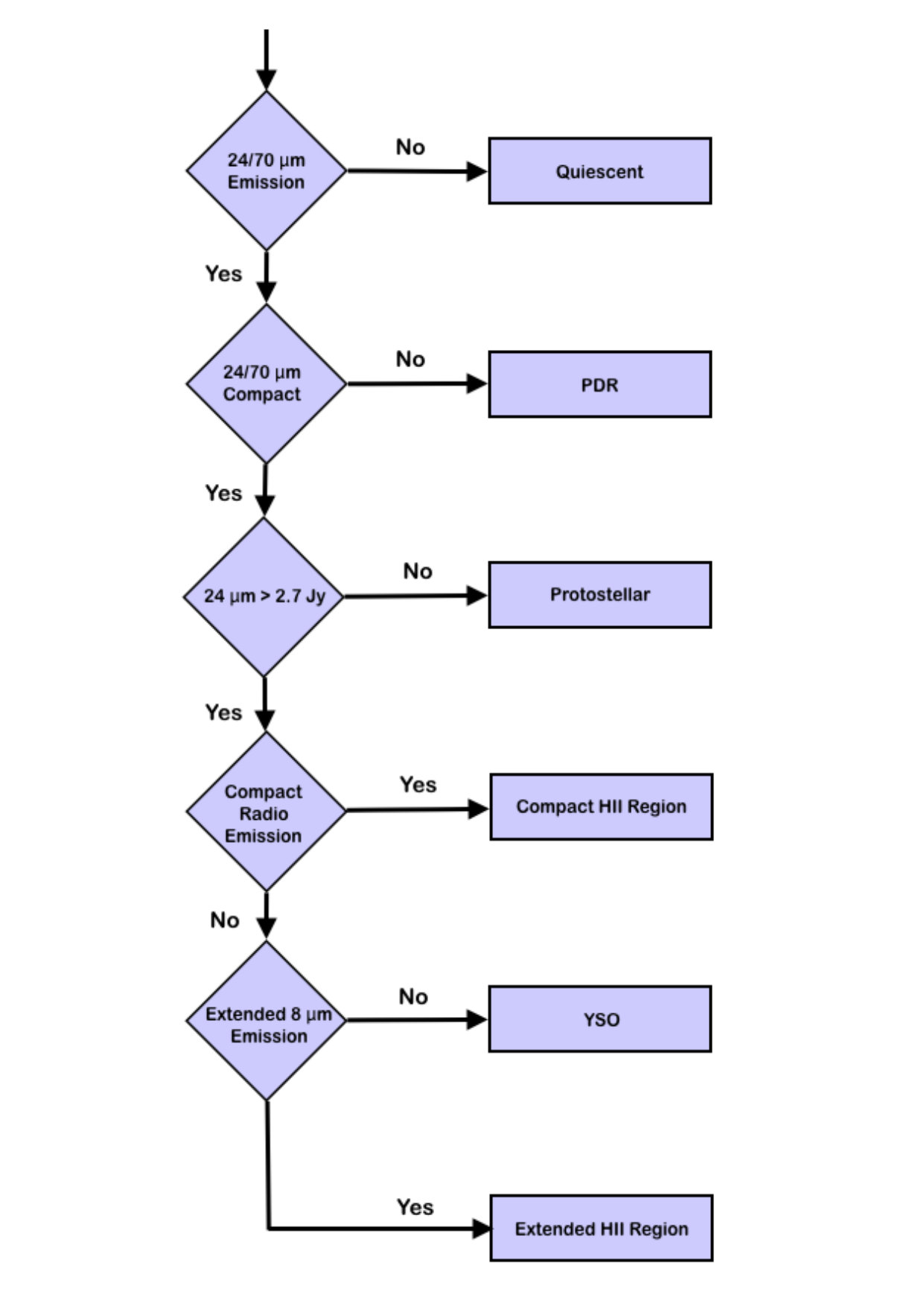 Figure 19
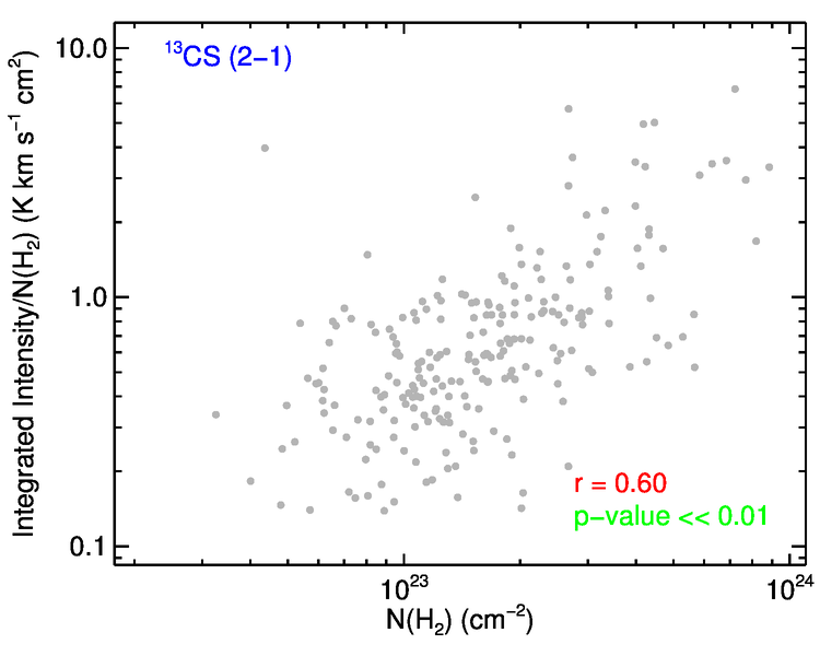 Figure 20
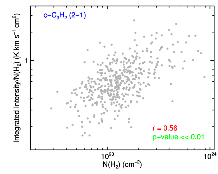 Figure 21
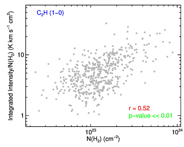 Figure 22
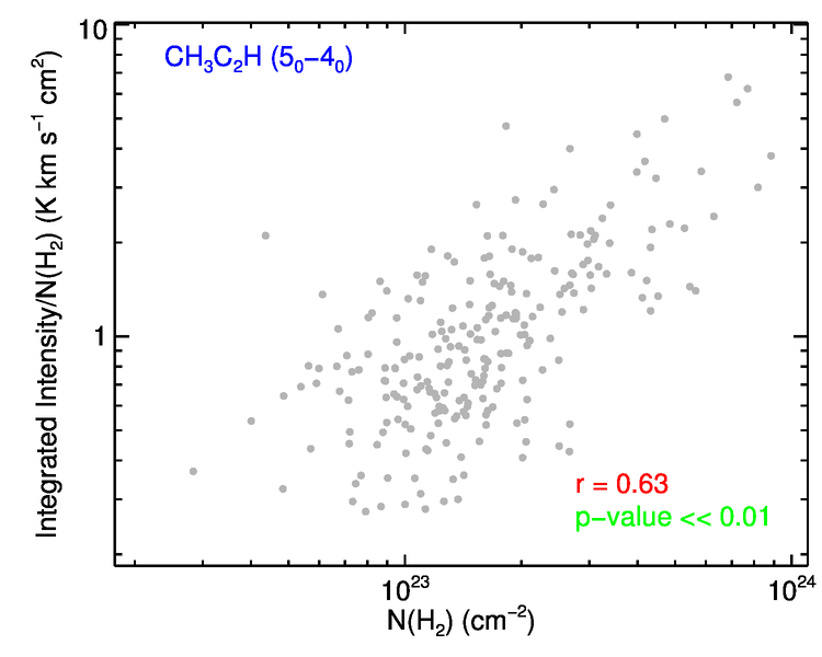 Figure 23
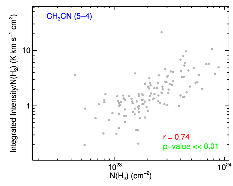 Figure 24
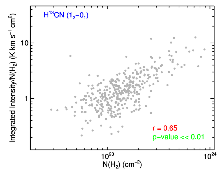 Figure 25
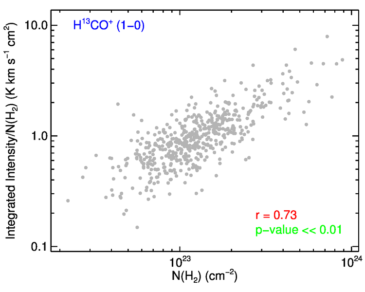 Figure 26
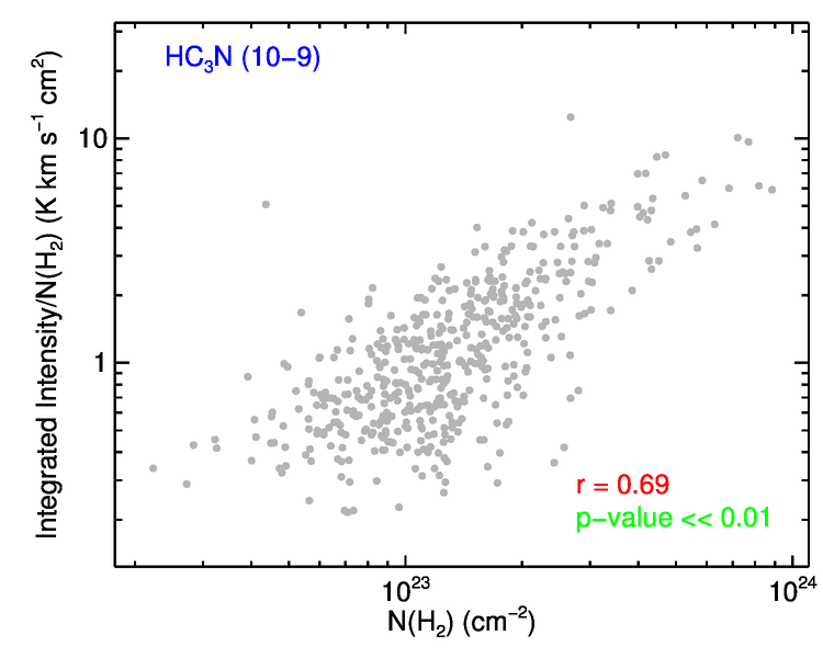 Figure 27
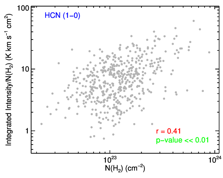 Figure 28
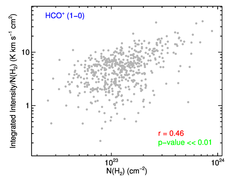 Figure 29
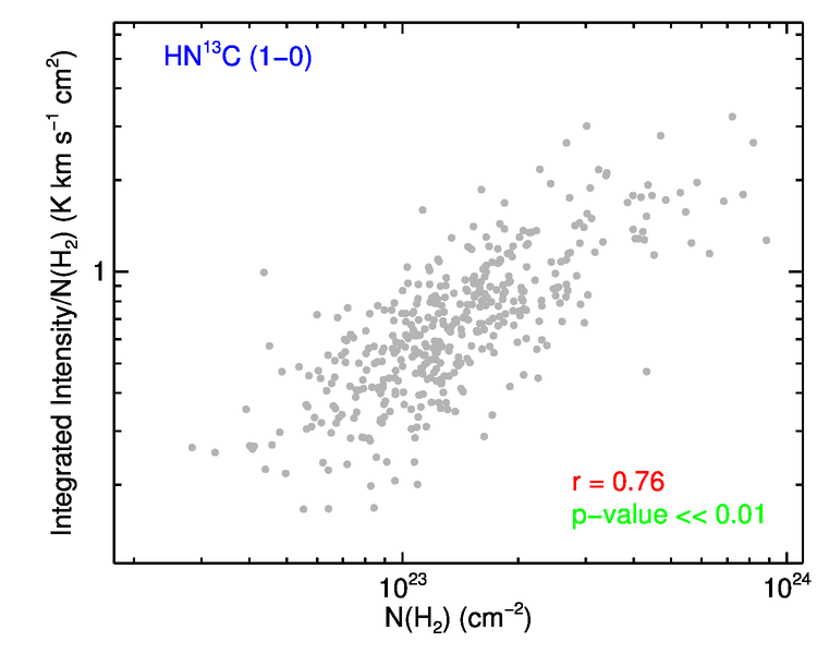 Figure 30
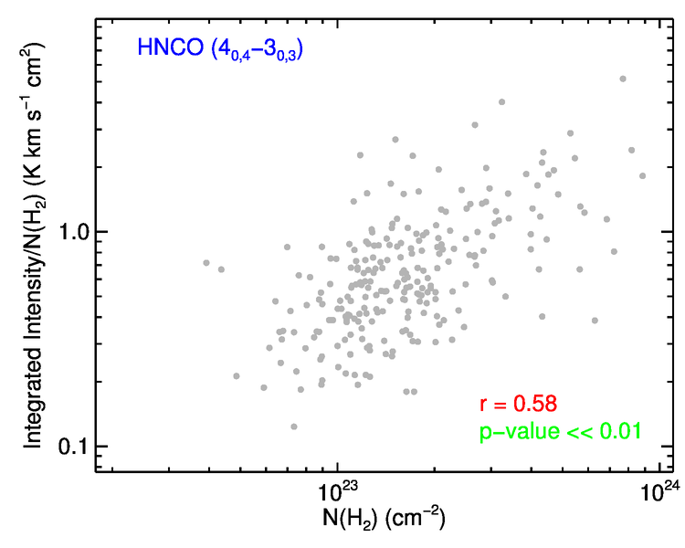 Figure 31
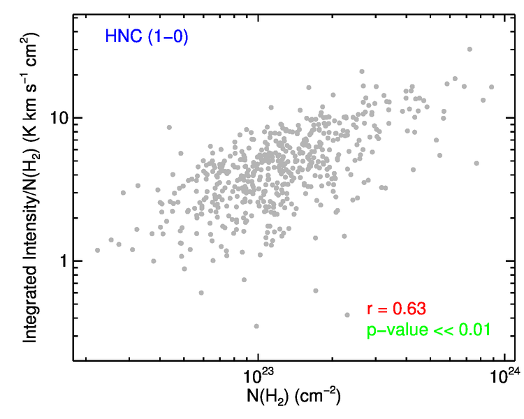 Figure 32
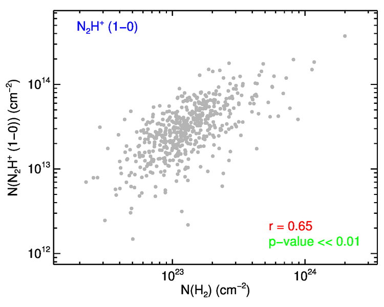 Figure 33
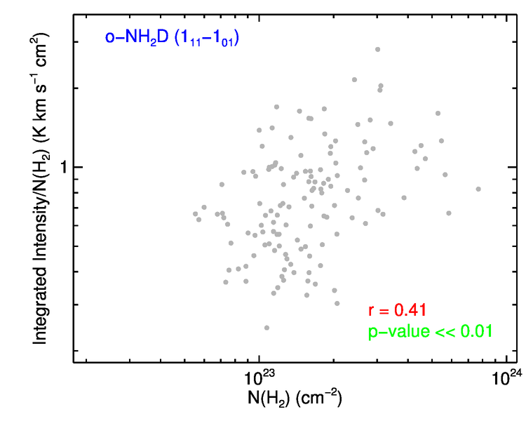 Figure 34
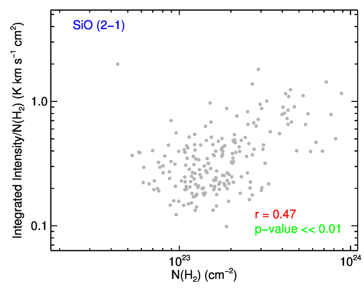 Figure 35
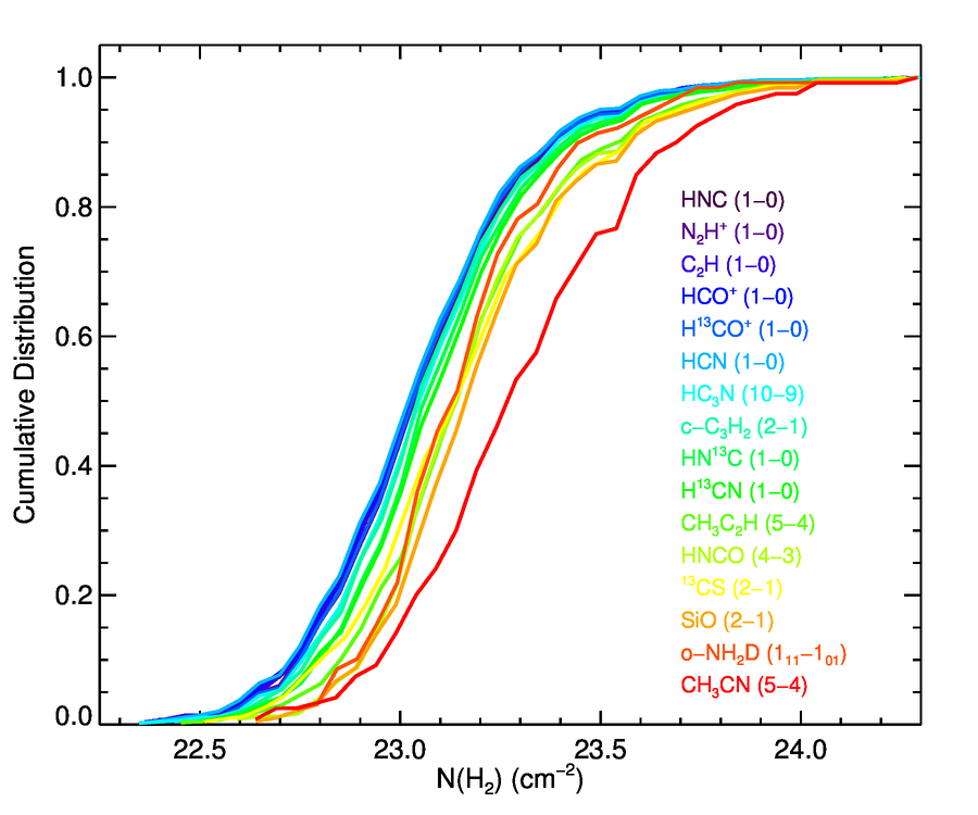 Figure 36
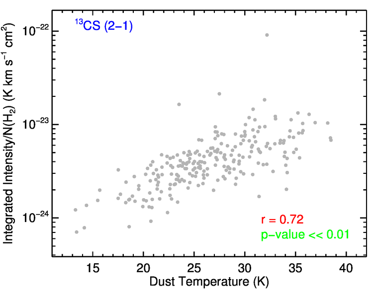 Figure 37
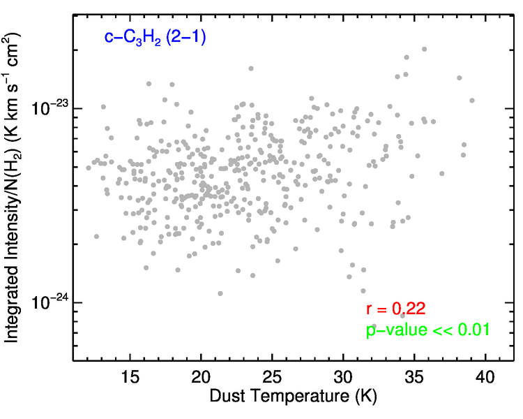 Figure 38
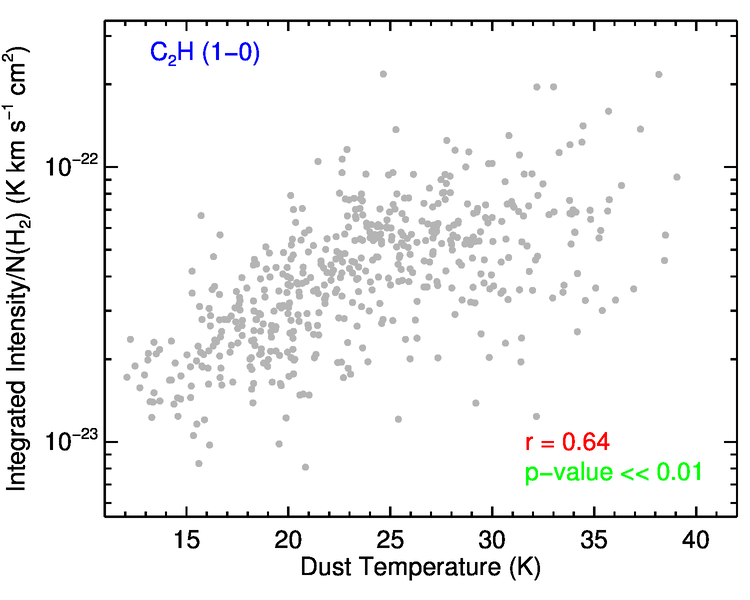 Figure 39
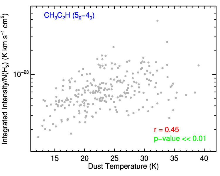 Figure 40
| ATLASGAL name | Classification | Offset | Distance | Log(M) | Log(L) | ||||
|---|---|---|---|---|---|---|---|---|---|
| (°) | (°) | (″) | (kpc) | (K) | (cm-2) | (M⊙) | (L⊙) | ||
| AGAL300.16400.087 | YSO | 4.300.95 | 18.891.39 | ||||||
| AGAL300.50400.176 | HII | 9.200.62 | 26.104.48 | ||||||
| AGAL300.721+01.201 | YSO | 3.400.91 | |||||||
| AGAL300.826+01.152 | Uncertain | 3.400.91 | 13.102.36 | ||||||
| AGAL300.911+00.881 | Protostellar | 3.400.91 | 23.594.38 | ||||||
| AGAL301.014+01.114 | Uncertain | 3.400.91 | 39.064.46 | ||||||
| AGAL301.116+00.959 | PDR | 3.400.91 | 20.873.34 | ||||||
| AGAL301.116+00.977 | PDR | 3.400.91 | 20.633.29 | ||||||
| AGAL301.13600.226 | HII | 4.601.14 | 34.171.20 | ||||||
| AGAL301.139+01.009 | Quiescent | 3.400.91 | 17.272.41 |
| Classification | Number | Log() | Log() | Log() | ||
|---|---|---|---|---|---|---|
| of clumps | (K) | (cm-2) | (M⊙) | (L⊙) | ||
| Quiescent | 29 | (5.1%) | 18.22.9 | 23.110.18 | 2.390.46 | 3.350.73 |
| Protostellar | 153 | (26.8%) | 18.73.3 | 23.100.25 | 2.580.57 | 3.400.75 |
| YSO | 128 | (22.5%) | 22.94.1 | 23.080.28 | 2.550.53 | 3.910.73 |
| Hii region | 166 | (29.1%) | 28.24.8 | 23.110.32 | 2.820.58 | 4.730.68 |
| PDR | 48 | (8.4%) | 27.44.7 | 23.030.21 | 2.370.43 | 4.420.69 |
| Uncertain | 46 | (8.1%) | 25.06.3 | 23.090.22 | 2.470.63 | 4.230.82 |
| Parameter | Value |
|---|---|
| Galactic longitude () range | 300° to 358.5° |
| Galactic latitude () )range | 1.15° to 1.58° |
| Number of observations | 601 |
| Number of CSCs observed | 570 |
| Frequency range | 85.2 GHz to 93.4 GHz |
| Angular resolution (FWHM)a | 362″ |
| Spectral resolution | 0.9 km s-1 |
| Typical noise (T) | 20-25 mK channel-1 |
| Typical system temperatures (T | 200 K |
| Typical pointing offset | 6″ |
| Integration time (on-source) | 15 mins |
| Main beam efficiency ()a | 0.49 |
| Mean observation offset | 7.8″ |
| Emission line(s) | Log() | Number of | Detection | RMS noise | Line-width | Intensity | Comments | ||||
|---|---|---|---|---|---|---|---|---|---|---|---|
| (GHz) | (K) | (cm-3) | detections | ratio | (mK) | (K) | (km s-1) | (km s-1 K) | |||
| (1) | (2) | (3) | (4) | (5) | (6) | (7) | (8) | (9) | (10) | (11) | |
| c-C3H2 (2-1) | 85.3389 | 6.0 | 446 | (9) | 0.78 | 24 | 0.21 | 3.3 | 0.72 | Cyclic molecules | |
| HCS+ (2-1) | 85.3479 | 4.5 | 62 | (0) | 0.11 | 22 | 0.13 | 3.3 | 0.49 | Sulphur chemistry | |
| CH2CHCN (9-8) | 85.4218 | 3 | (0) | 0.01 | 28 | 0.11 | 1.2 | 0.19 | Temperature | ||
| CH3C2H (5-4) | 85.4573 | 273 | (4) | 0.48 | 26 | 0.19 | 2.8 | 1.34 | Temperature | ||
| HOCO+ (404-403) | 85.5315 | 5.2 | 3 | (0) | 0.01 | 17 | 0.08 | 4.5 | 0.4 | Indirect gas-phase CO2 tracer | |
| H42 | 85.6884 | 58 | (1) | 0.10 | 11 | 0.16 | 27.6 | 1.03 | Ionised gas | ||
| o-NH2D (111-101) | 85.9263 | 6.6 | 148 | (0) | 0.26 | 24 | 0.15 | 2.1 | 0.89 | Deuteration, coldest dense gas | |
| SO () | 86.0940 | 5.2 | 67 | (0) | 0.12 | 26 | 0.31 | 5.2 | 4.64 | Suphur chemistry, shocks | |
| H13CN (1-0) | 86.3402 | 6.3 | 403 | (13) | 0.71 | 26 | 0.25 | 3.5 | 2.03 | Dense gas | |
| HCO (1-0) | 86.6708 | 36 | (0) | 0.06 | 22 | 0.11 | 2.8 | 0.35 | Photon dominated regions | ||
| H13CO+ (1-0) | 86.7543 | 4.8 | 536 | (20) | 0.94 | 25 | 0.36 | 3.1 | 1.2 | Dense gas | |
| SiO (2-1) | 86.8470 | 5.4 | 218 | (9) | 0.38 | 10 | 0.17 | 13.2 | 0.45 | Shocks, outflows | |
| HN13C (1-0) | 87.0908 | 5.5 | 445 | (7) | 0.78 | 26 | 0.26 | 3.1 | 0.82 | Dense gas | |
| C2H (1-0) | 87.3169 | 6.0 | 542 | (131) | 0.95 | 45 | 0.68 | 3.5 | 6.31 | Early chemistry/PDRb | |
| HNCO (4-3) | 87.9253 | 6.0 | 269 | (1) | 0.47 | 25 | 0.19 | 3.8 | 0.82 | Hot core, FIR, chemistry | |
| HCN (1-0) | 88.6318 | 5.7 | 528 | (284) | 0.93 | 34 | 0.98 | 4.5 | 9.15 | Dense gas | |
| HCO+ (1-0) | 89.1885 | 4.8 | 542 | (136) | 0.95 | 39 | 1.34 | 4.5 | 6.26 | Kinematics (Infall, outflow) | |
| HNC (1-0) | 90.6636 | 5.1 | 562 | (119) | 0.99 | 33 | 1.24 | 4.2 | 5.54 | High column density, cold gas tracer | |
| C2S (2-1) | 90.6864 | 3 | (0) | 0.01 | 21 | 0.09 | 3.8 | 0.31 | Dense gas, evolutionary phase | ||
| 13C34S (2-1) | 90.9260 | 5.6 | 2 | (0) | 0.00 | 25 | 0.11 | 2.8 | 0.34 | Column density | |
| HC3N (10-9) | 90.9790 | 5.0 | 514 | (22) | 0.90 | 26 | 0.46 | 3.1 | 1.64 | Hot core | |
| HC13C2N (10-9) | 90.9790 | 5.2 | 3 | (0) | 0.01 | 22 | 0.12 | 12.7 | 1.31 | Hot core | |
| CH3CN (5-4) | 91.9871 | 5.4 | 142 | (5) | 0.25 | 25 | 0.18 | 4.5 | 2.74 | Hot core temperature | |
| H41 | 92.0345 | 60 | (0) | 0.11 | 10 | 0.14 | 31.8 | 0.92 | Ionised gas | ||
| 13CS (2-1) | 92.4943 | 5.5 | 250 | (1) | 0.44 | 23 | 0.24 | 3.5 | 0.95 | Dense gas, infall | |
| N2H+ (1-0) | 93.1738 | 4.8 | 545 | (0) | 0.96 | 27 | 0.66 | 3.1 | 8.62 | Dense gas, depletion resistant | |
| ATLASGAL | Transition | RMS | VLSR | VLSR error | error | VLSR | VLSR error | Intensity | |
|---|---|---|---|---|---|---|---|---|---|
| CSC name | (mK) | (km s-1) | (km s-1) | (K) | (K) | (km s-1) | (km s-1) | (K km s-1) | |
| AGAL300.16400.087 | N2H+ (1-0) | ||||||||
| AGAL300.50400.176 | N2H+ (1-0) | ||||||||
| AGAL300.721+01.201 | N2H+ (1-0) | ||||||||
| AGAL300.826+01.152 | N2H+ (1-0) | ||||||||
| AGAL300.911+00.881 | N2H+ (1-0) | ||||||||
| AGAL301.014+01.114 | N2H+ (1-0) | ||||||||
| AGAL301.116+00.959 | N2H+ (1-0) | ||||||||
| AGAL301.116+00.977 | N2H+ (1-0) | ||||||||
| AGAL301.13600.226 | N2H+ (1-0) | ||||||||
| AGAL301.139+01.009 | N2H+ (1-0) |
| Temperature | Column density | Linewidth | Velocity | |
|---|---|---|---|---|
| [K] | [log(cm-2)] | [km s-1] | [km s-1] | |
| Prior | Truncated normal | Normal | Truncated normal | Normal |
| Parameters (cool) | K | |||
| CSC Name | CH3C2H | CH3CN | SiO | Notes1 |
|---|---|---|---|---|
| AGAL316.719+00.076 | X | Quiescent | ||
| AGAL326.652+00.619 | X | X | X | Quiescent/PDR |
| AGAL331.02900.431 | X | Quiescent/PDR | ||
| AGAL331.639+00.501 | X | Quiescent | ||
| AGAL333.01400.521 | X | Quiescent/PDR | ||
| AGAL333.07100.399 | X | Quiescent/PDR | ||
| AGAL333.52400.269 | X | Quiescent/PDR | ||
| AGAL338.459+00.024 | X | X | Quiescent | |
| AGAL351.466+00.682 | X | X | X | Quiescent/PDR |
| AGAL351.571+00.762 | X | Quiescent/PDR | ||
| AGAL354.94400.537 | X | Quiescent/PDR |
| Parameter | # | ||||||
|---|---|---|---|---|---|---|---|
| Log[(CH3C2H) (cm-2)] | 240 | ||||||
| Hii region | 68 | ||||||
| YSO | 66 | ||||||
| Protostellar | 61 | ||||||
| Quiescent | 10 | ||||||
| Log[(CH3CN) (cm-2)] | 121 | ||||||
| HII | 40 | ||||||
| YSO | 66 | ||||||
| Protostellar | 34 | ||||||
| Quiescent | 3 |
| Intensity | Line-width | |||||||||
|---|---|---|---|---|---|---|---|---|---|---|
| post-hoc tests | post-hoc tests | |||||||||
| Line Ratio | Test | Test | ||||||||
| (1) | (2) | (3) | (4) | (5) | (6) | (7) | (8) | (9) | (10) | (11) |
| H13CN/N2H+ | Kruskal-Wallis | 0.000 | 1.000 | 0.000 | 0.000 | Kruskal-Wallis | 0.062 | |||
| 13CS/N2H+ | Kruskal-Wallis | 0.000 | 1.000 | 0.018 | 0.000 | ANOVA | 0.930 | |||
| HCN/HNC | ANOVA | 0.000 | 0.900 | 0.036 | 0.039 | Kruskal-Wallis | 0.017 | 0.417 | 1.000 | 1.000 |
| HCN/N2H+ | Kruskal-Wallis | 0.000 | 1.000 | 0.002 | 0.001 | Kruskal-Wallis | 0.099 | |||
| HC3N/HN13C | ANOVA | 0.000 | 0.598 | 0.004 | 0.001 | Kruskal-Wallis | 0.002 | 0.768 | 0.223 | 1.000 |
| H13CN/HN13C | Kruskal-Wallis | 0.000 | 1.000 | 0.001 | 0.000 | ANOVA | 0.850 | |||
| HC3N/N2H+ | Kruskal-Wallis | 0.000 | 0.275 | 0.001 | 0.000 | ANOVA | 0.004 | 0.003 | 0.900 | 0.900 |
| CCH/N2H+ | Kruskal-Wallis | 0.000 | 0.181 | 0.000 | 0.000 | Kruskal-Wallis | 0.000 | 0.436 | 0.014 | 0.838 |
| HCO+/N2H+ | Kruskal-Wallis | 0.000 | 1.000 | 0.009 | 0.020 | ANOVA | 0.319 | |||
| H13CO+/N2H+ | Kruskal-Wallis | 0.000 | 1.000 | 0.000 | 0.019 | ANOVA | 0.000 | 0.444 | 0.001 | 0.900 |
| H13CO+/HN13C | ANOVA | 0.000 | 0.249 | 0.008 | 0.033 | Kruskal-Wallis | 0.221 | |||
| CCH/HN13C | ANOVA | 0.000 | 0.092 | 0.012 | 0.001 | ANOVA | 0.106 | |||
| CCH/c-C3H2 | Kruskal-Wallis | 0.000 | 1.000 | 0.000 | 0.011 | ANOVA | 0.000 | 0.806 | 0.122 | 0.900 |
Peer Reviews
No public reviews on file for this paper yet. If you reviewed it on a platform where reviews are public (OpenReview, ICLR, NeurIPS, ICML), you can paste yours below so the community can read it here.
Videos
No videos yet. Explain this paper in a talk, walkthrough, or lecture? Add one.
ATLASGAL — Molecular fingerprints of a sample
of massive star forming clumps††thanks: The full version of Tables 1, 5 and LABEL:table:integrated_intensities are only available in electronic form at the CDS via anonymous ftp to cdsarc.u-strasbg.fr (130.79.125.5) or via http://cdsweb.u-strasbg.fr/cgi-bin/qcat?J/MNRAS/.
J. S. Urquhart1,2, C. Figura3, F. Wyrowski2, A. Giannetti4,2, W.-J. Kim2, M. Wienen2, S. Leurini5,2, T. Pillai2, T. Csengeri2, S. J. Gibson1, K. Menten2, T. J. T. Moore6,M. A. Thompson7
1 Centre for Astrophysics and Planetary Science, University of Kent, Canterbury, CT2 7NH, UK
2 Max-Planck-Institut für Radioastronomie, Auf dem Hügel 69, D-53121 Bonn, Germany
3 Wartburg College, Waverly, IA, 50677, USA
4 INAF - Istituto di Radioastronomia & Italian ALMA Regional Centre, Via P. Gobetti 101, I-40129 Bologna, Italy
5 INAF - Osservatorio Astronomico di Cagliari, Via della Scienza 5, I-09047, Selargius (CA), Italy
6 Astrophysics Research Institute, Liverpool John Moores University, Liverpool Science Park, 146 Brownlow Hill, Liverpool, L3 5RF, UK
7 Science and Technology Research Institute, University of Hertfordshire, College Lane, Hatfield, AL10 9AB, UK E-mail: [email protected]
(Accepted XXX. Received YYY; in original form ZZZ)
Abstract
We have conducted a 3-mm molecular-line survey towards 570 high-mass star-forming clumps, using the Mopra telescope. The sample is selected from the 10,000 clumps identified by the ATLASGAL survey and includes all of the most important embedded evolutionary stages associated with massive star formation, classified into five distinct categories (quiescent, protostellar, young stellar objects, Hii regions and photo-dominated regions). The observations were performed in broadband mode with frequency coverage of 85.2 to 93.4 GHz and a velocity resolution of 0.9 km s*-1*, detecting emission from 26 different transitions. We find significant evolutionary trends in the detection rates, integrated line intensities, and abundances of many of the transitions and also identify a couple of molecules that appear to be invariant to changes in the dust temperature and evolutionary stage (N2H+ (1-0) and HN13C (1-0)). We use the K-ladders for CH3C2H (5-4) and CH3CH (5-4) to calculate the rotation temperatures and find 1/3 of the quiescent clumps have rotation temperatures that suggest the presence of an internal heating source. These sources may constitute a population of very young protostellar objects that are still dark at 70 m and suggest that the fraction of truly quiescent clumps may only be a few per cent. We also identify a number of line ratios that show a strong correlation with the evolutionary stage of the embedded objects and discuss their utility as diagnostic probes of evolution.
keywords:
Stars: formation – Stars: early-type – ISM: clouds – ISM: submillimetre – ISM: Hii regions.
††pubyear: 2017††pagerange: ATLASGAL — Molecular fingerprints of a sample of massive star forming clumps††thanks: The full version of Tables 1, 5 and are only available in electronic form at the CDS via anonymous ftp to cdsarc.u-strasbg.fr (130.79.125.5) or via http://cdsweb.u-strasbg.fr/cgi-bin/qcat?J/MNRAS/.–LABEL:lastpage
1 Introduction
Massive stars play a dominant role in the evolution of galaxies through the release of vast amounts of radiative and mechanical energy (e.g., jets, molecular outflows and powerful stellar winds) into the interstellar medium (ISM). They are responsible for the production of nearly all of the heavy elements, which are returned to the ISM in the late stages of their evolution, or at the time of their death via supernova explosions. The enrichment of the ISM and the energy pumped into their local environments change the chemical composition and structure of the surrounding gas, which can have a significant impact on future star formation activity: this can lead to an enhancement of the local star formation rate (such as triggering; Urquhart et al. 2007) or can result in the disruption of molecular material before star formation has a chance to begin. Massive stars can, therefore, play an important role in shaping their local environments and regulating star formation.
Due to their short lifetime, massive stars do not escape significantly from their birth places. Observations of nearby spiral galaxies have revealed a tight correlation between spiral arms and the locations of massive star formation, and so the spatial distribution of massive stars in our own Galaxy can help us derive the structure and dynamics of the Milky Way. These points taken together indicate that understanding the formation and evolution of massive stars is therefore of crucial importance to many areas of astrophysics. At present, there is no well-established evolutionary scheme for high mass star formation, in contrast to the detailed framework of classes that exists for the early evolution of low-mass stars. In the 1990s, targeted surveys found many ultracompact Hii regions (Wood & Churchwell, 1989), and hot molecular cores were found to be associated with them in subsequent follow-up observations (e.g. Cesaroni et al., 1992). More recently, so called high-mass protostellar objects (HMPOs) or massive young stellar objects (MYSOs) were recognized as likely to represent an even earlier stage of massive star formation (e.g. Beuther et al., 2002; Lumsden et al., 2013). Infra-red dark clumps have also been found to be promising candidates for even earlier stages in the formation of massive stars (see Yuan et al., 2017, and references therein).
These targeted surveys are, however, only partial, as they usually only trace one of the stages of massive star formation (MSF); UC Hii regions, massive young stellar objects (MYSOs) or CH3OH masers and infrared darks clouds (e.g. Egan et al. 1998; Simon et al. 2006; Peretto & Fuller 2009) for instance. As a result, they may miss entire classes of objects, or have very incomplete statistics. In contrast, an unbiased sample using complete dust continuum imaging at the scale of the molecular complex Cygnus-X (Motte et al., 2007) was able to derive some more systematic results on the existence of a cold phase for high-mass star formation. To remedy this situation, APEX/LABOCA was used to produce the first unbiased submillimetre continuum survey of the inner Galactic plane.
In this paper we will use a molecular line survey of 600 massive clumps that include examples of all evolutionary stages associated with high-mass star formation in an effort to identify trends that might be utilised to develop a chemical clock for massive star formation. There have already been some efforts to address this recently with chemical evolution studies towards samples of IRDCs (e.g., Sanhueza et al. 2012; Sakai et al. 2010) and massive clump selected from their dust emission (e.g., Hoq et al. 2013; Rathborne et al. 2016). These have identified trends in specific line ratios and abundances, however, these have either been limited in the number of sources or in sensitivity and so we aim to build on these findings of these previous studies.
1.1 ATLASGAL – The APEX/LABOCA Galactic plane survey
The APEX Telescope Large Area Survey of the Galaxy (ATLASGAL) is an unbiased 870 m submillimetre survey covering 420 sq. degrees of the inner Galactic plane (Schuller et al. 2009). The regions covered by this survey are with and with between 2° and 1°; the change in latitude was necessary to account for the warp in the Galactic disc in the outer Galaxy extension.
Only a large unbiased survey can provide the statistical base to study the scarce and short-living protoclusters as the origin of the massive stars and the richest clusters in the Galaxy. The dust continuum emission in the (sub)millimetre range is the best tracer of the earliest phases of (high-mass) star formation since it is directly probing the material from which the stars form. Cross-correlation with other complementary Galactic plane continuum surveys (e.g., GLIMPSE (Benjamin et al., 2003); MSX (Price et al., 2001); WISE (Wright et al., 2010); MIPSGAL (Carey et al., 2009); HiGAL (Molinari et al., 2010a); and CORNISH (Hoare et al., 2012)) and molecular line surveys (e.g., CHIMPS (Rigby et al., 2016); SEDIGISM (Schuller et al., 2017); HOPS (Walsh et al., 2011); and the MMB survey (Caswell, 2010)) will help considerably to answer a wide range of questions including: (1) What are the properties of the cold phase of massive star-formation? (2) What is the evolutionary sequence for high-mass stars? (3) How important is triggering to form new generations of high-mass stars? (4) What are the earliest phases of the richest clusters of the Galaxy?
Source extraction has identified 10,000 distinct massive clumps (Contreras et al. 2013; Urquhart et al. 2014a; Csengeri et al. 2014). Analyses by Wienen et al. (2015) of the physical properties of these clumps revealed that 92 per cent satisfy the Kauffmann et al. (2010) size-mass criterion for massive star formation. Furthermore, the majority (90 per cent) of these clumps also are already associated with star formation (i.e., hosting an embedded 70 m point source; Urquhart et al. 2018). Further analysis has confirmed that 15% of these infrared bright sources are associated with massive young stellar objects and compact Hii regions (e.g., Urquhart et al. 2013a, b, 2014b). Only a small fraction appear to be in a quiescent phase (15 per cent; Urquhart et al. 2018) and are therefore likely to be cold precursors to massive protostars. This is probably an upper limit as some of these have been found to be associated with outflows (Feng et al. 2016; Tan et al. 2016 and Yang et al. 2017) and, as we will find from rotation temperature calculations, many more appear to host an internal heating source.
1.2 Molecular fingerprints with Mopra
Large scale continuum surveys are crucial for the study of massive star formation but there are a couple of shortcomings: perhaps the most significant is that, a priori, the distances to the newly found sources, which are needed to determine important parameters such as mass and luminosity of the clumps, are unknown. Furthermore, their dust temperatures and densities are only loosely constrained by spectral energy distributions (in conjunction with infrared surveys). However, all of these issues can be more tightly constrained by molecular line observations, such as NH3, CH3C2H and CH3CN, of the massive star forming regions (e.g., Urquhart et al. 2011; Wienen et al. 2015; Tang et al. 2017; Giannetti et al. 2017).
We have embarked on a project to use the high sensitivity and large bandwidth of the Mopra telescope to study the physical and chemical properties of a large and unbiased sample of Galactic massive star forming clumps. The results from this Mopra survey are vital for the analysis of the Galactic plane survey, since they allow us to investigate the kinematic, thermal and chemical properties of the clumps. These can be thought of as the “molecular fingerprints” of the dust clumps and allow us to determine their kinematic distances, virial masses, infall and outflow activity, as well as probing their temperature, density and chemistry.
In this paper we present an overview of the Mopra spectral line survey and discuss the statistical properties of the sample. Detailed analysis of individual transitions is ongoing and will be published separately, and some of the transitions have already been published (e.g., mm-radio recombination lines — Kim et al. 2017; temperature determination — Giannetti et al. 2017). Furthermore, the line velocities have been used to derive distances, and aperture photometry has been performed on MSX/WISE and HiGAL and ATLASGAL emission maps to fit their spectral energy distributions to estimate clump bolometric luminosities, dust temperatures and masses (see König et al. 2017 and Urquhart et al. 2018 for more details). The observational data have been used to construct an evolutionary sequence for the formation of massive stars. Here, we examine the molecular line detection rates and fitted properties to see if they are consistent with this sequence and whether they can provide a deeper insight into the processes involved.
The structure of the paper is as follows: in Sect. 2 we outline the source selection criteria, in Sect. 3 we describe the observational set up and the data reduction methodology. Sect. 4 presents the results and discusses the overall statistical properties of the sample. We discuss the viability of using these molecular transitions to trace the evolution of the ongoing embedded star formation in Sect. 5. In Sect. 6 we present a summary of our results and highlight our main findings.
2 Source selection
We have selected a flux-limited sample of clumps (2 Jy beam*-1* for clumps associated with MSX 21 m point sources ( Jy) and 1 Jy beam*-1* for mid-infrared weak sources ( Jy) due to their lower temperatures)111Clumps associated with mid-infrared sources have dust temperatures between 20 and 30 while less evolved clumps have temperature between 10 and 20 K; the difference in temperature results in the clumps associated with embedded objects being a factor of 2 brighter at submillimetre wavelengths than clumps where the star formation is less evolved. , ensuring sufficiently high column densities for the Mopra line detections and coverage of all stages of massive star formation. As shown in Fig. 3, we consider all sources without a clear MSX 21-m point source coincident within 10″ of the peak submillimetre emission to be quiescent or in the very earliest stages of star formation. We are able to probe all massive clumps down to a mass limit of 100 within 5 kpc, which is the distance of the Galactic molecular ring.
A total 600 sources that satisfied the selection criteria and are located in the Galactic longitude range and latitude were observed as part of this line survey. These were drawn from a preliminary version of the catalogue produced using a Gaussian source-finder from an early reduction of the maps. A consequence of this is that a small number of the observed sources were spurious detections (9 sources corresponding to 2 per cent of the sample) and do not appear in the final ATLASGAL Compact Source Catalogue (CSC; Contreras et al. 2013; Urquhart et al. 2014c).
Another consequence was that the peak positions were not always well-constrained, and this has led to offsets between the peak of the submillimetre emission and the telescope point position; these offsets are shown in Fig. 1. The resolution and pointing accuracy of the Mopra telescope is 36″ and 6″, respectively. We use a value of 20″ (approximately half of the Mopra beam) to match the spectral emission features with the ATLASGAL clumps: this reduces the sample to 570 clumps, which corresponds to 95 per cent of the observed sources.
In Fig. 2, we show the peak flux distribution of the reduced sample (yellow hatching) and all of the ATLASGAL CSC sources in the same region of the sky. This plot shows that this sample is almost complete for all bright clumps located in the fourth quadrant above 2 Jy beam*-1*, and is therefore representative of the Galactic population of bright clumps. It is this reduced sample of 570 clumps that will be the focus of this paper.
These sources have been classified using the method and criteria used to classify the ATLASGAL Top 100 sample (König et al. 2017 and Urquhart et al. 2018) into four evolutionary types: quiescent, protostellar, YSO and Hii regions. The Hii regions and YSOs have similar mid-infrared colours and appear similar in mid-infrared images, and so we use the presence of compact radio continuum emission to classify compact Hii regions while extended 8-m emission identifies more evolved Hii emission regions. Following Jackson et al. (2013), we also include an additional classification to identify clumps located towards the edges of more evolved Hii regions, where the chemistry of these clumps and their structure are likely to be driven by the photo-dominated region (PDR). While the quiescent, protostellar, YSO and Hii regions are an observationally defined evolutionary sequence for embedded stars, the PDRs are driven by much more evolved stars that have emerged from their natal environment. We include the PDRs in the plots and note any interesting trends for completeness and to facilitate comparison with other studies (e.g., Rathborne et al. 2016), however, we refrain from including these sources in any of the detailed analyses presented in this study.
We present a flowchart that outlines the classification scheme in Fig. 3. Individual source classifications and physical properties are summarised in Table 1. The distances, dust temperatures and their uncertainties are taken from Urquhart et al. (2018) while the column densities and masses have been recalculated using the 870-m flux measured using a 36″ aperture centred on the Mopra position. The measurement uncertainties (i.e., distance, flux and temperature) in the masses and column densities are between 20-40 per cent, however, these are dominated by uncertainties in the dust to gas ratio and dust opacity. We therefore do not explicitly give the uncertainties for these parameters in Table 1 but estimate the mass and column densities to be correct within a factor of two. The uncertainty in the luminosity is a combination of the distance and flux measurements used for the SED fits are also estimated to be correct within a factor of two. The longitude-velocity () distribution of the sample with respect to the molecular gas and the loci of the spiral arms is shown in Fig 4. The systemic velocities of the sources, determined using since its lines are strong, have a high detection rate (96 per cent) and do not show self-absorption.
We give a summary of the classifications and their average properties in Table 2. The classification process has resulted in 29 quiescent, 153 protostellar, 128 YSO and 166 Hii region-associated clumps. The latter three evolutionary stages are relatively well-represented. It is interesting to note that less than 5 per cent of the observed sources are classified as quiescent. The infrared surveys we have used to identify the embedded protostellar sources are flux-limited, and therefore may not be sensitive to lower-mass protostars embedded in more distant clumps. As a result, this quiescent fraction is likely to be an upper limit. This would suggest that the dense quiescent phase of clumps is statistically very short-lived (cf. Urquhart et al. 2018; Csengeri et al. 2014). We have classified 48 sources as likely to be associated with PDRs.
We have been unable to classify 46 clumps: for 42 of these the mid-infrared images where too badly saturated or too complicated to make a reliable classification, while the remaining 4 clumps are located outside the HiGAL latitude range (i.e., ) and consequently there are no 70-m images available to allow a classification to be made. The line parameters and physical properties are given for these sources, but these will not be included in any of the statistical analysis of the evolutionary types that follows; this reduces the number of sources to 524.
It is clear from a comparison of the average physical properties for the different source types that the dust temperature and luminosity increases with evolution (quiescent to Hii region stages) but that the column densities and masses remain similar. This is confirmed by a Kolmogorov-Smirnov test for the column densities and masses, although clump masses for the Hii regions are found to be significantly larger. These findings are in line with those reported by König et al. (2017) for a similar but smaller sample.Contreras et al. (2017) calculate the masses for a larger sample of ATLASGAL sources (1200) as part of the MALT90 project and also found the clump masses were similar for all their evolutionary stages. Their masses were estimated from an independent set of SED fits (Guzmán et al. 2015). The similarity in the column density for the different evolutionary samples allows us to compare properties and detection rates for the subsamples independent of any significant sensitivity bias.
3 Observations
3.1 Observational setup
The observations were carried out with the ATNF Mopra 22-m telescope during the Australian winter in 2008 and 2009 (Project IDs:M327-2008 and M327-2009; Wyrowski et al. 2008, 2009).222The Mopra radio telescope is part of the Australia Telescope National Facility which is funded by the Australian Government for operation as a National Facility managed by CSIRO. The clumps were observed as pointed observations in position switching mode using the MOPS spectrometer.333The University of New South Wales Digital Filter Bank used for the observations with the Mopra Telescope was provided with support from the Australian Research Council. The HEMT receiver was tuned to 89.3 GHz and the MOPS spectrometer was used in broadband mode to cover the frequency range from 85.2 – 93.4 GHz with a velocity resolution of 0.9 km s*-1*. The beam size at these frequencies is 36*′′*.
The typical observing time was 15 min per source. The weather conditions were stable with typical system temperature of 200 K. The telescope pointing was checked approximately every hour with line pointings on SiO masers (Indermuehle et al. 2013) and the absolute flux scale was checked each day by observing the standard line calibrators G327 and M17. We estimate the flux uncertainty is of order 20 per cent.
3.2 Data reduction
Initial processing of the data, which included processing of the on-off observing mode, the time and polarization averaging and baseline subtraction, were done with the ATNF Spectral line Analysis (ASAP) package.444http://svn.atnf.csiro.au/trac/asap. Data were calibrated to the temperature scale in ASAP. The spectra were then analysed using PySpecKit (Ginsburg & Mirocha 2011)555http://http://pyspeckit.bitbucket.org/. No further smoothing was performed given the relatively large channel widths (0.95 km s*-1* channel*-1*). 100 km s*-1* wide spectral windows were set centred at the CSC source velocities (Urquhart et al. 2018), and each emission peak within these windows was fitted with a Gaussian profile and removed from the spectrum until no significant emission remained. Transitions that are associated with hyperfine structure were fitted with multiple Gaussian components assuming common source conditions, and utilised fixed velocity offsets and equal line-widths for each component.
Once all of the emission components had been identified, the regions fitted were excluded and the non-emission channels were baselined with a second-order polynomial. Emission regions were then re-fitted using prior values as seeds to optimise the resulting fit parameters. These final emission-line fits were determined to be significant if and if line integrated intensity , where . The median value of across all detected lines was 0.051 K km s*-1*, with a sample standard deviation of 0.045 K km s*-1*. In addition to extracting the bulk emission parameters, we have performed -ladder fitting for the CH3CN and CH3CCH transitions; these are described in detail in Sect. 4.6.
In Fig. 5, we show a histogram of the spectral noise for the N2H+ transition. The typical noise is 20 mK channel*-1*, which means we are approximately 3-4 times more sensitive than the MALT90 survey (Jackson et al. 2013; Rathborne et al. 2016) when the noise is estimated using the same channel width. We show the average significant spectra for all transitions detected towards more than 50 clumps in Fig. 6. Multiple components are detected towards a significant number of sources for some transitions (50 per cent for HCN and 20-25 per cent for C2H, HCO+ and HNC). The number of source detections for each transition, as well as the number of multiple detections, are given in Column 5 of Table 4.
3.3 Comparison with the MALT90 survey detections
The overlap between the MALT90 survey and sources observed in this study is approximately 100 per cent. Furthermore, both the MALT90 survey and our observations have included many of the same transitions; however, our use of the broad band allowed complete coverage of the 8 GHz bandpass between 85-93 GHz rather than the MHz zoom windows used by the MALT90 survey. This has the advantage of covering 50 per cent more spectral transitions including c-C3H2, CH3C2H, o-NH2D and H13CN, all of which are well-detected. The combination of longer integration times and specific targeting the brighter sources in the ATLASGAL catalogue (i.e., 1 Jy beam*-1*) has resulted in significantly higher detection rates for the four most detected lines by MALT90 (HCO+, HNC, N2H+ and HCN), as well as many more transitions overall. We have detected at least 12-13 transitions towards more than 50 per cent of the sample: this is approximately three times more than detected by the MALT90 survey. Although MALT90 has a poorer sensitivity it has mapped small regions around each clump () and so allows the spatial distribution of molecules to be investigated.
The higher bandwidth comes at the expense of spectral resolution, which is one-eighth that of the MALT90 survey. Since most spectral lines have a FWHM line-width of 3 km s*-1* this lower spectral resolution does not represent a significant problem when analysing bulk line properties (e.g., radial velocities, line-widths, peak and integrated intensities) but does limit detailed analyses of line profiles that are often used to identify infall signatures. We are sensitive to outflow signatures (e.g., traced by SiO; Csengeri et al. 2016) but these single-pointing observations provide no information of their direction or extent.
4 Results and analysis
4.1 Detection statistics
A summary of the 26 molecular transitions and radio recombination lines detected in the observed bandpass is given in Table 4. We indicate the detection rates and the physical conditions to which each transition is sensitive. In Fig. 7 we show the detection rates of the various transitions graphically. In Table 5, we present the fitted parameters for all of the transitions observed towards all of the ATLASGAL clumps. We have detected the ten brightest transitions to more than 70 per cent of the sources observed, climbing to over 90 per cent of the sample for the seven brightest transitions. Fig. 8 shows the number of lines detected towards each source, and reveals that on average we have detected 13 transitions or more towards approximately half of the sources observed. Emission is detected to all but 5 ATLASGAL clumps. Inspection of these reveals three spectra that are significantly more noisy (60 mK) than the rest of the sample (AGAL313.576+00.324 and AGAL319.39900.012 are detected in MALT90 and AGAL305.321+00.071 is not covered by MALT90), which is likely to have resulted in the non-detection of any molecular emission. One source (AGAL354.711+00.292) has an rms of 26 mK and is also not detected in MALT90. Inspection of the mid-infrared image would suggest that this is a Hii region and the non-detection of any emission may indicate it is quite distant. The remaining source (AGAL303.11800.972) has an rms of 30 mK and is detected in MALT90 and so it is unclear why no line emission has been detected towards this object.
Multiple components are detected towards a significant number of sources for some transitions (50 per cent for HCN and 20-25 per cent for C2H, HCO+ and HNC), and so it is necessary to determine those that are likely to be associated with the ATLASGAL clump. To do this, we use the N2H+ transitions in the first instance, as this is a high density tracer that is resistant to depletion onto dust grains at low temperatures, has been detected towards the vast majority of sources (96 per cent), has a relatively simple line shape (no extended shoulders or self-absorption features), and the velocity can be assigned unambiguously as only one component is detected towards each source (Vasyunina et al. 2011). For the remaining 25 sources not detected in N2H+, we have inspected the spectra of the other high density tracers and, if one of the components is found to be significantly brighter than the others then that velocity is assigned to the sources. All of the velocity assignments have also been checked against observations made towards these sources using other high-density tracers (e.g., NH3; Urquhart et al. 2018) and by comparing the morphology of integrated 13CO (2-1) maps produced of each velocity component from the SEDIGISM survey (Schuller et al. 2017) with the dust emission ( Urquhart et al. in prep.).
The brightest 10 transitions are able to trace a large range of physical conditions including cold and dense gas (HNC, H13CO+, HCN, HN13C, H13CN), outflows (HCO+), early chemistry (C2H), gas associated with protostars and YSOs (HC3N, and cyclic molecules (C3H2). This gives us a significant amount of scope to search for differences in the chemistry as a function of the evolutionary stage of the star formation taking place within this sample of clumps.
Before we begin to look at the observed parameters to identify evolutionary trends, it is useful to first take a look at the individual detection rates for the different source types identified. In the last four columns of Table 4 we give the detection statistics for the five different source types outlined in Sect. 2. Since the detection rates for the brightest lines are very high, we would not expect to find any significant difference in their detection rates as a function of source type, so we exclude them from this analysis (i.e., HNC, N2H+, C2H, HCO+, H13CO+, HCN): these can be considered as good universal gas tracers. We can also discard any transitions where the overall detection rates are relatively small (50) as the uncertainties associated with these are likely to be larger than any differences observed.
In Fig. 9 we present plots showing the detection rates of the thermal lines as a function of the different source classifications. The plots can be broadly grouped into a few distinct types. First, those that display a steady increase in the detection rate as a function of evolution (H13CN, 13CS, SO); these are likely to be correlated with the dust temperature of the clump (linked by red lines). Second, there are two transitions that show an increase in the detection rate for the first three evolutionary stages but then either plateau to the Hii region stage (HC3N) or show a significant decrease (CH3C2H); the increase in the detection rate is also likely to be correlated with increasing dust temperature resulting in increased emission from these molecules. The plateau seen in the HC3N detection rate between the YSO and Hii region stages might indicate that the release of these molecules from the grains is in equilibrium with the destruction by uv-photons or chemical reactions, while the decrease in the CH3C2H might indicate that the molecule is being destroyed by uv-radiation. In the third type (linked by blue lines), molecules show a detection rate that is relatively constant for the first three stages but show a marked drop for the Hii regions (H13CO+, NH2D and N2H+); these molecules are likely to be fairly insensitive to the temperature on clump scales but are sensitive to the uv-radiation from the embedded Hii region.
Finally, we find four molecules where the detection rate is highest for the protostellar stage (HNCO and SiO, c-C3H2 and HN13C — linked by a green line in Fig. 9); these are all good tracers of the earliest stage of star formation in clumps. Sanhueza et al. (2012) has also reported an increase in the detection rate of HNCO and SiO towards IRDCs with signs of star formation. The SiO transition is often linked to fast shocks driven by molecular outflows (Schilke et al. 1997), and we find that our detection rates for this molecule are consistent with this. The detection rate for the protostellar stage is almost 4 times larger than for the quiescent stage, and drops slightly for the YSO and Hii region stages. The significantly higher detection rate of SiO towards the protostellar sources indicates that molecular clumps are associated with outflows at very early stage, even before the clumps become mid-infrared bright. This finding is similar to the observations by Beuther & Sridharan (2007) and Motte et al. (2007). SiO as an evolutionary indicator was also discussed in Miettinen et al. (2006), López-Sepulcre et al. (2011a), and Csengeri et al. (2016).
Shocks have also been linked to the enhancement of the HNCO abundance (Zinchenko et al. 2000; Rodríguez-Fernández et al. 2010; Li et al. 2013) and the sizes (Yu et al. 2017) and integrated line intensities (Zinchenko et al. 2000; Sanhueza et al. 2012) of HNCO have been found to be similar to the SiO transition, suggesting a similar production mechanism. However, Yu et al. (2017) found that the abundances are not well correlated, but this may simply indicate that they trace different parts of the shocked gas. This is supported by the findings of Blake et al. (1996), who found the spatial distribution of HNCO and SiO are significantly different from each other and this may be because the HNCO emission may be enhanced by low-velocity shocks (Flower et al. 1995; Martín et al. 2008) as the molecules can be ejected into the gas phase via grain sputtering (Sanhueza et al., 2012). Yu et al. (2017) also found the emission from HN13C, HNCO and SiO to be more compact than the ubiquitously detected HCO*+, HCN, HNC and N2H+*, consistent with the presence of an embedded thermal heating source. HNCO can be destroyed by far-uv photons produced in high-velocity shocks (Viti et al. 2002) and Hii regions, which would explain the decrease in the detection rates as the embedded object evolves towards the main sequence.
4.2 Radio-recombination lines
The millimetre radio-recombination line (mm-RRL) emission has been the focus of a detailed study presented by Kim et al. (2017) and so here we only provide a brief summary of main results. We detected H41 and H42 lines toward 92 (162 %) and 84 (151 %) clumps targeted in the Mopra data set. They cross-matched the positions of these clumps with radio-continuum catalogues to identify Hii regions and determine their properties.
A significant correlation is found between the velocities of the ionized gas traced by mm-RRLs and the molecular gas. This reveals that many of the detected mm-RRLs are emitted from compact Hii regions that are still deeply embedded in their natal molecular clumps. H13CO*+* line-widths used for the velocity comparison are additionally found to be significantly broader towards clumps with mm-RRL detections than those towards clumps unassociated with mm-RRLs. They also find that the mm-RRL detections have a good correlation with 6-cm radio continuum emission. This result implies that mm-RRLs and 6-cm continuum emission are both tracing the same ionized regions.
In Fig. 10 we show the detection rates for the two RRLs as a function of evolution. This clearly shows that the detection rates are close to zero for first three evolutionary types but peak sharply for the Hii region and PDR classified clumps. Given that the RRLs have already been studied in detail and are only associated with a single evolutionary stage we will not discuss them here and direct the reader to Kim et al. (2017) for more details.
4.3 SiO analysis
SiO is a commonly used tracer for shocked gas. Csengeri et al. (2016) studied a sample of 430 massive clumps selected from the ATLASGAL survey, that are located in the 1 st Galactic quadrant. The observations have been carried out on the IRAM 30-m telescope in the SiO (2–1) line, and show a high detection rate of 77 per cent in their sample, as well as a 50 per cent detection rate towards mid-infrared quiet clumps. In total, this adds up to a slightly higher detection rate than found here, however, the IRAM observations are significantly more sensitive.
In addition, the Csengeri et al. (2016) study complemented the SiO (2-1) with the higher energy, SiO (5-4) transition obtained with the APEX telescope. Excitation analysis of the line-ratios towards a large fraction of sources shows that non-local thermal equilibrium (LTE) effects, as well as varying, distance-dependent beam dilution may bias LTE estimates of SiO column density. Their work finds a significant correlation between the ratio of the SiO (5-4) and (2-1) lines and an increasing ratio. These are interpreted as due to a change in excitation conditions with an increasing product of (H2), i.e., the pressure as a function of the ratio. The ratio is commonly used as a proxy for evolution, although it may also reflect the most massive star forming in the cluster (Ma et al., 2013), this suggests that it is the shock condition that changes over time rather than the SiO column density related to the jet activity (c.f. López-Sepulcre et al., 2011b; Sánchez-Monge et al., 2013). For a proper assessment of the excitation conditions, multiple transitions of this tracer are necessary, and are, therefore, beyond the scope of the current paper.
4.4 NH2D analysis
Wienen et al. (2018 subm) has investigated the NH3 deuterium fraction using NH2D lines towards the same evolutionary sample investigated in this paper. Mopra NH2D observations are combined with NH3 data reported by Wienen et al. (2012); Wienen et al. (2018) to obtain a subsample of 253 sources (36 per cent of our sample) that has been detected with a S/N ratio 3. Comparing the distributions of the NH2D and NH3 line-widths, they found a correlation between the two, indicating that the two tracers probe similar regions within a source. They also derived the deuterium fraction of NH3 from the ratio of the NH2D to NH3 column densities. This resulted in a large range in the fractionation ratio (of on order of magnitude) with values up to 1.2, which is the highest NH3 deuteration reported in the literature so far (e.g., Busquet et al. 2010; Pillai et al. 2007; Crapsi et al. 2007).
Theory predicts a rise in NH3 deuteration with decreasing temperature (Caselli, 2002). The deuterium fractionation in this sample, however, shows a constant distribution with NH3 line-width and rotational temperature, and we find no significant difference in NH3 deuteration for ATLASGAL subsamples at the various evolutionary stages. We may surmise that high-mass star-forming sites possess a complex temperature structure that prevents us from seeing any trend of deuteration with temperature. A higher fraction of NH2D detections in cold sources, however, still yields a clear difference of deuteration at early evolutionary stages compared to the whole sample (see also Pillai et al. 2011 for a discussion on core scales).
4.5 Analyses of observed line properties
4.5.1 Line-widths
The observed FWHM line width, , is a convolution of the intrinsic line width, , the resolution of the spectrometer, (0.9 km s*-1*) and the instrumental FWHM resolution (; Longmore et al. 2007). We use the following to obtain the intrinsic line width:
[TABLE]
The observed molecular lines are only tracing the velocity dispersion of the dense gas. However, to determine the average line-width of gas, , we need to take account of the molecular mass of the various tracers. We do this using the following equation taken from Fuller & Myers (1992):
[TABLE]
where is the Boltzmann constant, is the dust temperature, and and are the mean molecular mass of the gas (2.33) and the target molecular mass, respectively.
The upper left panel of Fig. 11 shows the line widths measured from Gaussian fits for the sixteen most highly-detected transitions. The line widths for all but two transitions range between 2 and 4 km s*-1* (the mean line widths are given in Col. 9 of Table 4). The two transitions that are clearly different are SiO, which is a well known shock/outflow tracer and has the largest measured line widths, and o-NH2D, which has the smallest line widths and also happens to be the most highly detected transition towards quiescent clumps. o-NH2D is therefore a good tracer of the earliest pre-stellar phase.
We have also compared the line-width distributions for each transition among the four evolutionary stages. We have found no significant differences between the line widths in the quiescent, protostellar and YSO stages for any of the 16 most commonly-detected transitions. We do find, however, significant differences between the YSO and Hii region line widths for the following six transitions: N2H+, H13CO+, c-C3H2, HN13C, HC3N, C2H. For all of these transitions, the Hii region line-widths are significantly larger than those of the YSOs. We provide some examples of these in the upper right and lower panels of Fig. 11. The first five of these transitions exhibit a sharp fall in the detection rate for Hii regions, while the remaining transition indicates a modestly increasing detection rate. The fact that this increase in the line width is only observed for approximately a third of the molecules would suggest this is not due to a bias in the clump sample but is likely to be due to the increased energy output/turbulence injection of the YSOs rather than a change in the dust temperature, as we would expect a change in the temperature to have a gradual effect as a function of evolutionary stage. It is also interesting to note that we observe no significant difference in the SiO line width for the different evolutionary stages.
4.5.2 Transitions as a function of H2 column density and dust temperature
We mentioned previously that the detection rate is highly variable, with some transitions being almost ubiquitously detected while others are only detected towards a handful of clumps. The intensity of the emission from any transition is a function of its abundance and of the excitation conditions. We can assume that the physical conditions are similar for the various transitions, and so comparing the H2 column-density distributions can provide some insight into the abundance of each molecule. We show the H2 column-density distribution, determined from the peak ATLASGAL dust emission, for the 16 strongest detections in the upper panel of Fig. 12. All transitions but one (CH3CN) are distributed similarly, with only a 0.2 dex spread in the mean H2 column densities. The distribution of the CH3CN transition is the only one that is significantly different from the others and is likely to be the least abundant molecule in the sample.
In the lower panel of Fig. 12 we show the cumulative distributions for the dust temperatures determined from the SED fit to the mid-infrared and sub=millimetre photometry as a function of the different transitions. This plot reveals that the dust temperature dependence of all but two transitions are similar: only o-NH2D and 13CS show any significant deviation from the rest of the transitions. 13CS has a significantly higher mean dust temperature, and has the steepest increasing detection rate as a function of evolution of all of the transitions observed (a factor of 6). o-NH2D has a lower mean dust temperature and there are no clumps with dust temperatures above 30 K. We saw earlier that the detection rate for this transition falls rapidly from the quiescent to the Hii region stages (a factor of 10) and so this molecule is the most closely tied to the earliest stages in our sample.
We also note that the CH3CN transition deviates from the rest of the transitions at low dust temperatures, but that this deviation becomes less significant as the dust temperature increases. The low dust temperature deviation is likely to result from the fact that this molecule is primarily associated with the highest column density clumps: these tend to be associated with star formation (Urquhart et al. 2014b; Giannetti et al. 2017) and so the dust temperature tends to be higher than for the other transitions. CH3CN is thought to be directly desorbed from dust grains, so it is not surprising that you preferentially see it at hotter temperatures (Thompson & Macdonald 2003).
The plots presented in Fig. 12 reveal the range of column densities and dust temperatures to which the various transitions are sensitive, and highlights transitions that stand out in some way (such as o-NH2D predominately tracing colder material and CH3CN tracing high column-densities). This does not provide a very quantitative way to investigate the relationship between the molecular emission and the column density and dust temperature of the gas. In the next subsection we plot the integrated intensity as a function of these two gas properties.
4.5.3 Integrated intensities
We have determined the line integrated intensity by summing the emission over the whole velocity range where emission is detected above 3. We present plots of this parameter against the column density and dust temperature for a few transitions in left and middle panels of Fig. 13. The dust temperatures are taken directly from Urquhart et al. (2018) but, as mentioned previously, the column densities have been recalculated using the continuum flux within the Mopra beam. In the right-hand panels of this figure we present an estimate of the molecular abundance, which will be explained in the following paragraphs.666A complete set of plots can be found in Fig. LABEL:fig:appendix_colden_comparison. In all of these plots we give the Spearman correlation coefficients () and -values in the lower right corners. Correlations are only considered significant if the -values are lower than 0.0013.
We find all of the line integrated intensities of the various transitions are correlated with the continuum-derived column density at some level (-0.76 with -values 0.01), the strongest of which are HN13C, CH3CN, H13CO+, N2H+ ( for all). In general it is the optically thin isotopologues that have the highest correlation with column density and the optically thick transitions that have the poorest correlation (e.g., HCO+, HNC and HCN), as expected, although the trends seen in the optically thick and thin transitions of the same species are consistent with each other.
The correlation between the line integrated intensity and evolution for the HCO+ and HNC transitions (-0.30, with -values 0.01) are consistent with the findings of Sanhueza et al. (2012), who found the column densities of these two transitions increased with evolutionary phase. The correlation with dust temperature is significantly weaker (-0.55 with -values 0.01) and, surprisingly, the integrated intensities for six transitions show no correlation with temperature at all (NH2D, N2H+, HNCO, SiO, HN13C, CH3CN). We note that five of these are nitrogen-bearing molecules, and all except CH3CN show a decreasing detection rate as a function of increasing evolutionary stage. We have seen that CH3CN has a steeply increasing detection rate and tends to be associated with higher dust-temperature clumps, and so it is a little surprising to find there is not a direct correlation with dust temperature ( but -values = 0.016). This suggests that the observed line integrated intensities are dominated by the column density, and that the main impact of the feedback from the star formation processes on the local environment is to warm the dust, releasing molecules back into the gas phase and increasing their abundance and, consequently, their detection rate and line integrated intensity; this affects the N-bearing molecules less as they are slow to freeze out onto grain surfaces.
The line integrated intensities divided by the H2 column density should provide a rough estimate of the molecular abundance for each transition. We have plotted this against the dust temperature and find that all but five transitions show a positive correlation, indicating that the abundance of these molecules is increasing with the evolutionary stage.
The abundances of HC3N and HCN were also calculated by Vasyunina et al. (2011) for a sample of IRDCs and, compared to a sample of high-mass protostellar objects (HMPOs; i.e., Sridharan et al. 2002; Beuther & Sridharan 2007), were found to be increasing with evolution, which is consistent with our findings. The five transitions that do not show any correlation with increasing dust temperature are o-NH2D, N2H+, HNCO, SiO, HN13C: this is effectively the same set with no correlation between line intensity and dust temperature. CH3CN is the only transition missing from this group; however, the correlation for this transition is weak ( with -value = 0.0011).
The transition that has the strongest correlation between abundance and dust temperature is C2H ( with -values 0.01), which also happens to be one of the most well-detected molecules. It has a detection rate of 98 per cent for the protostellar through to the Hii region stages, but the detection rate lies at 70 per cent in pre-stellar clumps. The abundance of this transition may provide reliable estimates of the gas temperature, assuming the gas and dust temperatures are correlated, for star-forming clumps, despite the somewhat lower detection rate towards the quiescent clumps. We note that Vasyunina et al. (2011) also calculate the abundance of C2H and found it to be 20 times higher than a sample of HMPOs. Since both studies consider C2H to be optically thin, this disagreement is hard to reconcile, however, their sample size is quite modest (15 IRDCs), and their results have uncertainties of around an order of magnitude and use heterogeneous data sets when comparing the IRDCs and HMPOs, all of which may be factors.
Although N2H+ does not have the strongest correlation with column density (), it has a very high overall detection rate (96 per cent), despite a slight drop for Hii regions. As neither its line integrated intensity or abundance is correlated with the dust temperature, it becomes the best tracer of column density. We note that high-resolution studies have reported N2H+ emission being depleted around embedded low-mass protostellar objects in nearby molecular clouds (e.g. Belloche & André 2004; Tobin et al. 2013), however, this is on far smaller physical scales than observed here and any small-scale variations are likely to be averaged out over the clumps.
Our determination that our proxy for the N2H+ abundance is invariant to evolutionary stage is consistent with predictions from the low-mass star-formation models of Bergin & Langer (1997) and Lee et al. (2004), but disagrees with the findings of Sanhueza et al. (2012) who reported a trend for increasing column density with evolutionary stage (a KS-test gives a -value of 0.09 per cent that the quiescent and active clumps are drawn from the same parent population). Given that N2H+ is generally optically thin, the line integrated intensity/(H2) should be proportional to the molecular abundance and so we should expect our results to be consistent with those of Sanhueza et al. (2012); however, we note that the -value calculated by Sanhueza et al. (2012) does not meet the 3 threshold we require for a correlation to be considered significant in this paper. Hoq et al. (2013) also looked at the fractional abundance of N2H+ compared to HCO+ and found the median abundance ratio increases slightly as a function of evolution; however, they also state that this trend is not statistically significant.
We do find a positive but weak correlation between the HCO+ integrated intensity/(H2) and evolution, in line with Hoq et al. (2013) and Sanhueza et al. (2012) but in disagreement with the models of Bergin & Langer (1997) and Lee et al. (2004).
4.6 CH3CN and CH3CCH transitions
4.6.1 K-ladder fitting procedure
Several lines from the CH3CN and CH3CCH -ladders are detected in a fraction of sources (excluding weak and cold clumps). To extract rotation temperatures and column densities from the multiplets of CH3CCH and CH3CN, we make use of MCWeeds (Giannetti et al., 2017). MCWeeds is partially based on Weeds (Maret et al., 2011), and combines Bayesian statistical models and fitting algorithms from PyMC (Patil et al., 2010), and computes synthetic spectra in an arbitrary number of spectral ranges and lines under the assumption of local thermodynamic equilibrium (LTE).
We fit the 5 -transitions of CH3CCH and CH3CN following the approach described in (Giannetti et al., 2017), i.e., adopting a size for the emitting region that depends on the bolometric luminosity of the source and on the rotation temperature traced (see Eqn. 5 in Giannetti et al., 2017). We use Monte Carlo Markov Chains as the fitting algorithm, with the priors described in Table 6, and 50000 iterations, a burn-in period of 10000 iterations, a delay for adaptive sampling of 5000 iterations, and a thinning factor of 10. One example for each of the two species is shown in Fig. 14, where we indicate the best fit in red.
Histograms of the derived rotation temperatures from these two transitions and the dust temperature derived from the SED are shown in the upper panel of Fig. 15. The mean temperatures for the dust, CH3CCH and CH3CN transitions are 24.65.5 K, 38.36.7 K and 48.812.7 K, respectively, where the uncertainties given are the standard deviations rather than the standard errors on the mean. The difference in the rotation temperatures of these two molecular transitions is likely to be due to different beam filling factors, with the CH3CN emission arising from warmer and denser (CH3CN has a higher critical density than CH3CCH) material closer to the embedded object and is released at higher temperatures.
4.6.2 Rotation temperatures, column densities and abundances
The lower panel of Fig. 15 shows the relationship between rotation temperature derived from CH3CCH and CH3CN (5–4) and the dust temperature. This plot reveals that temperatures derived from the dust and the two molecular transitions are correlated. It is clear that there is a better correlation between the CH3CCH transition than the CH3CN, which is significantly more scattered, due to the superposition of different temperature components. The Spearman correlation test reveals a moderate correlation between both sets of rotation temperatures and the dust temperature, and the correlation coefficients are quite similar ( for CH3CN and for CH3CCH). The poor correlation between the rotation and dust temperatures is likely to be due to a mix of different filling factors and the use of too simplistic a model. Giannetti et al. (2017) found in their Top100 sample that the emission from the hot core significantly contaminates the 3-mm transitions and, in general, the low-K transitions start to be fainter for higher rotation temperatures in the warm gas that dominates at 3-mm.
In addition to deriving the rotation temperatures, the multiplet fitting can also determine the column densities of the transition, which can be combined with the H2 column densities (derived from the dust emission) to estimate the molecular abundance. We show the column density and abundance distributions for CH3CCH in Fig. 16. The upper panel of this plot shows the CH3CCH column density distribution of the full sample, while in the middle panel we show the distribution of the three evolutionary subsamples separately as cumulative distributions. Inspection of this plot suggests decreasing CH3CCH column density as a function of evolution; however, the KS test is unable to reject the null hypothesis that the samples are drawn from the same parent population and therefore more data are required before this trend can be substantiated in this way. We show the relation between the column density and dust temperature in the lower panel of Fig. 16, which reveals a strong negative correlation between these parameters.
Since the dust temperature is tightly correlated with the evolution of the embedded sources, it seems clear that the CH3CCH column density decreases as the central source evolves. It is tempting to link this decrease in the CH3CCH column density to a more general trend of decreasing H2 column density in the clumps as a direct consequence of feedback from the evolving protostars. However, we have already found that the H2 column density does not change significantly for the various evolutionary stages, and so this decrease in CH3CCH column density is more likely to be linked to a decrease in abundance. In Fig. 17 we plot the fractional abundance of the CH3CCH molecule (i.e., (CH3CCH)/(H2)): this plot reveals a trend for decreasing fractional abundance as a function of increasing dust temperature. This would indicate that this molecule is destroyed as the central source evolves and heats up its natal clump. We also note that the detection rate for this transition decreases for the most evolved stage, which is consistent with the trend found in the fractional abundance distribution.
Although we have only shown and discussed the results for the CH3CCH transition, the results are broadly consistent for both transitions. The correlations are significantly poorer for the CH3CN transition due to the lower detection rate (121 compared to 240 CH3CCH detections). The CH3CN column density has a range between log((CH3CN)) = 14.10-16.62 cm*-2* with a mean of 15.010.41, where the uncertainty given is the standard deviation. There is a weak correlation between the column density and dust temperature ( with a -value of 0.0006); however, unlike the CH3CCH molecule, the CH3CN fractional abundance is not correlated with the dust temperature ( with a -value of 0.0019, although this might be due to a smaller sample).
CH3CCH and CH3CN are molecules particularly sensitive to the warm-up process (Giannetti et al., 2017). Both species trace temperatures considerably warmer than those traced by dust, indicating that their emission comes mainly from dense internal layers of the clump, consistent with the results obtained for the ATLASGAL TOP100 sample (Giannetti et al., 2014; König et al., 2017).
The observed range of CH3CCH rotation temperatures is consistent with both the observations of Miettinen et al. (2006) towards a sample of clumps harbouring masers and strong SiO emission, as well as that observed for the TOP100 sample. This species is found to show a smooth increase of rotation temperature with evolution, consistent with passive heating from high-mass YSOs, for (Molinari et al., 2016; Giannetti et al., 2017). CH3CN probes warmer gas in the clumps, also evident from the larger CH3CN line-widths, with a significantly larger scatter. This molecule also has a steeper slope in the dust vs. rotation temperature plot (Fig. 15). The observed properties of CH3CN can be explained by a much greater abundance in the hot gas surrounding the YSOs caused by the massive release of this species from the icy mantles on the dust grains (e.g. Garrod et al., 2008). This may seem in contrast with the findings on CH3CN abundance, but this component is not accounted for in the fitting procedure: it has a small filling factor, because hot cores are very compact. When high-excitation lines are observed and this component can be constrained, the abundance of CH3CN in the hot gas is estimated to be nearly two orders of magnitude higher than in the warm gas (Giannetti et al., 2017). Emission from the hot material significantly contributes to the transitions of the 3-mm multiplet, especially those with the highest quantum number , which impacts the temperature determination. Indeed, known hot cores show an excess of emission in the highest excitation lines that are not reproduced by a single temperature model (Fig. 18). A similar excess is not present in the spectra of CH3CCH, revealing that the molecule has a different behaviour compared to CH3CN, with no sign of such an important increase in abundance in hot gas. If CH3CCH is predominantly formed onto dust grains, it must therefore be efficiently released already at low temperatures or reprocessed before the sublimation of the ice mantle (Giannetti et al., 2017).
4.6.3 Correlation with quiescent clumps
The rotation temperatures determined for most of the clumps are significantly higher than the dust temperature, suggesting that star formation is taking place in all of the clumps toward which CH3CN and/or CH3CCH is detected. It is, therefore, interesting to note that we find CH3CCH emission towards eleven of the clumps classified as quiescent, three of which are also associated with either CH3CN and/or SiO emission, which are themselves associated with higher rotational temperatures and shocked gas, respectively. The lower detection rate for CH3CN is because it is tracing higher density (see Fig. 12) and hotter material (see Fig. 15) than the CH3CCH transition. The rotation temperatures for these quiescent sources range between 30 and 50 K, which is much higher than normally found for starless clumps ( K) and therefore strongly suggest the presence of an internal heating protostellar object. We also find that the quiescent clumps associated with CH3CCH have a significantly higher average than the other quiescent clumps ( L⊙/M⊙ compared to L⊙/M⊙). We present all of these sources in Table 7 and indicate the transitions that are detected towards each of them.
In Fig. 19 we present mid-infrared images of two examples of quiescent clumps that are associated with CH3C2H and CH3CN. Inspecting these images reveals that the majority are located near evolved Hii regions and so the observed line emission may include a contribution from the PDR excited by the Hii region (an example of these is presented in the left panel Fig. 19 and these are identified in the final column of Table 7). However, we also find three sources that appear to be genuinely quiescent (right panel of Fig. 19) and so, although we cannot rule out the possibility that the emission from the higher temperature gas is due to the presence of the PDR in the sidelobe of the telescope beam, it cannot explain the emission seen in every case.
Although the available evidence is rather circumstantial, it does support the hypothesis that some of the quiescent clumps associated with CH3C2H are actually in a very early protostellar stage. These detections may, therefore, indicate that 10-30 per cent of the quiescent clumps are harbouring protostellar objects that are still so extremely young and deeply embedded that they remain dark even at 70 m. This may lower the upper limit for the fraction of quiescent clumps to only a few per cent. Further observations are required to confirm the nature of these clumps and investigate their properties.
5 Correlation of line ratios with evolution
We have detected emission from sixteen of the 27 observed transitions towards more than 25 per cent of the sample, while the remaining eleven lines were detected in at most 12 per cent of the observed sources. Each transition is sensitive to different chemical and excitation conditions, (see Table 4), and these tracers can be combined to produce 120 pairings that may be used to investigate the sensitivity of line ratios to changes in the physical properties of clumps that result from the evolution of the embedded protostellar objects.
The ultimate goal of this analysis is to identify line ratios that can be used as chemical clocks that have the ability to reliably determine the evolutionary phase of the embedded object, and to simultaneously provide some insight into the physical processes involved. We will first investigate the trends seen as a function of the evolutionary groups we have identified and then will look more specifically for trends between the line ratios and dust temperature, which is strongly correlated with the ratio (Urquhart et al. 2018), which itself is a widely used diagnostic of evolution (Molinari et al. 2008).
5.1 Group statistics
We have calculated intensity and line-width ratios for all 120 combinations discussed above as well as their inverses. Any given pair that exhibits an evolutionary trend may increase with evolutionary stage or decrease: to facilitate comparisons, we have chosen the ratio, that gives a predominantly increasing value with evolutionary stage. The mean values of all ratios were calculated for each of the classification subgroups (quiescent, protostellar, YSO, and Hii). Line ratio detection statistics are given in Table LABEL:tab:subgroup_detections. As each transition traces different physical conditions (and may be more or less likely to be detected at certain evolutionary stages), not all ratios can be calculated for every source. For nearly all ratios, the protostellar, YSO, and Hii stages each represent approximately one-quarter to one-third of the detected sources. Roughly ten per cent of detections were classified in the PDR stage, and approximately five per cent were quiescent sources. As the bulk of detected sources belong to the protostellar, YSO, or Hii stages, these three formed the core of our analysis (Sections 5.1.1).
The reference list from the paper itself. Each links out to its DOI / PubMed record.
- 1Bania et al. (1986) Bania T. M., Stark A. A., Heiligman G. M., 1986, Ap J , 307, 350 · doi ↗
- 2Belloche & André (2004) Belloche A., André P., 2004, A&A , 419, L 35 · doi ↗
- 3Benjamin et al. (2003) Benjamin R. A., et al., 2003, PASP, 115, 953
- 4Bergin & Langer (1997) Bergin E. A., Langer W. D., 1997, Ap J , 486, 316 · doi ↗
- 5Bergin & Tafalla (2007) Bergin E. A., Tafalla M., 2007, ARA&A , 45, 339 · doi ↗
- 6Beuther & Sridharan (2007) Beuther H., Sridharan T. K., 2007, Ap J , 668, 348 · doi ↗
- 7Beuther et al. (2002) Beuther H., Schilke P., Menten K. M., Motte F., Sridharan T. K., Wyrowski F., 2002, Ap J , 566, 945 · doi ↗
- 8Beuther et al. (2008) Beuther H., Semenov D., Henning T., Linz H., 2008, Ap J , 675, L 33 · doi ↗