Transport through a magnetic impurity: a slave-spin approach
Daniele Guerci

TL;DR
This paper introduces a slave-spin technique to analyze electron transport through magnetic impurities, capturing key phenomena like the zero-bias anomaly and bias-induced peaks, and extends it to study quantum dot dynamics under time-dependent conditions.
Contribution
The paper develops a constraint-free slave-spin mean-field method for transport and out-of-equilibrium dynamics in quantum impurity systems, providing a new computational approach.
Findings
Reproduces zero-bias conductance anomaly.
Captures bias-induced conductance peaks at U.
Models transient evolution and dissipation in quantum dots.
Abstract
We study transport across a magnetic impurity by means of a recently developed slave-spin technique that does not require any constraint. Within a conserving mean-field approximation we find a conductance that displays both the known zero-bias anomaly but also the expected peak at bias of order U. We extend the slave-spin mean-field approximation to study the out of equilibrium transient evolution of a quantum dot. We apply the method to investigate the time-evolution of a quantum dot induced by a time-dependent electrochemical potential applied to the contacts. Similarly to the time-dependent Gutzwiller approximation, the mean-field slave-spin dynamics is able to capture dissipation in the leads, so that a steady-state is reached after a characteristic relaxation time.
Click any figure to enlarge with its caption.
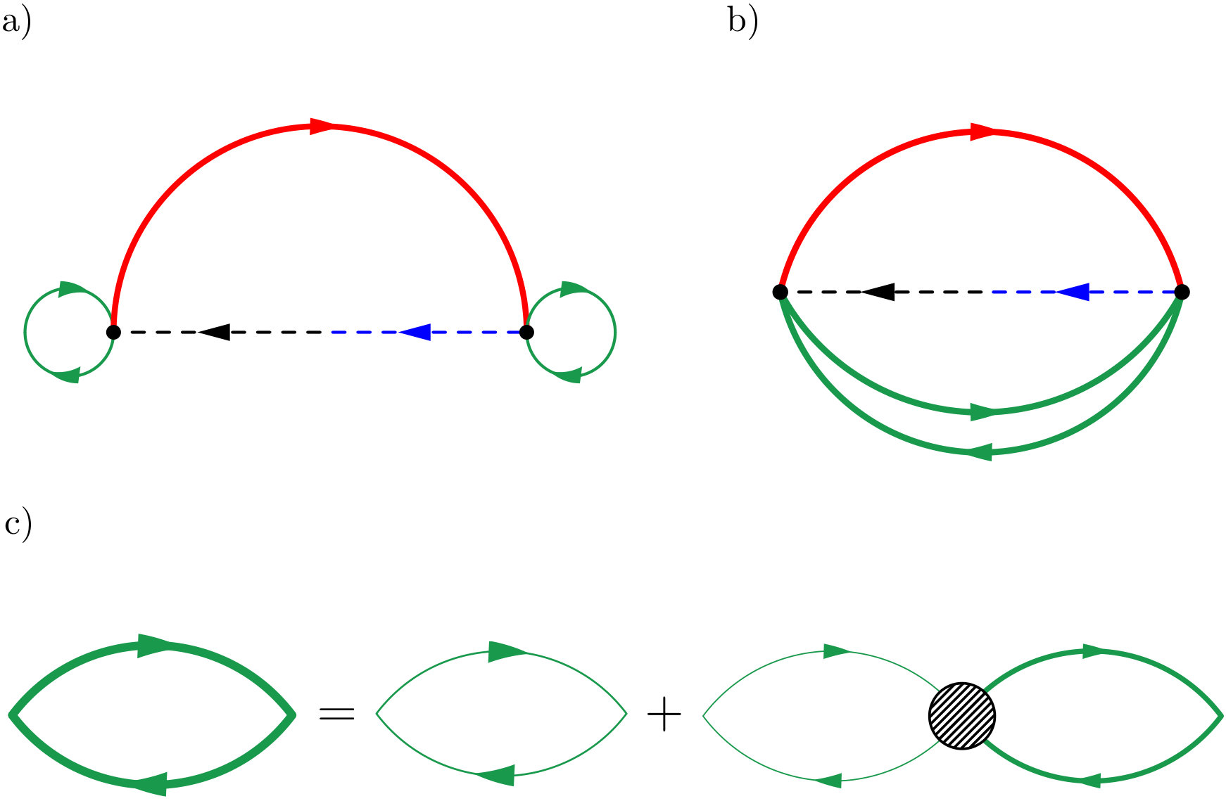 Figure 1
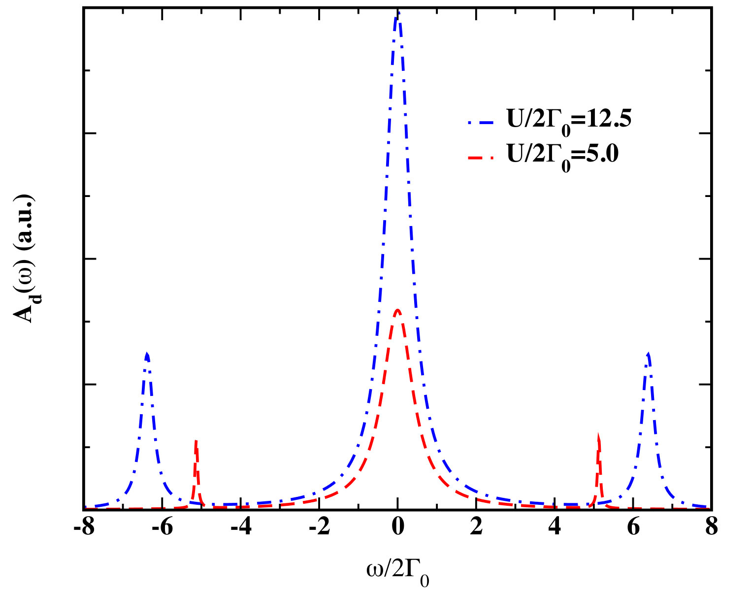 Figure 2
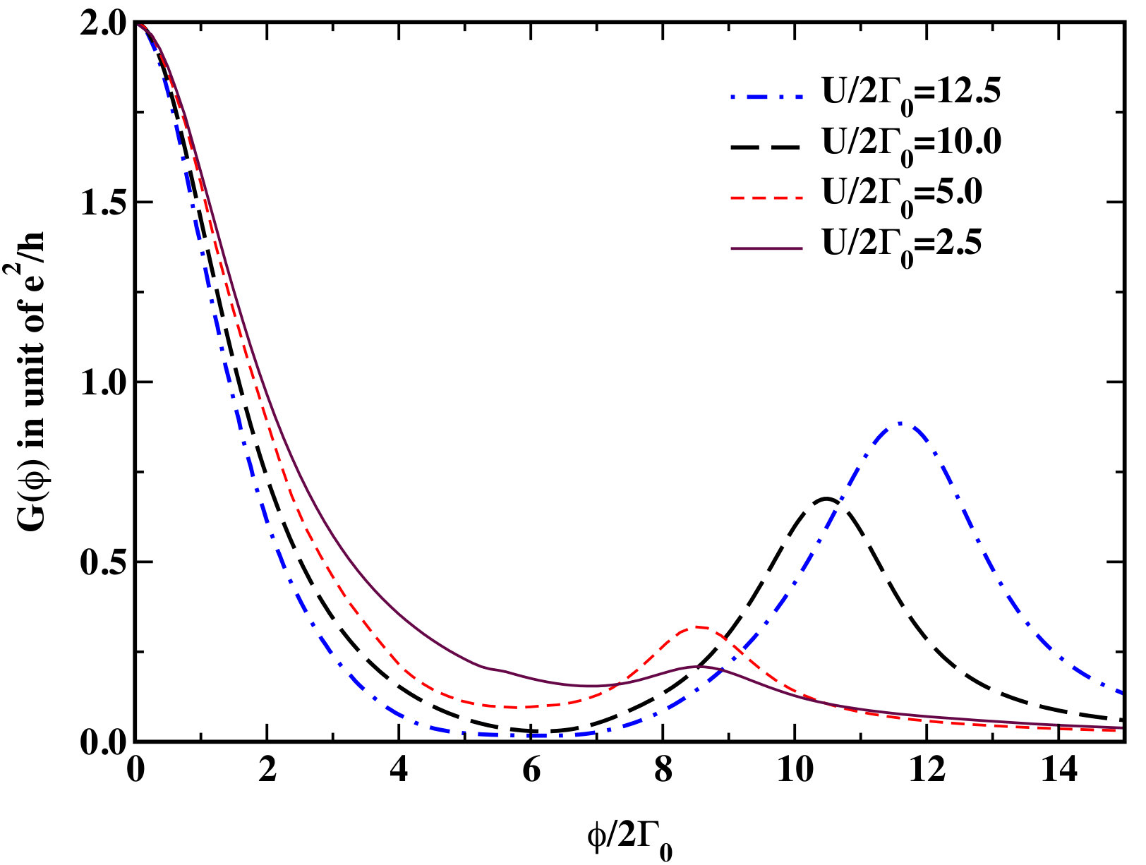 Figure 3
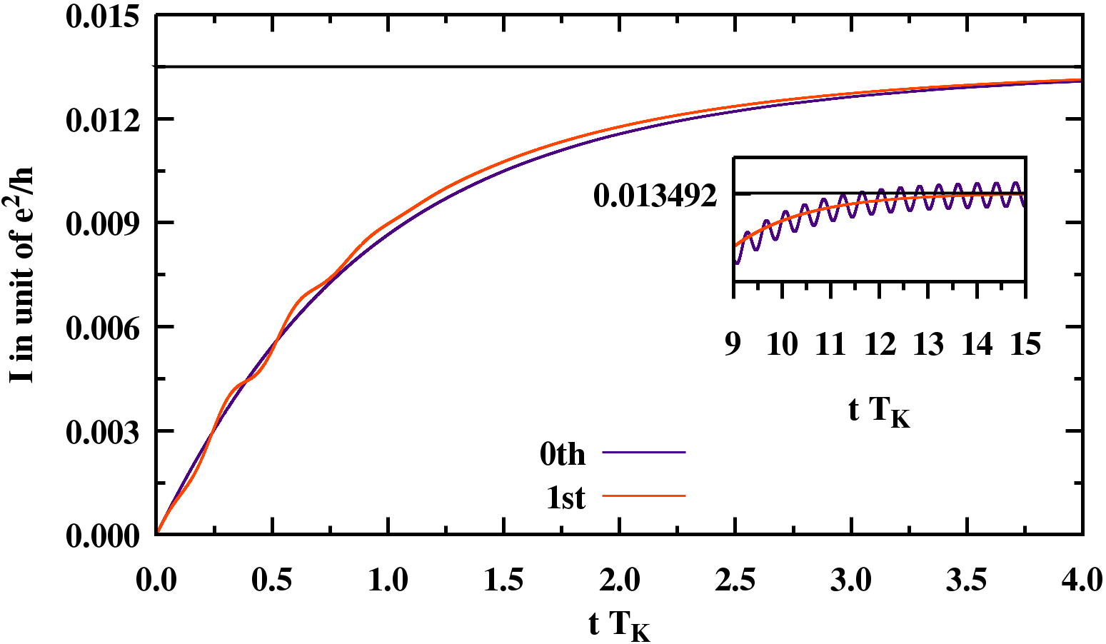 Figure 4
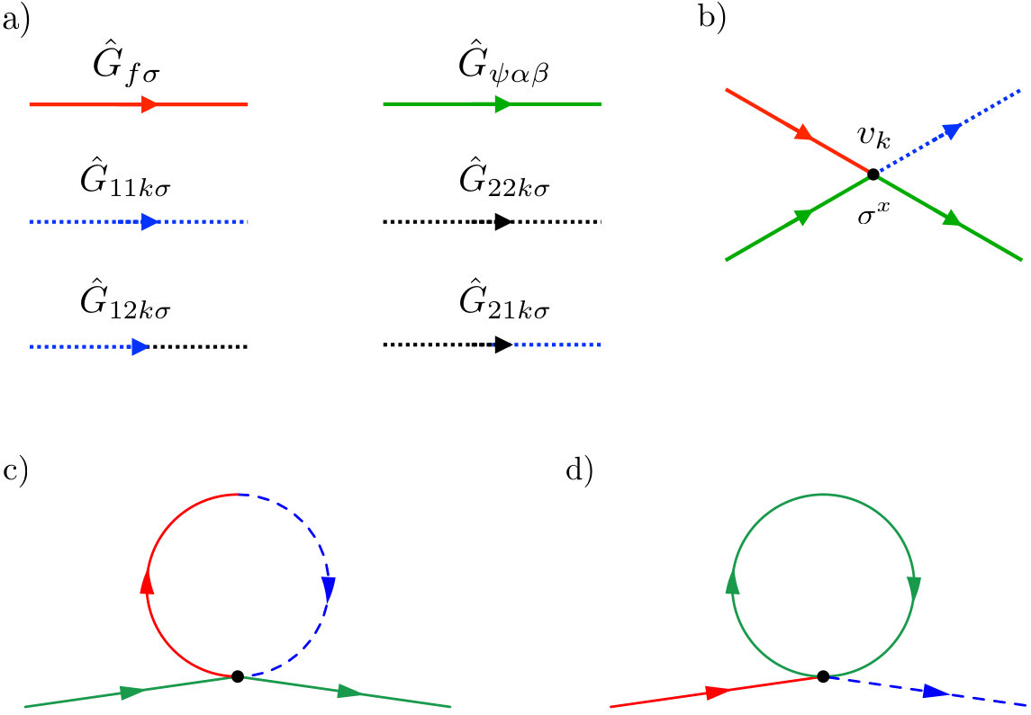 Figure 5
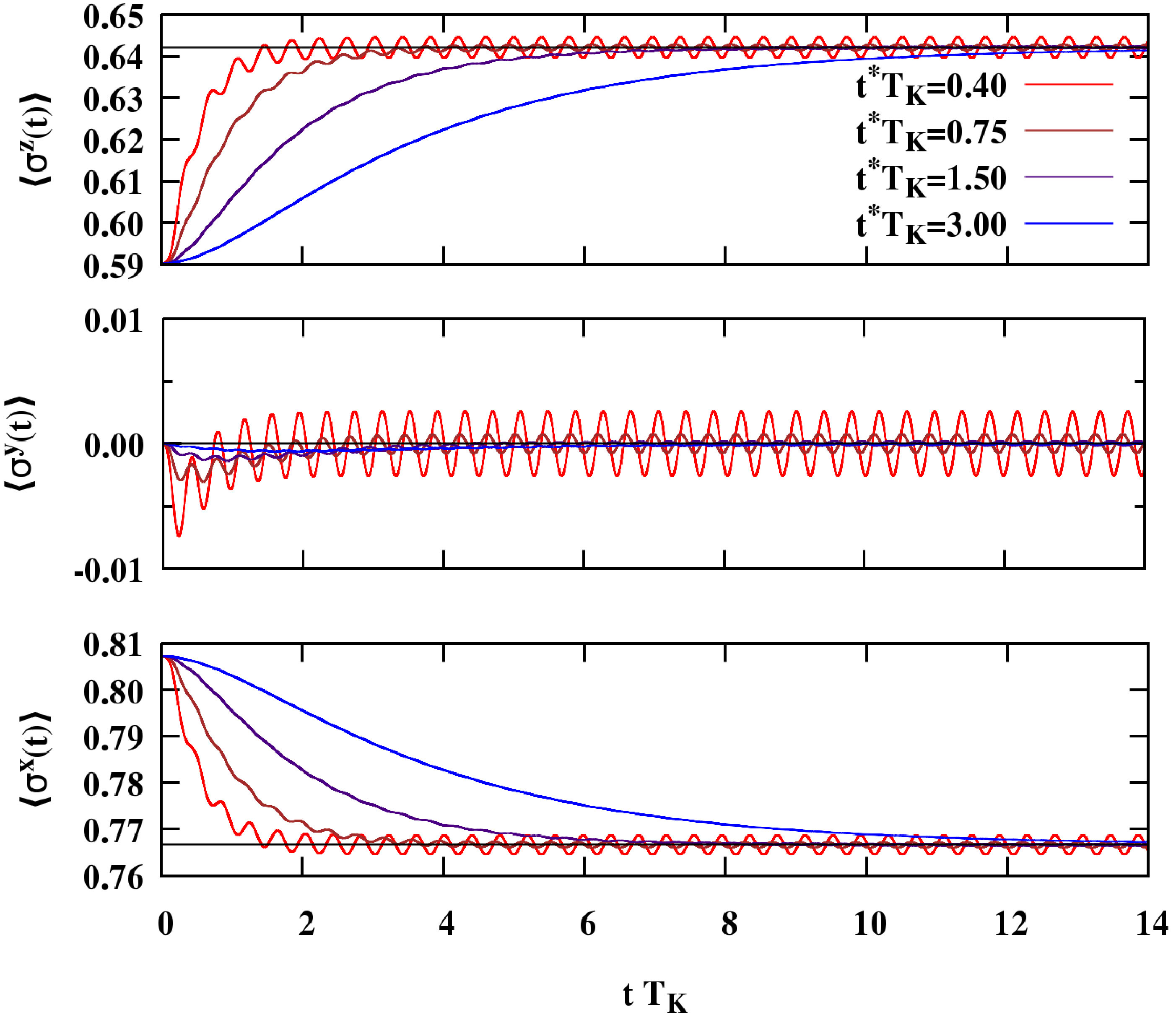 Figure 6
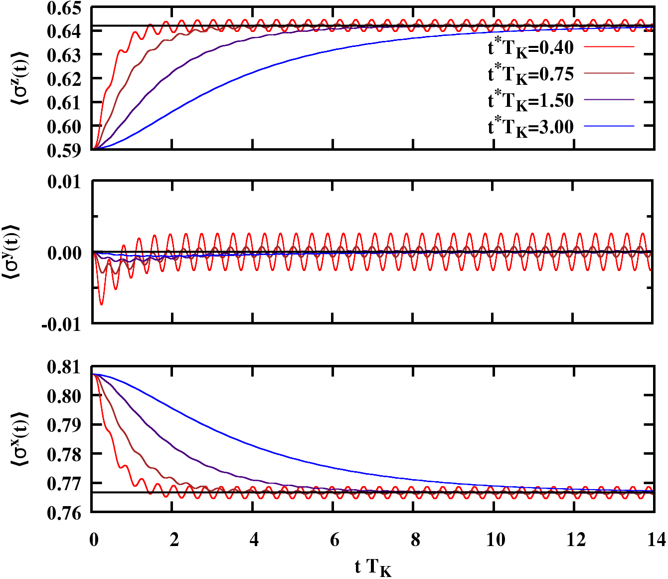 Figure 7
Peer Reviews
No public reviews on file for this paper yet. If you reviewed it on a platform where reviews are public (OpenReview, ICLR, NeurIPS, ICML), you can paste yours below so the community can read it here.
Videos
No videos yet. Explain this paper in a talk, walkthrough, or lecture? Add one.
Transport through a magnetic impurity: a slave-spin approach
Daniele Guerci
International School for Advanced Studies (SISSA), Via Bonomea 265, I-34136 Trieste, Italy
(March 15, 2024)
Abstract
We study transport across a magnetic impurity by means of a recently developed slave-spin technique that does not require any constraint. Within a conserving mean-field approximation we find a conductance that displays both the known zero-bias anomaly but also the expected peak at bias of order . We extend the slave-spin mean-field approximation to study the out of equilibrium transient evolution of a quantum dot. We apply the method to investigate the time-evolution of a quantum dot induced by a time-dependent electrochemical potential applied to the contacts. Similarly to the time-dependent Gutzwiller approximation, the mean-field slave-spin dynamics is able to capture dissipation in the leads, so that a steady-state is reached after a characteristic relaxation time.
I Introduction
Originally observed in magnetic alloysHewson (1993), the Kondo effectKondo (1964); Anderson (1970), maybe the simplest collective phenomena due to strong correlations, is now routinely realized in magnetic nanocontacts, either by real magnetic atoms and moleculesStefan et al. (2014); Martínez-Blanco et al. (2015); Pan et al. (2015) or artificial onesKastner (1993); Ashoori (1996), e.g. quantum dots, and reveals itself by the so-called zero-bias anomalyGoldhaber-Gordon et al. (1998); Cronenwett et al. (1998); Glazman and Raikh (1988); Ng and Lee (1988). It arises by the coupling between a single magnetic atom, such as cobalt, and the conduction electrons of an otherwise non-magnetic metal. Such an impurity typically behaves like a local moment that, due to spin exchange, forms a many-body spin singlet state with the itinerant electrons.
Unlike magnetic alloys, nanoscale Kondo systems can be driven out of equilibrium by applying charge or spin bias voltages across the devicesKobayashi et al. (2010). In such a nonequilibrium situation, the interplay between the time dynamics and strong correlation effects makes the theoretical description extremely challenging. To address this problem many innovative approaches has been developed, such as time-dependent numerical renormalization groupAnders and Schiller (2005, 2006); Anders (2008), real time Monte CarloWerner et al. (2009); Schiró and Fabrizio (2009), time-dependent density-matrix renormalization groupWhite and Feiguin (2004); Schmitteckert (2004); Boulat et al. (2008), flow equation methodsKehrein (2005); Fritsch and Kehrein (2010); Tomaras and Kehrein (2011), perturbative renormalization groupNordlander et al. (1999); Kaminski et al. (2000); Rosch et al. (2003); Metzner et al. (2012); Schoeller (2009), time-dependent variational approachesAshida et al. (2018); Lanatà and Strand (2012), slave-particle techniquesCitro and Romeo (2016); Ludovico and Capone (2018); Dong and Lei (2001); Raimondi and Schwab (1999) and exact approachesMehta and Andrei (2006); Bolech and Shah (2016). Despite the rich variety of methods, they often become numerically costly at long times, which limit their application to the short times evolution of simple models. However, some of themLanatà and Strand (2012); Citro and Romeo (2016), even if less accurate, are semianalytical methods able to study the full out of equilibrium evolution of realistic systems.
To the latter class of approaches belongs the nonequilibrium slave-spin technique for magnetic impurities we present in this paper. By means of a recently developed slave-spin techniqueGuerci and Fabrizio (2017), we map without any constraint a single -orbital Anderson impurity model (AIM), characterized by a particle-hole symmetric hybridization with the contacts, onto a resonant level model coupled to a single quantum pseudospin. In this suitable representation, a simple self-consistent Hartree-Fock calculation is able to reproduce qualitatively the differential conductance of a single-orbital magnetic impurity both in the small and large bias regimes. Moreover, the slave-spin technique allows to study the full time evolution of magnetic impurities coupled with metallic leads under a nonequilibrium protocol.
The plan of the paper is as follows: we first introduce the AIM to describe a single-orbital magnetic impurity coupled with metallic contacts in section II. We then present in section II.1 our slave-spin mapping, which allows to compute time-dependent average values without any constraint, details are given in section II.2. In section III we present the mean-field approximation for the out of equilibrium dynamics of a single-orbital magnetic impurity. Then, by assuming that the system relaxes after an initial transient, we present, in section IV, the mean-field approximation for the nonequilibrium steady-state regime. To highlight the importance of the approach presented in this work, section V is devoted to the application of the method to transport in magnetic impurities coupled with metallic contacts. In particular, in section V.1, we consider the nonequilibrium steady-state induced by applying a constant voltage to the contacts. Furthermore, in section V.2 we compute within a self-consistent approximation scheme the steady-state differential conductance. Finally, section V.3 is devoted to the analysis of the out of equilibrium evolution induced by a time-dependent voltage applied to the metallic contacts. Technical points of the calculations are given in appendices A, B and C at the end of the paper.
II The model
We model a single-orbital magnetic impurity coupled to left () and right () contacts in terms of an AIM
[TABLE]
where the first term corresponds to an interacting impurity
[TABLE]
where is the annihilation operator of an electron state on the impurity, the corresponding density, and . In Hamiltonian (2) denotes the charging energy, the gate potential and the Zeeman field applied on the dot. The non-interacting leads are represented by a free electron gas with half-bandwidth
[TABLE]
where is the elettrochemical potential that fixes the number of electrons in each contact, .
Finally, the tunneling coupling between the leads and the central region is represented by:
[TABLE]
where is a time-dependent tunneling amplitude, and is the number of states. In this article we limit the analysis to the symmetric case where . Furthermore, we assume a particle-hole symmetric bath, i.e. for any there exist a such that and:
[TABLE]
where
[TABLE]
Under a spin- particle-hole transformation
[TABLE]
the Hamiltonian (1) parameters change as follows,
[TABLE]
where upper and lower signs refer to the action of and , respectively. The particle-hole transformation (6) has been defined by mixing and contacts to leave the electrochemical potential (3) invariant.
To study transport across the impurity is convenient to perform the Glazman-Raikh rotation Glazman and Raikh (1988):
[TABLE]
We notice that the anti-symmetric combination of the electron states in the leads is fully decoupled from the impurity, while the symmetric combination remains coupled to , see Eq. (4). Thus, the Kondo screening involves only the variables. On the other hand, the current operator is expressed in terms of only:
[TABLE]
where the current operator, defined as and , is invariant under the particle-hole transformation (6).
II.1 The slave-spin representation
In the local magnetic regime, when is by far the largest energy scale, charge fluctuations are well-separated in energy from spin ones. However, Hamiltonian (1) lacks a clear separation between charge and spin degrees of freedom that is desirable in the magnetic moment regime. To disentangle low and high energy sectors we enlarge the original Hilbert space by adding a single quantum pseudospin variable :
[TABLE]
where and . Therefore, we encode valence fluctuations, measured by the operator:
[TABLE]
in by imposing the local constraint that filters the physical subspace out from the enlarged Hilbert space :
[TABLE]
Consequently, the eigenstates of refer to the presence or the absence of a local magnetic moment in the impurity site. In addition, we introduce two auxiliary fermionic operators that annihilate a pseudofermion state on the impurity. The precise relation between the original electrons and the auxiliary degrees of freedom is given by:
[TABLE]
ensuring the anticommutation relations . In the physical subspace, which is selected by the projector
[TABLE]
the original model (1) is equivalent to:
[TABLE]
where remains unalterated, is obtained by replacing with in Eq. (4), while the dot Hamiltonian is:
[TABLE]
Thus, the original Anderson impurity model is mapped into a resonant level model coupled to the pseudospin operator in the presence of a transverse field along the component. We observe that the Hamiltonian possesses a local gauge symmetry generated by the parity transformation . Therefore, the quantum dynamics, induced by the operator , couples the singly occupied impurity configuration with and does not mix physical and unphysical subspaces.
Finally, we notice that in the physical subspace the current operator reads:
[TABLE]
where , defined in Eq. (9), contains pseudofermion operators.
Remarkably, the time-dependent evolution of the AIM, Eq. (1), can be obtained from the auxiliary model in Eq. (12) without any constraint on the enlarged Hilbert space. The proof of this equivalence follows the same steps of the equilibrium case, see Ref. Guerci and Fabrizio (2017).However, we consider valuable to show, in the next section, the possibility to remove the constraint in the time-dependent average value of the charge current, defined in Eq. (9).
II.2 Fate of the constraint in the dynamics
Without losing generality, we assume the model in Eq. (12) prepared at time in thermal equilibrium at temperature :
[TABLE]
where and the impurity is decoupled from the contacts . For we let the system evolve by suddenly changing the coupling bewteen the bridging region and the leads: . We note that the initial distribution may include a chemical potential bias between and contacts. The average current flowing across the dot (9) is defined as:
[TABLE]
where is the unitary time evolution operator. Since the trace is invariant under similarity transformations and , Eq. (7) implies:
[TABLE]
and
[TABLE]
Within the slave-spin representation the initial equilibrium distribution is described by
[TABLE]
and the average value of the current reads
[TABLE]
where the trace is on the enlarged Hilbert space, , defined in Eq. (11), is the projector in the physical subspace and is the time evolution operator generated by . In the slave-spin representation (12) the role of the p-h symmetry transformation is simply played by , so
[TABLE]
Eq. (15) implies:
[TABLE]
Since , it readily follows that:
[TABLE]
where we have used the equivalence . Eq. (16) states that the time-dependent average value of the current flowing across the impurity (1) can be computed in the slave-spin representation (12) without any constraint.
Following the same line of reasoning, previous result extends to any time-dependent average of physical observables and holds for any nonequilibrium protocol. Thus, we conclude that the out of equilibrium evolution of the original model (1) can be obtained within the slave-spin representation (12) without projecting out unphysical configurations introduced by the mapping (10).
III Time-dependent Mean-field equations
In this section we present the mean-field approximation to describe the out of equilibrium evolution of a driven magnetic impurity. The dynamics of the AIM (1) is governed by the time-dependent Schrödinger equation:
[TABLE]
where at the system is prepared in the ground state configuration of the initial Hamiltonian Eq. (12).
The mean-field approach consists in approximatingGuerci and Fabrizio (2017) the time-dependent wave function with a factorized one product of a fermionic part times a spin one :
[TABLE]
We notice that the previous approximation is appropriate in the local moment regime, i.e. , where the two subsystems are characterized by well-separated energy scales. This is indeed the regime we consider hereafter.
The dynamics of the interacting model (17) is, thus, reduced to the evolution of a spin degree of freedom:
[TABLE]
under a self-consistent time-dependent magnetic field:
[TABLE]
Eq.(19) is coupled with the Schrödinger Eq. for the Slater determinant :
[TABLE]
where the effective fermionic Hamiltonian is
[TABLE]
and . For a given initial configuration, , Eqs. (19) and (20) allow to study the dynamics of the original correlated model in terms of the evolution of a spin coupled with a time-dependent Resonant level model.
As observed in section II.2, we emphasize that the nonequilibrium evolution of the Hamiltonian (1) can be obtained by the slave-spin representation without any need of local constraints that project out unphsyical configurations introduced by the mapping (10). The advantages, respect to other slave-particles approachesCitro and Romeo (2016); Raimondi and Schwab (1999), are twofold. On one side, we reduce the number of dynamical equations. On the other side, we avoid the mean-field mixing of unphysical and physical subspaces.
The dynamical Eqs. (19) and (20) are equivalent to the ones obtained by applying the time-dependent Gutzwiller approximation (t-GA) Schiró and Fabrizio (2010) to the AIM Lanatà and Strand (2012). In this regard, the evolution of the time-dependent Gutzwiller parameters resemble the dynamics of the spin variable, while the bath and the pseudofermion degrees of freedom evolve under a time-dependent self-consistent Hamiltonian (21).
For large time, namely after the transient, we assume that, due to the coupling with infinite contacts, the solution of Eqs. (19) and (20) thermalizes to a steady-state. In order to describe the asymptotic regime we develop, in the next section, the nonequilibrium stationary mean-field approach.
IV Mean-field for the nonequilibrium steady-state
In this section we discuss the mean-field approximation in the nonequilibrium steady-state.
Without losing generality, we shall assume that at the contacts are disconnected to the dot but in the presence of a finite bias, so that their distribution functions read:
[TABLE]
where is the voltage difference applied to the contacts and is the Fermi-Dirac distribution function. Once the tunneling amplitude (4) is turned on, a time-dependent current starts to flow across the junction accordingly to Eqs. (19) and (20). For large time, namely after the transient, we assume that the system described by the ground-state reaches a stationary state
[TABLE]
characterized by a constant current. We observe that Eq. (23) is a justified assumption. Indeed, as presented in section V.3, the slave-spin mean-field evolution predicts, for large time, the existence of a steady-state due to the coupling of the dot with infinite contacts.
Following the same reasoning of section III, the stationary mean-field approach consists in approximatingGuerci and Fabrizio (2017) the ground-state wave function (23) with a factorized one:
[TABLE]
where is the fermionic part and the spin one. At stationarity, the pseudospin degree of freedom is controlled by the Hamiltonian:
[TABLE]
where and
[TABLE]
are expectation values in the fermionic steady-state wave function. The ground-state of (25) is identified by:
[TABLE]
where for convenience we have introduced the self-consistent magnetic field:
[TABLE]
The fermionic problem is, thus, reduced to find the steady-state ground-state of the quantum Hamiltonian
[TABLE]
where is introduced in the aforementioned unitary transformation (8) and
[TABLE]
Since we deal with a nonequilibrium situation we work in the framework of the Keldysh technique, as employed in the literature Rammer (2007); Haug and Jauho (1996); Arseev (2015). Eq. (26) requires the evaluation of the lesser Green’s function , which, by means of the Dyson’s Eq., can be expressed in terms of the dressed Green’s function of the pseudofermions and the free Green’s function of the contacts. Instead, Eq. (27) can be expressed in terms of the pseudofermions Green’s function only. By performing straightforward calculations, that are summarized in appendix A, we obtain:
[TABLE]
where the nonequilibrium distribution on the impurity is and the pseudofermion spectral function reads
[TABLE]
Within the mean-field approximation, the pseudofermions self-energy is given by:
[TABLE]
where the factor of 2 counts the presence of two different leads, while the hybridization function is defined in Eq. (5).
Given the spectral properties of the contacts, i.e. , Eqs. (31) and (32) give an analytic expressions for the effective magnetic field , which depends on the steady-state average . Therefore, we close the set of mean-field equations and the steady-state variational ground-state is obtained by solving:
[TABLE]
that corresponds to a root-finding problem in a single angular variable .
Before concluding the section, we observe that the nonequilibrium steady-state self-consistent Eq. (33) is equivalent to the one obtained with the out of equilibrium Gutzwiller approach for quantum dotsLanatà (2010). However, in comparison with the latter approach, the slave-spin method has the advantage of allowing one to use the machinery of quantum field theory, i.e. Wick’s theorem, to improve mean-field results by including fluctuations.
V Application to transport thorugh a magnetic impurity
The last section of this work is devoted to the application of the method, developed in sections III and IV, to study the nonequilibrium dynamics of a magnetic impurity coupled with metallic contacts. To highlight the importance of our formulation here we consider the simple case , and we take the wide-band limit (WBL). Moreover, we will firstly analyze the steady-state regime by computing the nonequilibrium ground-state and the differential conductance as a function of the voltage applied to the contacts. Then, we will study the out of equilibrium evolution induced by a slowly varying time-dependent voltage.
V.1 The steady-state solution in the wide band limit
Initially, we assume the dot disconnected by the leads, which are prepared at two different chemical potential , so that their initial distribution function is described by Eq. (22). Once the tunneling amplitude is turned on, after the initial transient, the steady-state Hamiltonian, that describes the quantum pseudospin degree of freedom, is given by:
[TABLE]
In the wide-band limit, where , the electron self-energy reduces to
[TABLE]
and we readily find that
[TABLE]
where is the renormalized hybridization amplitude . The steady-state variational ground-state is obtained by solving the self-consistent equation:
[TABLE]
For large , and , the solution of the self-consistent Eq. (36) for reads:
[TABLE]
where
[TABLE]
is the same as in slave-boson mean-field theory, and can be associated with the Kondo temperature , though overestimated respect its actual value Baruselli and Fabrizio (2012). As shown in Eq. (37) the effect of an external voltage , within mean-field approximation, is to reduce the equilibrium value of the renormalized hybridization . Moreover, the mean-field steady-state breaks spontaneously the gauge symmetry by choosing one of the two degenerate minima , as already observed in the equilibrium case Ref.Baruselli and Fabrizio (2012).
At the steady-state variational minimum we can compute the average value of the current:
[TABLE]
that involves the evaluation of the two-particle correlation function . In a consistent approximation scheme the self-energy corrections have to be included in two-particle correlation functions through the Bethe-Salpeter equation. In the next section, by means of the Abrikosov representationAbrikosov (1965) of the pseudospin variable , we readily compute the average value of the current (38) consistently with the mean-field approximation (24).
V.2 The steady-state current within a self-consistent mean-field approximation
To perform a self-consistent calculation of the current, Eq. (38), we introduce a couple of fermionic operators corresponding to the pseudospin operator according to the formulaAbrikosov (1965):
[TABLE]
where the upper index denotes the Pauli matrices, while . The fermion substitution Eq. (39) introduces two additional configurations and to the two dimensional Hilbert space of the -matrices, which is composed by and . However, in the case of spin the unphysical configurations are automatically excluded since physical quantities involve only averages of products of , which have the property of giving zero when acting on the non-physical states or .
In this representation, the hybridization term in Eq. (4) becomes the four-leg fermionic interaction vertex depicted in Fig. 1 b). The Hartree-Fock approximation corresponds to the mean-field decoupling presented in section IV, and is described by the self-energy diagrams in Figs. 1 c) and d). The average value of the current reads:
[TABLE]
and implies the evaluation of the two-particle correlation function . Therefore, consistently with the slave-spin mean-field decoupling the current is made up of two contributions, Figs. 2 a) and b):
[TABLE]
where the former, , involves only the low-energy pseudofermion degree of freedom, and can be obtained by straightforward calculations summarized in appendix A. Here, we report the final result in the WBL:
[TABLE]
where is the elementary charge and the Planck’s constant.
Instead, the latter term in Eq. (40) takes into account the contribution of valence fluctuations and can be expressed as
[TABLE]
where the kernel is given by:
[TABLE]
where is the fermion spin-correlation function, for more details we refer to appendix B. Consistently with the Hartree-Fock approximation satisfies the Dyson’s Eq. in Fig. 2 c), whose solution for the retarded component reads:
[TABLE]
and the lesser component:
[TABLE]
where and . The self-energies appearing in Eqs. (43) and (44) are obtained by contracting the four-leg vertex in Fig. 1 b), details can be found in appendix B. Specifically, the self-energy allows to reconstruct incoherent side bands characterized by a width of the order of the bare hybridization and centered around as shown in Fig. 4.
Numerical integration of Eq. (42) permits to compute the differential conductance
[TABLE]
which is shown in Fig. 3. We observe two distinct contributions: (i) the well-known zero-bias anomaly which derives from the Kondo peak at the Fermi level and controls the low-bias behavior and (ii) an incoherent one, which mainly contributes to the large bias features of the conductance.
To compare our result for with the universal behavior of the conductance in the Kondo regime, obtained with renormalization group approach in Refs.Pustilnik and Glazman (2004); Sela et al. (2006), we expand around obtaining:
[TABLE]
In agreement with our self-consistent Hartree-Fock approximation, Eq.(45) reproduces exactly the contribution given by the phase shift, while neglects the contribution from the residual scattering among low-energy quasiparticlesNozières (1974). We believe that, in the slave-spin representation, the latter contribution comes from vertex corrections, that are not included in our perturbative calculation.
V.3 Adiabatic dynamic induced by a time-dependent voltage
Physically, applying a time-dependent voltage between the source and the drain contacts means that the single-particle energies become time-dependent: (here label refers to the left or right lead) Jauho et al. (1994). Starting, at , from an equilibrium configuration characterized by () and a finite tunneling amplitude , we consider the evolution induced by a time-dependent electrochemical potential:
[TABLE]
where is the characteristic time scale of the external perturbation, is the asymptotic value of the voltage and is the Heaviside step function such that for . Here we consider the WBL analogously to the steady-state analysis. The dynamic of the pseudospin variable is:
[TABLE]
where the time-dependent average value of the hybridization is given by:
[TABLE]
In this case (48), the normal product is substituted with , while and are the Wigner transform of the lesser component of the self-energy and the advanced Green’s function of the pseudofermions, for more details we refer to appendix C.
In the following, we consider an external perturbation , which is a slowly varying function of time compared to the characteristic scales of the equilibrium state, i.e. . Therefore, we can assume that the temporal inhomogeneity is weak and only lowest-order terms in the variation are kept, the so-called gradient expansion Rammer (2007); Haug and Jauho (1996).
To the first-order in the temporal variation we have:
[TABLE]
where , more details can be found in Appendix C.
The evolution of the pseudospin variable induced within the zeroth order in the gradient expansion Eq. (49) is displayed in Fig. 5. In the limit of we observe, as expected, the quasistatic dynamic, i.e. the system stays in equilibrium at all times and follows the change of adiabatically. However, for any smaller value of the dynamics is characterized by persistent oscillations, that become, eventually, centered around the steady-state result represented by the solid black line.
Remarkably, first-order correction, given by the latter term in Eq. (49), introduces a relaxation mechanism and the dynamic converges to the expected stationary regime. This is shown in Fig. 6, where we compare the time-dependent average value of the current obtained within the zeroth and first order in the gradient expansion.
VI Conclusions
We have shown that the out of equilibrium evolution of a single-orbital AIM (1) can be calculated in the slave-spin representation (12) without any constraint on the enlarged Hilbert space. The advantages of the new representation are twofold. On one side, we disentangle charge and spin degrees of freedom. On the other side, we avoid the mean-field mixing of unphysical and physical subspaces, that affects the time evolution of other slave-particle techniques. In the steady-state regime the self-consistent Hartree-Fock decoupling is able to predict properties of the model even deep inside the large- Kondo regime, specifically, the conductance shows both the known zero-bias anomaly but also the expected peak at bias of order . Furthermore, we have extended the slave-spin approach to study the transient dynamic of a driven magnetic impurity. By means of a time-dependent Hartree-Fock calculation, in the adiabatic regime, we prove that, at first-order in the gradient expansion, the current relaxes to the steady state value after an initial transient.
Finally, we mention that the technique we have proposed can be applied to study the out of equilibrium dynamics of multi-orbitals magnetic impurities by using the generalized mapping presented in Ref.Guerci and Fabrizio (2017).
Acknowledgments
I am grateful to Michele Fabrizio for insightful discussions that allowed me to clarify several important points related to this work and for a careful reading of this manuscript. Furthermore, I thank Roberto Raimondi, Francesco Grandi, Massimo Capone, Laura Fanfarillo, Valentina Brosco, Maria Florencia Ludovico and Adriano Amaricci for constructive discussions on the manuscript. We acknowledge support from the H2020 Framework Programme under ERC Advanced Grant No. 692670 FIRSTORM.
Appendix A The effective Resonant level model in the steady-state regime
In this section we derive analytic expressions for the hybridization Eq. (26) and the current Eq. (41). Morover, we compute the Keldysh’s components of the and fermion Green’s function within Hartree-Fock approximation.
pseudofermion Green’s function
The unperturbed retarded and advanced Green’s functions of the contacts are
[TABLE]
and
[TABLE]
where we have already performed the rotation in Eq. (8). In terms of the matrix representation
[TABLE]
the Dyson’s equation for the pseudofermion Green’s function on the Keldysh’s contour is:
[TABLE]
where is the dressed Green’s function and the unperturbed one. In Eq. (51) we use a notation where the product is interpreted as a matrix product in the internal variables (time and Keldysh’s indeces). In the stationary regime the time translational invariance is restored, thus, by taking the Fourier transform of Eq. (51) we obtain:
[TABLE]
and
[TABLE]
Within mean-field approximation the self-energy of the reads:
[TABLE]
and
[TABLE]
Expectation values
The average occupation on the quantum dot (32) follows from Eqs. (53) and (54). The average value of the hybridization (26) involves the lesser component of the mixed Green’s function:
[TABLE]
Thus,
[TABLE]
By using Eqs. (52), (53) and (54) we readily obtain Eq. (31) reported in the main text. Finally, we briefly derive the expression for the low-energy contribution to the current average value Eq. (41). In this case the mixed Green’s function involved is and its Dyson’s equation reads:
[TABLE]
The average value of the current is:
[TABLE]
where
[TABLE]
In the WBL Eq. (57) gives Eq. (41).
fermion Green’s function
The Dyson’s equation for the fermion reads:
[TABLE]
where the Hartee-Fock self-energy, depicted in Fig. 1 c) is:
[TABLE]
In Eq. (58) we are using the same notation introduced in Eq. (51), where the hat refers to the matrix structure (50). By performing straightforward calculations we obtain:
[TABLE]
where denotes the identity and the remaining Pauli matrices, while and
[TABLE]
with and solution of Eq. (33). Finally, we report the lesser component:
[TABLE]
where and
[TABLE]
Appendix B RPA corrections to the spin correlation function
In this section, we compute the RPA correction to the mode, which describes valence fluctuations on the impurity site. In terms of the fermionic representation introduced in Eq. (39) the bare propagator reads:
[TABLE]
where is the Hartree-Fock fermion Green’s function in Eq. (58). As shown in Fig. 2 c) the Dyson’s equation reads:
[TABLE]
where we adopt the notation introduced in Eq. (50). At RPA level the bosonic self-energy reads:
[TABLE]
with:
[TABLE]
where , and is the hybridization operator in Eq. (4). Within the WBL, introduced in Eq. (34), the evaluation of the bosonic self-energy (59) is considerably simplified. We find:
[TABLE]
and
[TABLE]
Appendix C Transient dynamics of the effective Resonant level model
The dynamics of the spin degree of freedom is influenced by the time-dependent expectation value of the hybridization Eq. (48). By assuming a slowly varying electrochemical potential (46), we compute Eq. (48) to the first-order in the gradient expansion Eq. (49). To this aim we define the Wigner transform of the pseudofermion Green’s function:
[TABLE]
which satisfies the Dyson’s equation:
[TABLE]
where denotes the Moyal product introduced in the main text. The solution of the Dyson’s equation up to first-order is:
[TABLE]
where in the WBL the time-dependent self-energy is . Instead, the lesser self-energy is given by:
[TABLE]
where and the nonequilibrium distribution reads
[TABLE]
In the last passage of Eq. (60), we assume that the dependence of on the relative time is negligible.
In the following, we report the zeroth and first-order contributions to the gradient expansion of .
Zeroth order
The zeroth order contribution, first term in Eq. (49), reads:
[TABLE]
where the pseudofermion time-dependent spectral function is
[TABLE]
with .
First order
The first order correction to the quasistatic approximation is the second term of Eq. (49), which reads:
[TABLE]
After straightforward calculations we obtain
[TABLE]
Since the latter contribution modifies the Heisenberg equation (47) by introducing a finite relaxation in the evolution of the component.
The reference list from the paper itself. Each links out to its DOI / PubMed record.
- 1Hewson (1993) A. C. Hewson, The Kondo Problem to Heavy Fermions , Cambridge Studies in Magnetism (Cambridge University Press, 1993).
- 2Kondo (1964) J. Kondo, Progress of Theoretical Physics 32 , 37 (1964), URL http://dx.doi.org/10.1143/PTP.32.37 . · doi ↗
- 3Anderson (1970) P. W. Anderson, Journal of Physics C: Solid State Physics 3 , 2436 (1970), URL http://stacks.iop.org/0022-3719/3/i=12/a=008 .
- 4Stefan et al. (2014) F. Stefan, J. Martínez-Blanco, J. Yang, K. Kanisawa, and S. C. Erwin, Nature Nanotechnology 9 , 505 (2014), URL https://doi.org/10.1038/nnano.2014.129 . · doi ↗
- 5Martínez-Blanco et al. (2015) J. Martínez-Blanco, C. Nacci, S. C. Erwin, K. Kanisawa, E. Locane, M. Thomas, F. von Oppen, P. W. Brouwer, and F. Stefan, Nature Physics 11 , 640 (2015), URL https://doi.org/10.1038/nphys 3385 . · doi ↗
- 6Pan et al. (2015) Y. Pan, J. Yang, S. C. Erwin, K. Kanisawa, and S. Fölsch, Phys. Rev. Lett. 115 , 076803 (2015), URL https://link.aps.org/doi/10.1103/Phys Rev Lett.115.076803 .
- 7Kastner (1993) M. A. Kastner, Physics Today 46 , 24 (1993), URL https://doi.org/10.1063/1.881393 . · doi ↗
- 8Ashoori (1996) R. C. Ashoori, Nature 379 , 413 (1996), URL https://doi.org/10.1038/379413 a 0 . · doi ↗