Temporal dissipative solitons in time-delay feedback systems
Serhiy Yanchuk, Stefan Ruschel, Jan Sieber, Matthias Wolfrum

TL;DR
This paper develops a theoretical framework for understanding temporal dissipative solitons in systems with time-delayed feedback, including their classification, stability, and examples in laser and neural models.
Contribution
It introduces a novel theory for temporal dissipative solitons with an advanced argument and classifies their spectral properties, expanding understanding beyond spatial systems.
Findings
Derived a system with an advanced argument for TDS profile determination.
Classified TDS spectrum into interface and pseudo-continuous spectrum.
Identified destabilization mechanisms leading to delocalization and modulational instability.
Abstract
Localized states are a universal phenomenon observed in spatially distributed dissipative nonlinear systems. Known as dissipative solitons, auto-solitons, spot or pulse solutions, these states play an important role in data transmission using optical pulses, neural signal propagation, and other processes. While this phenomenon was thoroughly studied in spatially extended systems, temporally localized states are gaining attention only recently, driven primarily by applications from fiber or semiconductor lasers. Here we present a theory for temporal dissipative solitons (TDS) in systems with time-delayed feedback. In particular, we derive a system with an advanced argument, which determines the profile of the TDS. We also provide a complete classification of the spectrum of TDS into interface and pseudo-continuous spectrum. We illustrate our theory with two examples: a generic delayed…
Click any figure to enlarge with its caption.
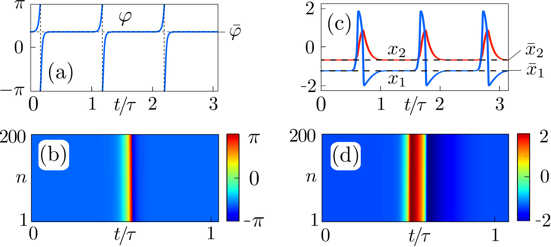 Figure 1
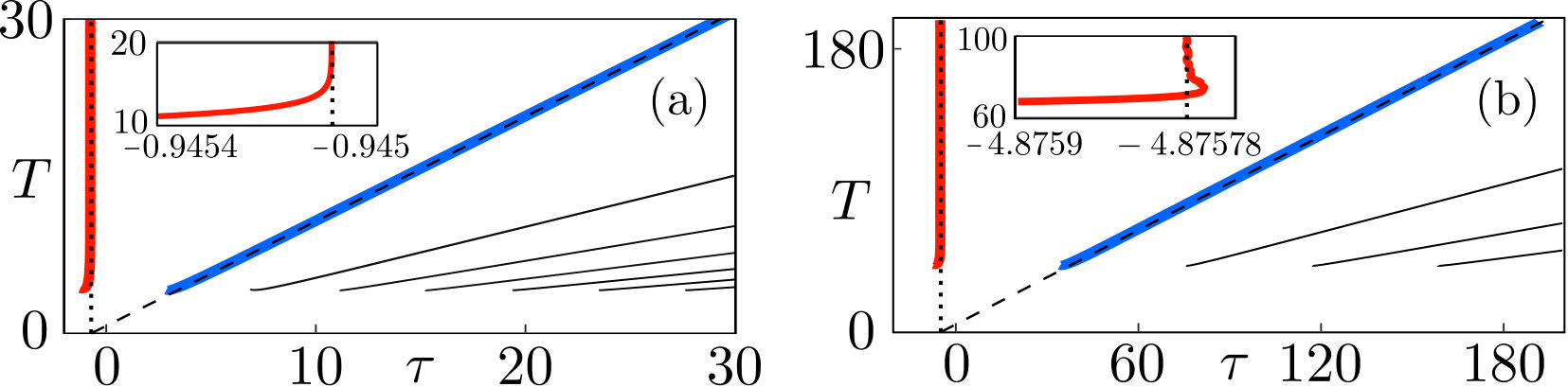 Figure 2
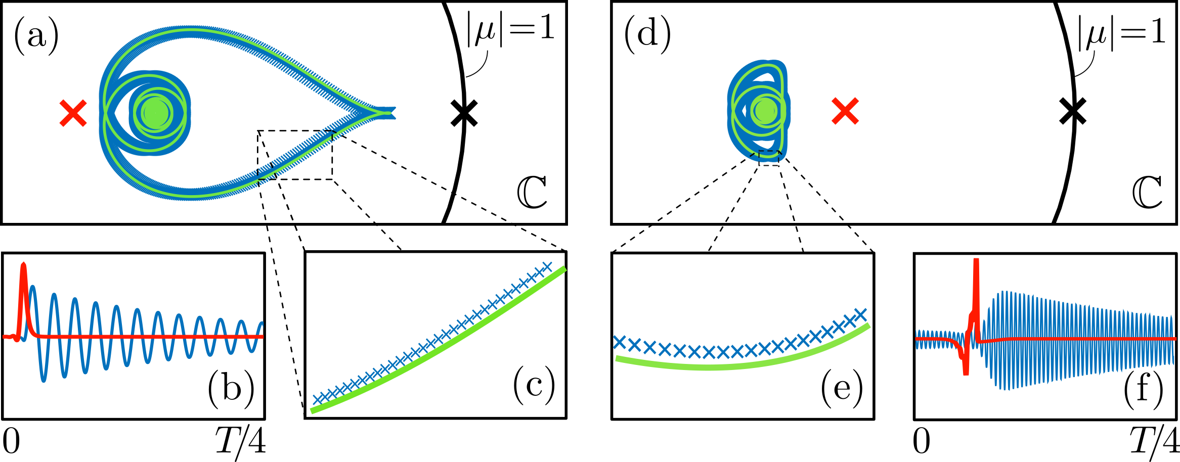 Figure 3
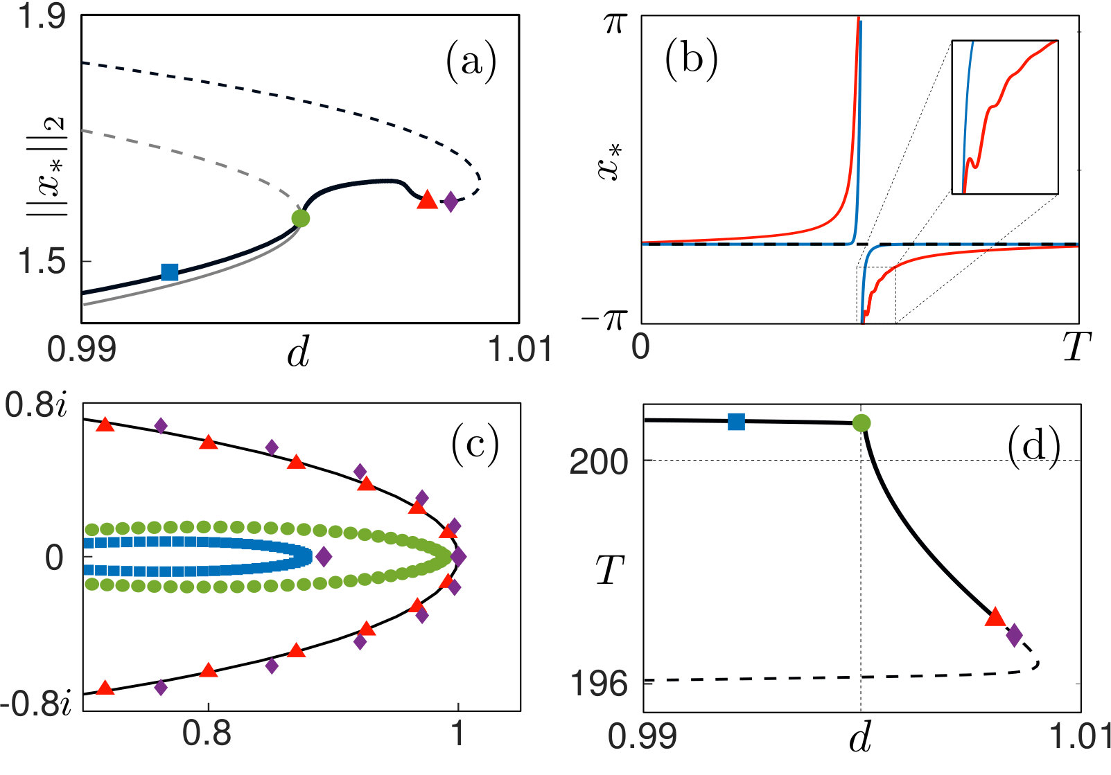 Figure 4
Peer Reviews
No public reviews on file for this paper yet. If you reviewed it on a platform where reviews are public (OpenReview, ICLR, NeurIPS, ICML), you can paste yours below so the community can read it here.
Videos
No videos yet. Explain this paper in a talk, walkthrough, or lecture? Add one.
Temporal dissipative solitons in time-delay feedback systems
Serhiy Yanchuk1, Stefan Ruschel1, Jan Sieber2, Matthias Wolfrum3
1Institute of Mathematics, Technical University of Berlin, Strasse des 17 Juni 136, 10623 Berlin, Germany
2Harrison Building, North Park Road, CEMPS University of Exeter, Exeter, EX4 4QF, UK
3Weierstrass Institute, Mohrenstrasse 39, 10117 Berlin, Germany
Abstract
Localized states are a universal phenomenon observed in spatially distributed dissipative nonlinear systems. Known as dissipative solitons, auto-solitons, spot or pulse solutions, these states play an important role in data transmission using optical pulses, neural signal propagation, and other processes. While this phenomenon was thoroughly studied in spatially extended systems, temporally localized states are gaining attention only recently, driven primarily by applications from fiber or semiconductor lasers. Here we present a theory for temporal dissipative solitons (TDS) in systems with time-delayed feedback. In particular, we derive a system with an advanced argument, which determines the profile of the TDS. We also provide a complete classification of the spectrum of TDS into interface and pseudo-continuous spectrum. We illustrate our theory with two examples: a generic delayed phase oscillator, which is a reduced model for an injected laser with feedback, and the FitzHugh-Nagumo neuron with delayed feedback. Finally, we discuss possible destabilization mechanisms of TDS and show an example where the TDS delocalizes and its pseudo-continuous spectrum develops a modulational instability.
Solitons have been known as a physical phenomenon from the early 19th century Scott Russell (1844). They are commonly associated with spatially localized states in conservative spatially extended systems, such as the Korteweg-de Vries or the nonlinear Schrödinger equation and possess remarkable properties such as preservation of localization and shape after collisions. Beyond the “classical” conservative solitons, localized states were also observed in earlier works on non-conservative chemical and physiological systems, see Purwins et al. (2010) and references therein.
Interest in localized solutions of non-conservative and non-integrable systems has grown rapidly since the early 1990s Kerner and Osipov (1994); Rosanov (2002); Akhmediev and Ankiewicz (2005, 2008); Ackemann et al. (2009); Purwins et al. (2010); Grelu and Akhmediev (2012); Parra-Rivas et al. (2013). These states have been called dissipative solitons (DS). In contrast to conservative solitons, DS are stable objects (attractors), which emerge due to a nonlinear balance between energy gain and loss Grelu and Akhmediev (2012). DS have been discovered in spatially extended systems modeled by partial differential equations in optics Kerner and Osipov (1994); Barland et al. (2002); Akhmediev and Ankiewicz (2005); Ackemann et al. (2009); Jang et al. (2013); Grelu and Akhmediev (2012); Bednyakova and Turitsyn (2015), biological systems Kerner and Osipov (1994); Heimburg and Jackson (2005); Lautrup et al. (2011); Villagran Vargas et al. (2011), plasma physics Kerner and Osipov (1994); Tur et al. (1992) and other fields Rotermund et al. (1991).
Recent experimental and theoretical results report that DS are also possible in systems with time-delayed feedback that do not include explicit spatial variables Vladimirov and Turaev (2005); Marconi et al. (2014); Marino et al. (2014); Marconi et al. (2015); Garbin et al. (2015); Romeira et al. (2016); Semenov and Maistrenko (2018); Brunner et al. (2018); Liu et al. (2018); Schelte2018 . In these systems the time delay is larger than the other timescales and the DS are temporally localized. Their natural relation to spatially localized states can be seen in a spatio-temporal representation of the dynamics of time-delayed systems as done in Giacomelli and Politi (1996); Yanchuk and Giacomelli (2017). In this representation the pulse is localized within the delay line. For example, in a ring laser this delay line corresponds physically to the ring cavity, where the optical pulse is localized Vladimirov and Turaev (2005).
Examples of systems exhibiting temporal DS (TDS) include opto-electronic setups such as mode-locked lasers with saturable absorber Vladimirov and Turaev (2005); Marconi et al. (2014); Schelte2018 , coupled broad-area semiconductor resonators Genevet et al. (2008), vertical-cavity surface-emitting lasers with delays Marconi et al. (2015), as well as neuronal models Romeira et al. (2016) or bistable systems with feedback Marino et al. (2014); Semenov and Maistrenko (2018). Although localized states have been reported mainly in one dimension, two-dimensional TDS have been found as well for a system with two feedback loops Brunner et al. (2018). In this case the lengths of the delays were significantly different. Then one can associate one spatial dimension to each delay line, thus representing the temporal dynamics using a two-dimensional spatial representation Yanchuk and Giacomelli (2014, 2015). Localized states can have different forms. For instance, they can be composed of several pulses, known as soliton molecules or bound states Marconi et al. (2015); Liu et al. (2018); Puzyrev et al. (2017). Experimental and theoretical methods to control the nucleation or cancellation of TDS have been introduced in Garbin et al. (2015); Romeira et al. (2016).
Considering the importance of TDS in systems with delayed feedback, their variety and broadness of applications, there is a need for a unifying theory describing basic properties of TDS. In this Letter, we outline such a theory for TDS with a stable equilibrium *background state *(see Fig. 1 for typical time profiles) for general systems with delayed feedback of the form
[TABLE]
where is a variable describing the state of the system, is the large feedback delay, and is a nonlinear function determining the dynamics.
We present two ingredients that enable TDS to emerge in systems (1), and introduce an equation describing the TDS time profile. Using the largeness of time delay , we describe the spectrum of Floquet multipliers of TDS. This spectrum consists of two parts. The first is the pseudo-continuous spectrum (PCS), determined entirely by (but not equal to) the spectrum of its background state. We provide an explicit expression for the PCS when the time-delayed feedback has rank 1 and a simple description for PCS computation otherwise. The second part is a point (or interface) spectrum, for which we provide an asymptotic approximation that is independent of the large delay and hence can be evaluated numerically (see Sieber et al. (2014)). The obtained results predict possible destabilization mechanisms of TDS. We specify these mechanisms and conclude by showing an example of delocalization of TDS and the development of a modulational instability.
Examples of TDS are shown in Fig. 1 for the delayed phase oscillator
[TABLE]
and the FitzHugh-Nagumo (FHN) neuron with delayed feedback
[TABLE]
System (2) is a reduced model for a general injected Ginzburg-Landau equation with delayed feedback Garbin et al. (2015) (see Fig. 1 for parameters).
We observe that TDS are periodic solutions with a period slightly larger than the time delay . We denote where will remain bounded as gets large. As Fig. 1 shows, the solutions spend most of the time close to a constant stationary state , which we call the background.
*Conditions for the emergence of TDS and profile equation. *The first ingredient is the existence of a background equilibrium that is stable for arbitrary long delay . The equilibrium satisfies . It is stable if all roots of the characteristic equation have negative real parts Hale (1977). Here and are Jacobians of the function with respect to the first and second argument, respectively, evaluated at . Interestingly, stability of the background for long delays implies its stability for arbitrary positive delays including small and zero delay 111If is unstable for some delay , then there must be a bifurcation for the larger value where is purely imaginary, and, hence, . The latter equality implies that for all delays with arbitrary integer , thus, contradicting to the stability for long delays.. Explicit stability criteria for large delays are given in Lichtner et al. (2011).
The second ingredient refers to the time profile of the TDS. Using its -periodicity, we find that satisfies (1) if and only if
[TABLE]
since . In the resulting profile equation (4), where the large time delay is replaced by a finite positive time shift , the TDS appears as a family of periodic solutions with long periods that for some positive approaches a connecting orbit (also called homoclinic solution) to . We recall that a connecting orbit satisfies for , i.e. it approaches the background forward and backward in time. Clearly, such an orbit cannot exist for negative because the background is stable in (1). Another reason for the positive sign of is the causality principle Yanchuk and Giacomelli (2017) which implies that the period of a stable TDS is larger than the time-delay .
The homoclinic solution of the profile equation (4) with implies the appearance of TDS in system (1) for large delays in the following way. Considering as a parameter in (4), the general theory for connecting orbits Shilnikov et al. (2001); Homburg and Sandstede (2010) guarantees that for close to , the profile equation possesses a family of periodic solutions with periods approaching infinity as . These periodic solutions converge to the connecting orbit with infinite period as . Using the periodicity, we have with . Hence, solves (1) with . Since goes to infinity, the branch of periodic solutions of the original system (1) also exists for the large time delay with , . Moreover, the solutions are close to the connecting orbit, and hence, they are TDS.
In short, the main ingredients leading to TDS are:
(A) A background equilibrium that is stable for large and, hence, also for arbitrary positive delays.
(B) The profile equation (4) possesses a connecting orbit to for some positive value . The period of the TDS is then approximately for large delays.
The profile equation (4) is a differential equation with an advanced argument. This is in contrast to the profile equations for spatial DS Kerner and Osipov (1994); Rosanov (2002); Akhmediev and Ankiewicz (2005, 2008); Ackemann et al. (2009); Purwins et al. (2010); Grelu and Akhmediev (2012), which are ordinary differential equations.
The bifurcation diagram in Fig. 2 illustrates the relation between the solutions of the profile equation (red branch) and the TDS solutions (blue branch), showing the periods as a function of the time-delay . One can clearly see the asymptotic behavior for the period along the blue primary stable branch of TDS. The branches are related by the general reappearance rule , see Yanchuk and Perlikowski (2009), where corresponds to the blue branch, to the red, and to the higher harmonic branches (black). The defining feature for TDS is that the period along the red branch diverges, and that the periodic solutions approach the connecting orbit as .
Spectrum of TDS and mechanisms for its destabilization. Next we describe the spectrum of TDS, which determines the stability, possible bifurcations and destabilization scenarios of TDS. We show that the spectrum has two parts: pseudo-continuous (PCS) and interface spectrum, see Fig. 3. The PCS is determined by the background while the interface spectrum consists of usually only few relevant multipliers that are determined by the profile properties.
To determine the spectrum, system (1) is linearized around the TDS solution :
[TABLE]
where and . Taking into account the properties of TDS, the coefficients and are most of the time exponentially close to and , respectively, except for intervals of length of order 1 where the TDS is different from the background.
The linearized system (5) determines the dynamics of small perturbations around the TDS. Its coefficients and are -periodic, therefore, accordingly to the Floquet theory Hale (1977), special solutions of this system with the property are eigenfunctions while the corresponding complex numbers are multipliers. In particular, the multipliers are related to the Lyapunov exponents as . For stable TDS all multipliers have , except the trivial one corresponding to the time-shift.
When searching for the multipliers and eigenfunctions, using the equality , we obtain from (5) the following eigenvalue problem
[TABLE]
Our next goal is to find approximations of the solutions and of (6) for large . In the following, we present the results leaving the technical details in the Supplemental Material (SM). The following characteristic equation
[TABLE]
which determines the stability of the profile equation (6) at the background, plays an important role.
One distinguishes two types of multipliers : interface spectrum, for which the characteristic equation (7) possesses no purely imaginary roots , and PCS, where (7) has such purely imaginary roots.
Interface spectrum. The multipliers from the interface spectrum are given as roots of the following equation: where is a matrix, and is the number of stable roots (with negative real parts) of (7). All elements of the matrix are defined independently of the large delay or period . Its explicit form is given in SM, and it has the same structure as the Evans functions for localized solutions in spatially extended systems Sandstede (2002); Akhmediev and Ankiewicz (2005). An algorithm for computing the interface spectrum using the presented theory and DDE-Biftool is available as a demo in Sieber et al. (2014). Figure 3 shows examples of the interface spectrum (red and black crosses in panels (a) and (d)). According to the construction in the SM the corresponding eigenfunctions in Fig. 3 are localized at the interface and decay exponentially to zero in the background region of the TDS (red profiles in panels (b) and (f)).
*Pseudo-continuous spectrum (PCS) (blue crosses in Fig. 3) *is given by multipliers , for which the characteristic equation (7) has purely imaginary roots . Substituting in (7), we obtain . This relation determines a curve in the complex plane (green curves in Fig. 3), along which the multipliers of the PCS accumulate. For scalar systems this curve has the form , which gives for (2)
[TABLE]
In systems with more variables, the equation is a polynomial of degree in . In the FitzHugh-Nagumo system (3) the feedback is scalar (), giving
[TABLE]
The imaginary root of Eq. (7) implies that the eigenfunction of the corresponding multiplier is a multiple of far from the interface soliton and hence, in contrast to the eigenfunctions of the interface spectrum, it is not localized (blue profiles in Figs. 3(b),(f)).
The presented theory allows a detailed study of TDS in any system with delayed feedback of the form (1). While delay systems with large delay are typically characterized by high dimensional dynamics, our approach of separating the large timescale of delay from the short timescale of the soliton interface allows to find the soliton profile and the interface spectrum from the desingularized equations independently of the large delay. Indeed, the interface spectrum describes the linear response with respect to variations of the shape and position of the soliton interface. Corresponding instabilities are induced by isolated multipliers and can be studied within the classical framework of low-dimensional systems, leading to e.g. period-doubled or quasiperiodically modulated TDS. Moreover, on the level of the profile equation (4), the bifurcations of the TDS can be related to the theory of homoclinic bifurcations Shilnikov et al. (2001); Homburg and Sandstede (2010). Note that classical codimension-two homoclinic bifurcations (e.g. orbit flip, inclination flip, or Shilnikov type) appear here already under the variation of a single control parameter of (1), since the time shift appears as an additional unfolding parameter in (4). However, as soon as the background equilibrium ceases to be hyperbolic the high dimensional nature of the system comes into play. Similarly to the critical continuous spectrum at background instabilities of spatially extended systems, PCS approaching the unit circle describes the corresponding phenomenon for TDS.
We conclude with an example showing that in such situations specific new dynamical scenarios have to be expected. In Fig. 4 we study numerically the destabilization of TDS in the phase oscillator system (2) as the excitability parameter changes. With increasing , the background equilibrium , given by , disappears in a saddle-node bifurcation at , see gray solid and dashed lines in Fig. 4(a) for the stable and unstable branches, respectively.
Despite the disappearance of the background, there is still a stable localized periodic solution, spending most of its period in the region where the background equilibrium has vanished. Such a state exists within a small parameter interval of length of order , see black solid line between the green point and the red triangle in Fig. 4(a). Strictly speaking, it is no more a TDS, as the ”ghost” of the saddle-node equilibrium serves as the new background for this state. Indeed, after the background equilibrium vanishes, orbits still slow down in the region of the phase space of the profile equation where the equilibrium formerly existed. If the time spent in the ghost region is longer than the time-delay, the ghost region can effectively serve as the background.
Let us discuss what happens with the localized solution along this branch. First of all, at the PCS of the TDS touches the imaginary axis (green points in Fig. 4(c)) and the localization of the phase soliton becomes no longer exponential. Following this periodic branch further, the period becomes smaller than the delay (see Fig. 4(d)) and the solution loses its stability. This instability involves a large number of multipliers, which originate from the former PCS and create a destabilization scenario similar to a modulational instability. The change of the spectrum is illustrated in Fig. 4(c) with increasing parameter . In particular, one can see that many multipliers around the trivial one become unstable shortly after crossing the threshold. Interestingly, the type of the destabilizations of the TDS and the background are different: modulational for the TDS while uniform for the background. Finally, the soliton branch turns back into the region , now as a highly unstable soliton solution, which is attached to an unstable background equilibrium.
For this and other TDS destabilization scenarios our theory provides a systematic framework, which can be considered as a substantial extension of the classical theory for dissipative solitons in spatially extended systems. Similar to modulational instability, other types of destabilizations could be predicted and studied such as e.g. oscillatory when the PCS destabilizes at nonzero frequencies, or uniform. The theory can be also used for studying the effect of noise on TDS, since it provides a tool for quantifying the projection of the noise on the most sensitive modes. The proposed theory can be extended to other localization phenomena in systems with delayed feedback such as e.g. localized fronts Nizette (2004).
Acknowledgements.
Financial support acknowledgments. SY: Deutsche Forschungsgemeinschaft (DFG, project 411803875); JS: EPSRC via grants EP/N023544/1 and EP/N014391/1, and European Union’s Horizon 2020 research and innovation programme under the Marie Sklodowska-Curie grant agreement No 643073; SR: IRTG 1740/TRP 2015/50122-0, funded by DFG/FAPESP; MW and SR: Deutsche Forschungsgemeinschaft (DFG, project number 163436311, SFB 910).
The reference list from the paper itself. Each links out to its DOI / PubMed record.
- 1Scott Russell (1844) J. Scott Russell, Rep. Fourteenth Meet. Br. Assoc. Adv. Sci. , 311 (1844).
- 2Purwins et al. (2010) H.-G. Purwins, H. Bödeker, and S. Amiranashvili, Adv. Phys. 59 , 485 (2010) . · doi ↗
- 3Kerner and Osipov (1994) B. S. Kerner and V. V. Osipov, Autosolitons (Springer Netherlands, Dordrecht, 1994) p. 671. · doi ↗
- 4Rosanov (2002) N. N. Rosanov, Spatial Hysteresis and Optical Patterns , Springer Series in Synergetics (Springer Berlin Heidelberg, Berlin, Heidelberg, 2002). · doi ↗
- 5Akhmediev and Ankiewicz (2005) N. N. Akhmediev and A. Ankiewicz, Dissipative Solitons , edited by N. Akhmediev and A. Ankiewicz, Lecture Notes in Physics, Vol. 661 (Springer Berlin Heidelberg, Berlin, Heidelberg, 2005) p. 448. · doi ↗
- 6Akhmediev and Ankiewicz (2008) N. N. Akhmediev and A. Ankiewicz, Dissipative Solitons: From Optics to Biology and Medicine , Lecture Notes in Physics, Vol. 751 (Springer Berlin Heidelberg, Berlin, Heidelberg, 2008) p. 477. · doi ↗
- 7Ackemann et al. (2009) T. Ackemann, W. J. Firth, and G. L. Oppo, in Adv. At. Mol. Opt. Phys. , edited by P. R. B. E. Arimondo and C. C. Lin (Academic Press, 2009) Chap. 6, pp. 323–421.
- 8Grelu and Akhmediev (2012) P. Grelu and N. Akhmediev, Nat. Photonics 6 , 84 (2012) . · doi ↗