Exploring the accurate nuclear potential
D. K. Swami, Yash Kumar, T. Nandi

TL;DR
This paper develops empirical formulas for nuclear fusion and interaction barrier heights, compares various models with experimental data, and identifies the Broglia and Winther model as the most accurate for predicting fusion barriers.
Contribution
It introduces new empirical formulas for barrier heights and evaluates multiple models, establishing the Broglia and Winther model as the most reliable for fusion predictions.
Findings
Broglia and Winther model best matches experimental fusion barriers.
Current interaction barrier predictions are lower than Bass potential model.
The models are useful for planning experiments, especially for super heavy elements.
Abstract
We have constructed empirical formulae for fusion and interaction barrier heights using experimental values available in the literature. Fusion excitation function measurements are used for the former and back angle quasi-elastic excitation function for the latter case. The fusion barriers so obtained have been compared with various model predictions such as Bass potential, Christenson and Winther, Broglia and Winther, Aage Winther, Siwek-Wilczynska and J.Wilczynski, Skyrme energy density function model, and the Sao Paulo optical potential along with experimental results. The comparison allows us to find the best model, which is found to be the Broglia and Winther model. Further, to examine its predictability, the Broglia and Winther model parameters are used to obtain total fusion cross sections showing good agreement with the experimental values for beam energies above the fusion…
Click any figure to enlarge with its caption.
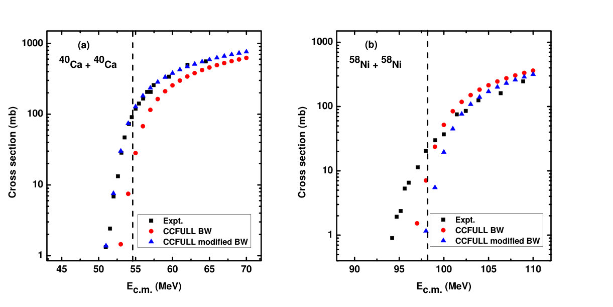 Figure 1
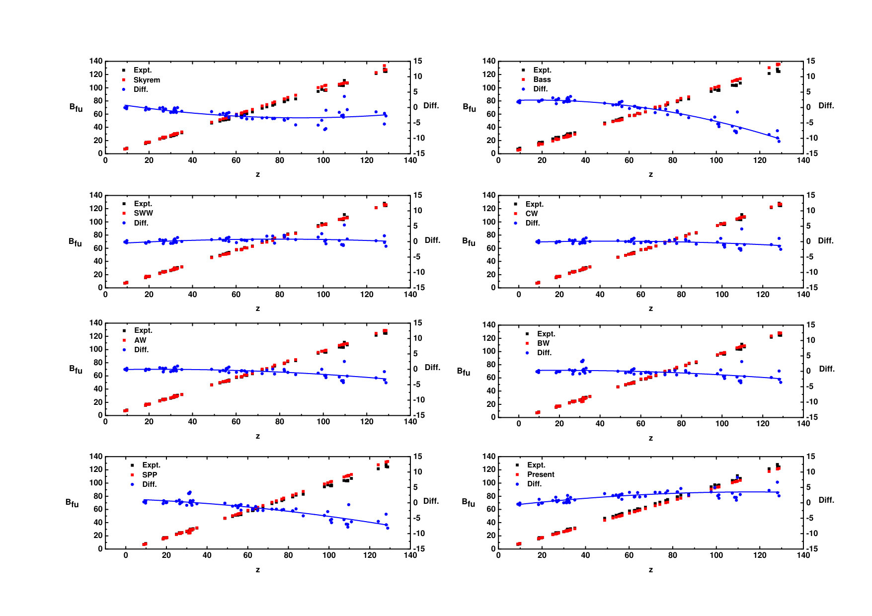 Figure 2
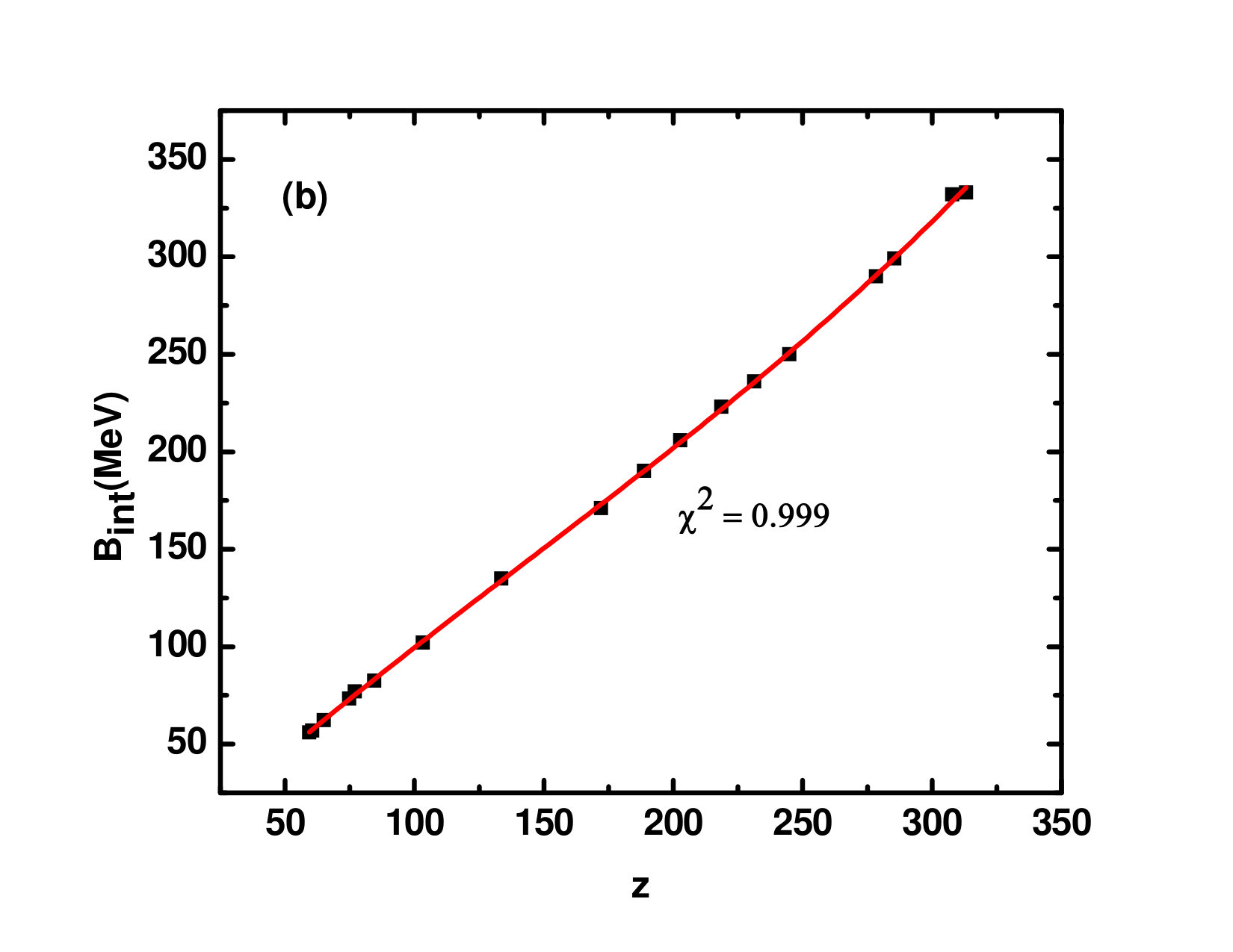 Figure 3
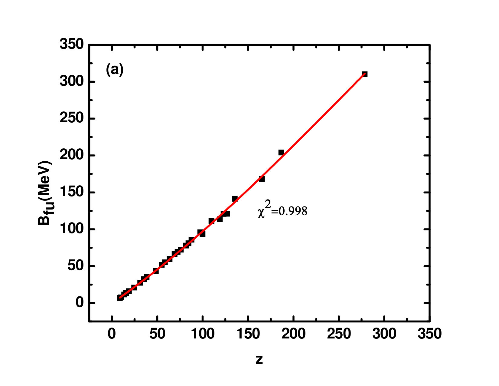 Figure 4
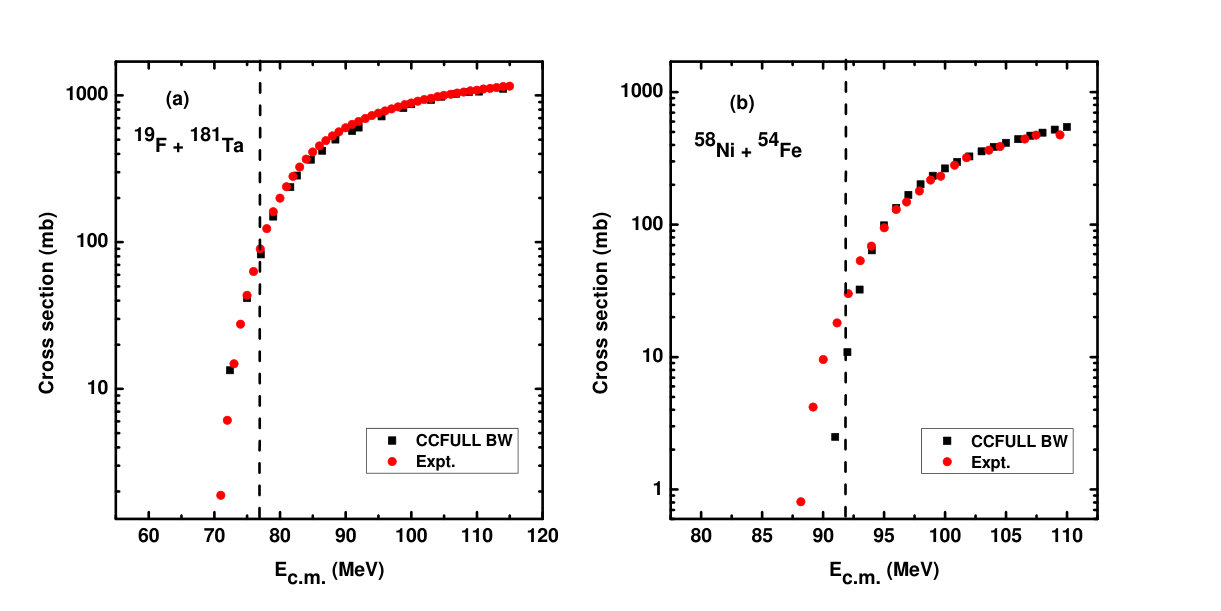 Figure 5
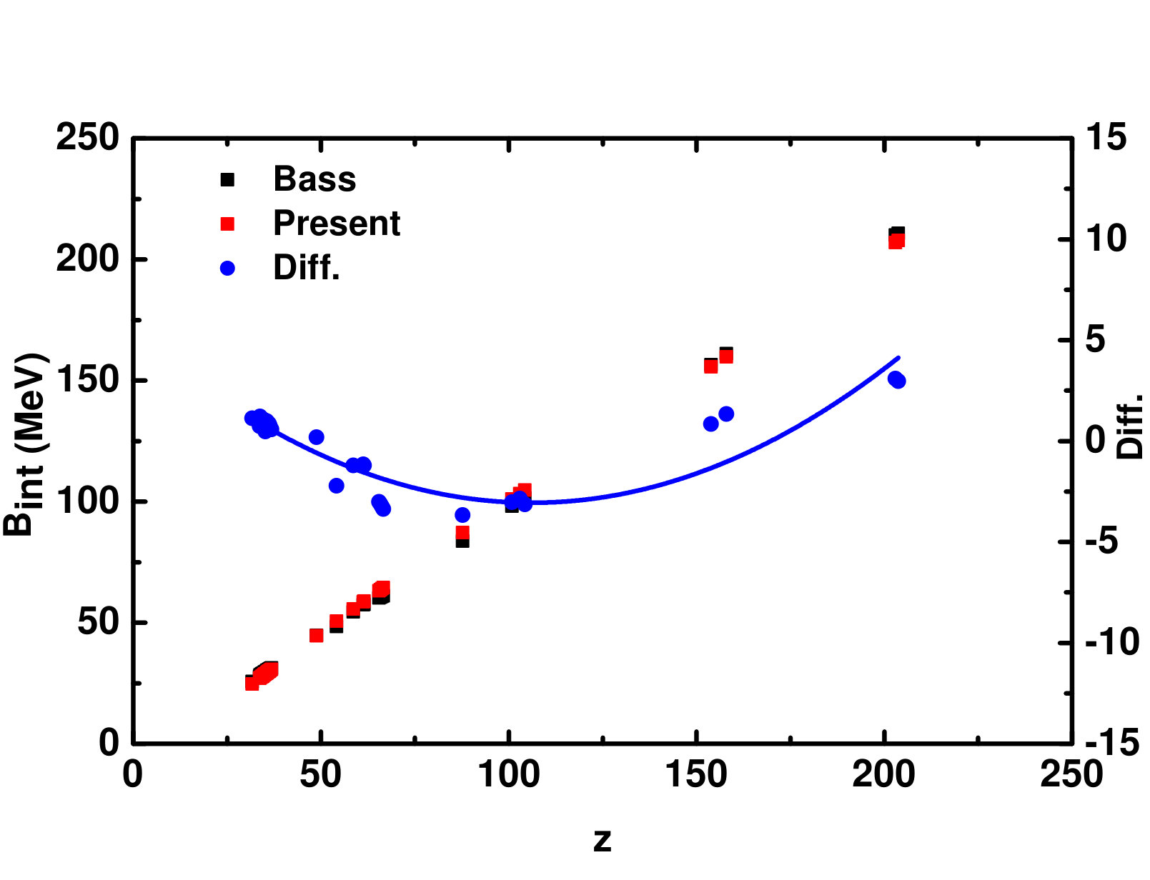 Figure 6
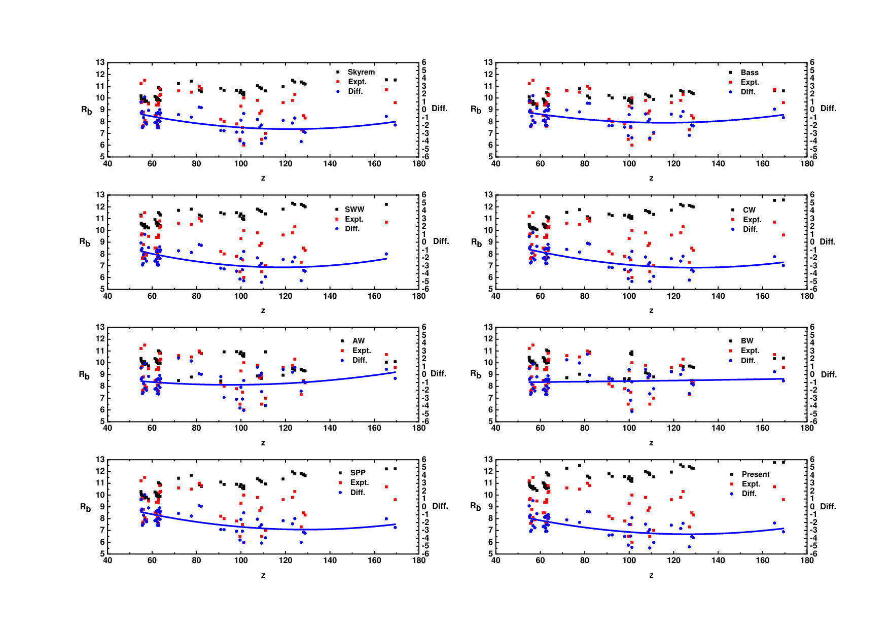 Figure 7
| System | ||
|---|---|---|
| 12C+15N | 8.83 | 6.80 [28] |
| 12C+16O | 9.98 | 7.50 [30] |
| 12C+26Mg | 13.71 | 11.5 [59] |
| 12C+30Si | 15.57 | 13.2 [60] |
| 16O+27Al | 18.84 | 43.6 [31] |
| 24Mg+26Mg | 24.63 | 20.8 [62] |
| 26Mg+32S | 31.28 | 27.5 [63] |
| 12C+92Zr | 35.27 | 32.3 [48] |
| 16O+72Ge | 38.32 | 35.4 [64] |
| 32S+40Ca | 48.52 | 43.3 [46] |
| 48Ca+48Ca | 55.03 | 51.7 [46] |
| 27Al+70Ge | 58.42 | 55.1 [46] |
| 32S+58Ni | 63.58 | 59.5 [32] |
| 40Ar+58Ni | 69.13 | 66.32[46] |
| 37Cl+73Ge | 72.42 | 69.20[46] |
| 40Ca+62Ni | 75.90 | 72.3 [60] |
| 32S+89Y | 81.68 | 77.8 [53] |
| 16O+238U | 84.43 | 80.8 [46] |
| 28Si+120Sn | 87.84 | 85.9 [46] |
| 48Ca+96Zr | 97.41 | 95.9[56] |
| 40Ca+96Zr | 100.01 | 93.6 [32] |
| 40Ar+121Sb | 109.72 | 111 [38] |
| 40Ca+124Sn | 118.95 | 113 [39] |
| 28Si+198Pt | 123.18 | 121 [40] |
| 40Ar+154Sm | 127.11 | 121 [36] |
| 40Ar+165Ho | 135.43 | 141.4[46] |
| 40Ca+192Os | 165.42 | 168.1[46] |
| 84Kr+116Cd | 186.67 | 204 [41] |
| 74Ge+232Th | 278.45 | 310 [41] |
| System | ||
|---|---|---|
| 12C+205Ti | 59.37 | 56.0[42] |
| 12C+209Bi | 60.55 | 57.0[42] |
| 12C+238U | 65.04 | 62.2[43] |
| 14N+238U | 74.82 | 73.4[43] |
| 16O+205Ti | 76.99 | 77.0[42] |
| 16O+238U | 84.43 | 82.5[43] |
| 20Ne+238U | 103.23 | 102[43] |
| 40Ar+164Dy | 133.57 | 135[44] |
| 40Ar+238U | 172.19 | 171[3] |
| 48Ti+208Pb | 188.72 | 190.1[14] |
| 54Cr+208Pb | 202.78 | 205.8[14] |
| 56Fe+208Pb | 218.65 | 223[14] |
| 58Ni+208Pb | 231.33 | 236[14] |
| 70Zn+208Pb | 244.86 | 250.6[14] |
| 84Kr+232Th | 307.86 | 332[3] |
| 84Kr+238U | 313.14 | 333[45] |
| System | ||||||||||
|---|---|---|---|---|---|---|---|---|---|---|
| 12C+14N | 8.93 | 7.00 [28] | ||||||||
| 12C+18O | 9.77 | 7.45 [29] | ||||||||
| 12C+17O | [46] | |||||||||
| 20Ne+20Ne | [61] | |||||||||
| 4He+164Dy | [46] | |||||||||
| 18O+28Si | [46] | |||||||||
| 16O+28Si | [46] | |||||||||
| 24Mg+24Mg | [59] | |||||||||
| 6Li+144Sm | [46] | |||||||||
| 7Li+159Tb | [46] | |||||||||
| 16O+40Ca | [59] | |||||||||
| 26Mg+30Si | [46] | |||||||||
| 14N+59Co | [47] | |||||||||
| 26Mg+34S | [63] | |||||||||
| 24Mg+34S | [63] | |||||||||
| 30Si+30Si | [64] | |||||||||
| 24Mg+32S | [63] | |||||||||
| 6Li+208Pb | [46] | |||||||||
| 28Si+30Si | [62] | |||||||||
| 28Si+28Si | [62] | |||||||||
| 20Ne+40Ca | [46] | |||||||||
| 24Mg+35Cl | [46] | |||||||||
| 16O+58Ni | [46] | |||||||||
| 12C+152Sm | [46] | |||||||||
| 18O+124Sn | [46] | |||||||||
| 16O+116Sn | [46] | |||||||||
| 30Si+64Ni | [65] | |||||||||
| 30Si+62Ni | [65] | |||||||||
| 28Si+64Ni | [65] | |||||||||
| 28Si+62Ni | [65] | |||||||||
| 40Ca+48Ca | [46] | |||||||||
| 28Si+58Ni | [65] | |||||||||
| 12C+204Pb | [46] | |||||||||
| 40Ca+48Ti | [50] | |||||||||
| 35Cl+54Fe | [46] | |||||||||
| 16O+144Sm | [51] | |||||||||
| 37Cl+64Ni | [46] | |||||||||
| 46Ti+46Ti | [46] | |||||||||
| 16O+186W | [51] | |||||||||
| 28Si+92Zr | [48] | |||||||||
| 40Ca+58Ni | [60] | |||||||||
| 16O+208Pb | [55] | |||||||||
| 48Ti+58Ni | [52] | |||||||||
| 36S+90Zr | [54] | |||||||||
| 19F+197Au | [46] | |||||||||
| 35Cl+92Zr | [48] | |||||||||
| 35Cl+106Pd | [46] | |||||||||
| 32S+116Sn | [46] | |||||||||
| 58Ni+60Ni | [46] | |||||||||
| 40Ca+90Zr | [46] | |||||||||
| 58Ni+58Ni | 101.27 | 95.8 [33] | ||||||||
| 40Ar+122Sn | 107.40 | 103.6 [35] | ||||||||
| 40Ar+116Sn | 108.47 | 103.3 [36] | ||||||||
| 40Ar+112Sn | 109.22 | 104.0 [36] | ||||||||
| 64Ni+74Ge | 109.29 | 103.2 [36] | ||||||||
| 40Ar+121Sb | 109.72 | 111.0 [37] | ||||||||
| 58Ni+74Ge | 111.04 | 106.8 [37] | ||||||||
| 34S+168Er | 124.24 | 121.5 [21] | ||||||||
| 28Si+208Pb | [57] | |||||||||
| 40Ar+148Sm | 128.14 | 124.7 [36] | ||||||||
| 40Ar+144Sm | 128.85 | 124.4 [36] |
| System | ||||||||||
|---|---|---|---|---|---|---|---|---|---|---|
| 48Ca+48Ca | 55.03 | 11.20 | ||||||||
| 30Si+64Ni | 55.16 | 9.60 | ||||||||
| 30Si+62Ni | ||||||||||
| 28Si+64Ni | ||||||||||
| 28Si+62Ni | ||||||||||
| 30Si+58Ni | ||||||||||
| 40Ca+48Ca | ||||||||||
| 28Si+58Ni | ||||||||||
| 40Ca+44Ca | ||||||||||
| 40Ca+40Ca | ||||||||||
| 36S+64Ni | ||||||||||
| 34S+64Ni | ||||||||||
| 40Ca+50Ti | ||||||||||
| 40Ca+48Ti | ||||||||||
| 32S+64Ni | ||||||||||
| 36Si+58Ni | ||||||||||
| 40Ca+46Ti | ||||||||||
| 16O+154Sm | ||||||||||
| 34S+58Ni | ||||||||||
| 17O+144Sm | ||||||||||
| 16O+148Sm | ||||||||||
| 32S+58Ni | ||||||||||
| 16O+144Sm | ||||||||||
| 16O+186W | ||||||||||
| 16O+208Pb | ||||||||||
| 36S+96Zr | ||||||||||
| 36S+90Zr | ||||||||||
| 36S+110Pd | ||||||||||
| 32S+110Pd | ||||||||||
| 64Ni+64Ni | ||||||||||
| 58Ni+64Ni | 9.79 | |||||||||
| 40Ca+96Zr | ||||||||||
| 58Ni+60Ni | ||||||||||
| 40Ca+90Zr | ||||||||||
| 58Ni+58Ni | ||||||||||
| 40Ar+122Sn | ||||||||||
| 40Ar+116Sn | ||||||||||
| 40Ar+112Sn | ||||||||||
| 64Ni+74Ge | ||||||||||
| 58Ni+74Ge | ||||||||||
| 40Ca+124Sn | ||||||||||
| 28Si+198Pt | ||||||||||
| 34S+168Er | ||||||||||
| 40Ar+154Sm | ||||||||||
| 40Ar+148Sm | ||||||||||
| 40Ar+144Sm | ||||||||||
| 40Ca+192Os | ||||||||||
| 40Ca+194Pt |
| Systems | B.W. Model | Others | Ref. | ||||
|---|---|---|---|---|---|---|---|
| 19F+181Ta | 60.34 | 0.63 | 1.20 | 104.5 | 0.70 | 1.12 | [67] |
| 48Ca+96Zr | 67.67 | 0.63 | 1.209 | 104.5 | 0.68 | 1.198 | [68] |
| 16O+154Sm | 57.45 | 0.63 | 1.197 | 100.0 | 1.06 | 1.019 | [69] |
| 19F+208Pb | 61.12 | 0.63 | 1.204 | 100.0 | 1.062 | 1.059 | [69] |
| 16O+208Pb | 59.20 | 0.63 | 1.201 (1.23) | 104.5 | 0.68 | 1.20 | [68] |
| 48Ca+48Ca | 60.15 | 0.63 | 1.198 | 104.5 | 0.68 | 1.185 | [68] |
| 58Ni+54Fe | 66.90 | 0.63 | 1.203 | 104.5 | 0.68 | 1.198 | [68] |
| 64Ni+64Ni | 68.49 | 0.63 | 1.208 | 104.5 | 0.68 | 1.205 | [68] |
| 24Mg+30Si | 50.52 | 0.63 | 1.172 (1.20) | 104.5 | 0.68 | 1.190 | [68] |
| 36S+90Zr | 64.85 | 0.63 | 1.204 (1.24) | 100.0 | 0.97 | 1.07 | [69] |
| 58Ni+58Ni | 67.81 | 0.63 | 1.205 (1.19) | 104.5 | 0.68 | 1.180 | [68] |
| 40Ca+40Ca | 59.09 | 0.63 | 1.191 (1.24) | 104.5 | 0.68 | 1.191 | [68] |
| System | |||
|---|---|---|---|
| 32S+24Mg | |||
| 32S+27Al | |||
| 18O+64Ni | |||
| 18O+62Ni | |||
| 18O+60Ni | |||
| 16O+64Ni | |||
| 18O+58Ni | |||
| 16O+62Ni | |||
| 16O+60Ni | |||
| 18O+65Cu | |||
| 18O+58Ni | |||
| 18O+63Cu | |||
| 35Cl+27Al | |||
| 16O+65Cu | |||
| 18O+70Zn | |||
| 16O+63Cu | |||
| 18O+68Zn | |||
| 18O+66Zn | |||
| 16O+70Zn | |||
| 18O+64Zn | |||
| 16O+68Zn | |||
| 16O+66Zn | |||
| 16O+64Zn | |||
| 12C+152Sm | |||
| 35Cl+48Ti | |||
| 16O+134Ba | |||
| 16O+150Nd | |||
| 16O+148Nd | |||
| 35Cl+64Ni | |||
| 35Cl+62Ni | |||
| 35Cl+60Ni | |||
| 35Cl+58Ni | |||
| 35Cl+90Zr | |||
| 40Ar+110Pd | |||
| 35Cl+124Sn | |||
| 35Cl+116Sn | |||
| 40Ar+197Au | |||
| 40Ar+208Pb | |||
| 54Cr+207Pb | |||
| 52Cr+208Pb |
Peer Reviews
No public reviews on file for this paper yet. If you reviewed it on a platform where reviews are public (OpenReview, ICLR, NeurIPS, ICML), you can paste yours below so the community can read it here.
Videos
No videos yet. Explain this paper in a talk, walkthrough, or lecture? Add one.
Taxonomy
TopicsNuclear physics research studies · Nuclear Physics and Applications · High-pressure geophysics and materials
Exploring the accurate nuclear potential
D.K. Swami, Yash Kumar
T. Nandi
Inter University Accelerator Centre, New Delhi-110067
Abstract
We have constructed empirical formulae for fusion and interaction barrier heights using experimental values available in the literature. Fusion excitation function measurements are used for the former and back angle quasi-elastic excitation function for the latter case. The fusion barriers so obtained have been compared with various model predictions such as Bass potential, Christenson and Winther, Broglia and Winther, Aage Winther, Siwek-Wilczyńska and J.Wilczyński, Skyrme energy density function model, and the Sao Paulo optical potential along with experimental results. The comparison allows us to find the best model, which is found to be the Broglia and Winther model. Further, to examine its predictability, the Broglia and Winther model parameters are used to obtain total fusion cross sections showing good agreement with the experimental values for beam energies above the fusion barriers. Thus, this model can be useful for planning any experiments, especially ones aiming for super heavy elements. Similarly, current interaction barrier heights have also been compared with the Bass potential model predictions. It shows that the present model calculations are much lower than the Bass potential model predictions. We believe the current interaction barrier model prediction will be a good starting point for future quasi-elastic scattering experiments. Whereas both the Broglia and Winther model and our interaction barrier model will have practical implications in carrying out physics research near the Coulomb barrier energies.
PACS numbers
24.10.-i, 25.70.Jj, 25.70.Bc, 21.30.Fe, 25.55.Ce
I Introduction
The basic characteristics of nuclear reactions are usually described by an interaction consisting of a repulsive Coulomb potential term and a short ranged attractive nuclear potential term. The resultant potential can be expressed as a function of the distance between the centres-of-mass of the target and projectile nuclei. When a projectile approaches the target nucleus it experiences a maximum force at a certain distance where the repulsive and attractive forces cannot balance each other, the repulsive Coulomb force is always higher. The projectile needs to overcome the barrier for coming close to the target nucleus. This barrier is referred to the fusion barrier , which is a basic parameter in describing the nuclear fusion reactions. The kinetic energy of the projectile must be adequate to surmount this barrier in order to enter a pocket at the adjacent to the barrier at a shorter distance, where the nuclei undergo nuclear fusion processes. The barrier is determined by the excitation function measurement of nuclear fusion [1], whereas it is estimated by many theoretical models such as Bass potential model [2; 3], proximity potential model [4], double folding model [5], Woods-Saxon potential model [6], and semi-empirical models such as Christenson and Winther (CW) model [7], Broglia and Winther (BW) model [8], Aage Winther (AW) model [9], Denisov potential (DP) model [10], Siwek-Wilczyńska and Wilczyński (SWW) model [11], Skyrme potential model [12], and the Sao Paulo optical potential (SPP)[13].
The quasi-elastic (QEL) processes involving relatively small energy transfer to excite only nuclear levels in either one of the participating nuclei or in both become significant as soon as the two bodies approach within the range of the nuclear forces. The position where the resultant of the Coulomb and nuclear forces is still repulsive and additional energy is required to get the two bodies interacting over their mutual potential barrier. This barrier is hitherto somewhat smaller than the fusion barrier and is known as the interaction barrier , which is measured by the excitation function studies of QEL scattering experiment [14]. Obviously, the two barriers are different from each other as one is characterized by the fusion reaction and the other by the QEL scatterings [2; 3]. However, many-a-time the distinction is overlooked, for example, [14; 15]. Worth noting here that it is only the Bass model [2; 3] which can estimate the interaction barriers in addition to the fusion barriers.
Recently Sharma and Nandi [16] demonstrated the coexistence of the atomic and nuclear phenomenon on the elastically scattered projectile ions while approaching the Coulomb barrier. Here the projectile ion x-ray energies were measured as a function of ion beam energies for three systems 12C(56Fe,56Fe), 12C(58Ni,58Ni) and 12C(63Cu,63Cu) and observed unusual resonance like structures as the beam energy approaching the fusion barrier energy according to the Bass model [2; 3]. We expected the resonance near to interaction barrier as this technique resembled the quasi-elastic (QEL) scattering experiment [14]. To resolve this anomaly, we planned to examine both the fusion and interaction barriers in greater detail.
At present many experiments exist in the literature for the measurements of the fusion and interaction barrier heights. In this work, we have constructed an empirical formula for estimating the fusion barriers from the fusion excitation function measurements alone and another for the interaction barriers from the QEL scattering experiments only. In the next step, we have compared the empirical results so obtained with the predictions from the various models based on proximity type of potentials such as Bass potential [2; 3] and Christenson and Winther (CW) [7] and Woods-Saxon type of potentials such as Broglia and Winther (BW) [8], Aage Winther (AW) [9], Siwek-Wilczyńska and Wilczyński (SWW) [11], Skyrme Potential (SP) [12] models, and the Sao Paulo optical potential (SPP) [13]. This comparison suggests for the need for further measurements in certain specified regions for both the cases. It is seen that this work will be useful in various applications [1], for example, correct prediction of may play important roles in experiments for the formation of super heavy elements [17] and that of finds its significance in physics research near the Coulomb barriers [16].
II Determination of the barrier heights
The fusion cross section is plotted as a function of the beam energy to obtain the excitation function curve for the corresponding reaction. Whereas the fusion barrier is obtained from the barrier distribution plot, which is defined as the second derivative of the energy-weighted cross section versus beam energy in the center-of-mass frame [18]. Many articles report only the excitation function, in such cases the fusion cross section and corresponding beam energy have been multiplied to plot against the beam energy to obtain the double derivative. The plot against beam energy have been fitted with the Gaussian function to obtain the fusion barrier heights.
Similarly, the interaction barrier can be obtained from the QEL excitation function studies as follows. The QEL scattering is affected by the sum of elastic, inelastic, and transfer processes, which is measured at backward angles of nearly , where the head-on collisions are dominant. The barrier distribution is obtained by taking the first derivative, with respect to the beam energy, of the QEL cross-section relative to the Rutherford cross section, that is, [19]. This method has been examined in several intermediate-mass systems [20; 21]. One can notice that the QEL barrier distribution behaves similarly to the fusion barrier distribution, although the former is less sensitive to the nuclear structure effects.
III General background
Theoretically, the total nucleus-nucleus interaction potential between the projectile and target nuclei, in general, is given by
[TABLE]
Where the first term is the model dependent nuclear potential, the second is centrifugal potential, where is the reduced mass of the projectile mass and the target nuclei mass in MeV/ units and represents the angular momentum of the two body system. When we consider the fusion barrier of the system, is set to zero which means the centrifugal or the second term is zero. The third term is the Coulomb potential similar to [22] and given by
[TABLE]
Where the fusion barrier radius = ( + ), depends on the system as discussed below and and are mass of projectile and target nuclei, respectively. Putting the first term of equation (1) from any particular model, one can get the fusion barrier radius, by using the condition
[TABLE]
and
[TABLE]
Hence, = and similarly, = , where is the interaction barrier radius. Of course, in equation (1) can be replaced by appropriate one, for the interaction barrier case as done in Bass potential model [2].
IV Nuclear potential models
We shall briefly discuss different models for including one developed from fully experimental results in the present work.
IV.1 Present empirical model
According to the definition for the Coulomb potential given above, the shape of the nuclear potential discussed below and representation of nuclear distances, for example, one given above for the barrier radius, and may be written as a function of , , and . Hence, the experimentally obtained from fusion excitation function measurements and from QEL measurements can be plotted against , where , as shown in Fig.1(a) and Fig.1(b), respectively. The fusion experiments used for Fig. 1 (a) and the QEL experiments used for Fig. 1(b) are given in Table I and II, respectively. Fusion data are available for , whereas QEL data for . We can notice that both vs and vs are nonlinear. The whole range of data can either be fitted with two straight lines or a third-degree polynomial to obtain the reduced chi-square nearly equal to one. Nevertheless, the later fitting is found to be somewhat better and is thus used in this work.
The polynomial function that fits the fusion excitation function data is as follows:
[TABLE]
and the other function that fits the vs data is given below:
[TABLE]
The empirical formula given in equation (5) can predict for any system within . Such predictions have been compared with different models. Similarly, the values obtained from equation (6) we collated with the predictions of the Bass model.
To obtain , we follow the following method. The barrier height can be given as
[TABLE]
and at
[TABLE]
This equation can be written in terms of
[TABLE]
For instance, if we assume in the form of Woods-Saxon potential and it is not clearly a function of , assumed to be a constant. Hence, the derivative of the above equation w.r.t. is as follows.
[TABLE]
Now we replace from equation (5) we get
[TABLE]
and thus the barrier radius .
IV.2 Bass potential model
Bass potential model [2; 3] suggests that the Coulomb barrier for quasi-elastic surface reaction is in general different from the Coulomb barrier for fusion. The former results from the quasi-elastic processes, where no mass or energy transfer takes place, whereas both mass and energy can transfer in the latter. Further, the quasi-elastic processes become significant as the projectile and target nuclei approach to the range of nuclear forces, where the resultant of the Coulomb and nuclear forces is still repulsive. Thus additional energy is required to get the nuclei within the resultant attractive force, where the fusion can occur. According to the Bass model, the barriers responsible in the quasi-elastic reactions is called the interaction barrier and it can be determined from the elastic scattering experiments [14]. The other barrier is significant in fusion reactions and is defined as the fusion barrier . The latter is equal to the height of the potential barrier for zero angular momentum.
The total effective Bass potential consists of a Coulomb, nuclear and centrifugal terms,
[TABLE]
Where is the range of nuclear interaction. The influence of fragment (projectile or target nuclei) properties on this potential can be expressed in terms of the dimensionless parameters
[TABLE]
[TABLE]
Where is the ratio of the Coulomb force to the nuclear force and is the ratio of the centrifugal force to the nuclear force at the point of contact i.e., , =1.07 fm. Here, =17.23 MeV is the surface constant as used in the liquid drop model of fission, the mass of a nucleon, and the mass number of projectile and target nuclei, respectively and other notations have usual significance. Whereas acts at = + , is the fusion distance. The is applicable for an interaction distance between the two surfaces or the centre to centre distance, = + . The is always longer than the .
The fusion distance can be approximately obtained from the relation
[TABLE]
The varies with the fragments in the nuclear interactions. The barriers and can be obtained from
[TABLE]
[TABLE]
[TABLE]
Here, it is assumed that is independent of the mass of the nuclei. Hence, from the above relations, we get .
IV.3 Christenson and Winther model
Christenson and Winther [7] derived the nucleus-nucleus interaction potential on the basis of semi classical arguments as given by
[TABLE]
where = , and is the diffuseness parameter . This form is similar to that of the Bass model [2] with different sets of radius parameter.
[TABLE]
Here, the radius of the fusion barrier has the form
[TABLE]
and the total nucleus-nucleus potential is
[TABLE]
and thus, the fusion barrier can be obtained from ).
IV.4 Broglia and Winther model
Broglia and Winther [8] have refined the CW potential [7] in order to make it compatible with the value of the maximum nuclear force of the proximity potential [4]. This refined force is taken as the standard Woods-Saxon potential given by
[TABLE]
with and
[TABLE]
Here the nucleus radius is given by:
[TABLE]
The surface energy coefficient () has the form
[TABLE]
Where = and . The total interaction potential of the two heavy ions is
[TABLE]
and it displays a maximum, i.e., the fusion barrier and the barrier radius is the solution of the following equation
[TABLE]
and is the fusion barrier.
IV.5 Aage Winther model
Aage Winther [9] adjusted slightly the parameters of the Broglia and Winther potential through an extensive comparison with the experimental data for heavy-ion elastic scattering. The resulting values of and are as follows:
[TABLE]
and
[TABLE]
and of the BW model is written as = only.
IV.6 Siwek-Wilczyńska and Wilczyński model
Siwek-Wilczyńska and Wilczyński [11] have used a large number of reactions to determine an effective nucleus-nucleus potential for reliable prediction of the fusion barriers for the systems that are studied. In this approach the nucleus-nucleus potential is taken also as the Woods-Saxon shape is given in equation (23). Where = and , the radius parameter is constant, is the diffuseness parameter and is the depth of the potential. The is given by
[TABLE]
Where is the shell correction energy [23] and
[TABLE]
Here is the ground state value for fusion and are the Coulomb energies [24] as follow
[TABLE]
Therefore, the equation (31) can be written as
[TABLE]
For determination of the fusion barrier, one considers the nucleus-nucleus potential in the region as
[TABLE]
For the region R<R_{p}+R_{t},e^{\big{[}\frac{R-R_{pt}}{a}\big{]}}\longrightarrow 0, the nucleus-nucleus potential takes the form
[TABLE]
Equation (35) gives thus the fusion barrier. It has only two free parameters and as is known from equation (34). These parameters are obtained by fitting the barrier heights from equation (35). The experimental values can be obtained where the measured fusion excitation functions are filled with the following expression.
[TABLE]
Where and Gaussian error integral function of the argument is
[TABLE]
The fitting gives three parameters the fusion barrier , the relative distance corresponding to the position of the approximate barrier and the width of the barrier . However, the values of and depend on the Coulomb barrier parameter , for example,
= and for
and for
and for
IV.7 Skyrme Potential model
Skyrme energy density function model (SEDFM) has been introduced by Wang [25; 26]. The total binding energy of a nucleus can be represented as the integral of the energy density function [27]
[TABLE]
where energy-density function has three parts: kinetic energy, Coulomb and nuclear interactions and is generally defined as follows
[TABLE]
Where is the kinetic energy density. The interaction potential is defined as
[TABLE]
where is the total energy of the interacting nuclear system. and are the energies of the projectile and target at completely separated distance , respectively. These energies can be calculated by the following relation
[TABLE]
[TABLE]
The densities of the neutron and proton for projectile and target can be described by the spherically symmetric Fermi function
[TABLE]
where , and are the parameters of the densities of the participating nuclei in the reactions, which are obtained by using the density-variation approach and minimizing the total energy of a single nucleus given by the SEDFM [25; 26].
Using the Skyrme energy density formalism, Zanganeh et al. [12] have constructed a pocket formula for fusion barrier heights and positions in the range 8 z 168 with respect to the charge and mass numbers of the interacting nuclei as follows:
[TABLE]
[TABLE]
We have made use of the equation (44,45) for SEDFM predictions for various reactions as shown in Table 2 and Table 3. Since, the SEDFM is based on the frozen density approximation, predicted values for each of the considered fusion systems are a bit higher than the corresponding experimental data.
IV.8 Sao Paulo optical potential
This model [13] also takes a Woods-Saxon form for the nuclear potential as given in equation (23). In the approximation of , the can be written as:
[TABLE]
where is a positive dimensionless parameter. Note that the parameter , which appears in the argument of the logarithm of the above equation, can also be written as and is larger than one in most cases. The barrier potential is given by
[TABLE]
.
V Discussion
We have constructed the empirical formulae for the fusion and interaction barrier heights using the experimental results available in the literature as mentioned above. The fusion barrier heights and fusion barrier radius can be obtained from the equation (5) and (11), respectively. The values obtained from various theoretical models for different systems, which are not used to formulate the present model, are compared with the experimental results in table III and Fig. 2. Similar comparisons have also been done for in table IV and Fig. 3. To check which model gives the best agreement with the experimental results, the differences of both and values between the experiments and models have been plotted as a function of also in Fig. 2 and 3, respectively. Further, we obtained the sum of the squared residuals (), where is the residual or difference and n is the number of data points, and mean squared error () to find the minimum mean error (). This analysis suggests that the CW model is the best and BW model is the second best for . Whereas the BW model is the best and AW the second best for . Further, the Woods-Saxon potential (equation (23)) is more sensitive to the () than and parameters. Hence, the BW model can be taken as the best model. The BW model parameters for several reactions are compared with those obtained by others in Table V. Here, an important point is to note that though the current model is made out of the experimental results, still it is not found to be the best among the eight models considered here. It happens because of the fact that there are very few data exist for .
To examine whether the BW model provides good Woods-Saxon potential, we plan to make use of the parameters , (=), and from this model as required by the CCFULL calculations [66] to obtain the total fusion cross sections and compare them with the experimental results. However, the radius parameters used in the BW model does not include . To introduce it there we rewrite equation (23) as follows:
[TABLE]
Here and are taken from equation (25).
We have used such Woods-Saxon potential parameters for many reactions in the CCFULL calculations without taking the coupling between the relative motion of colliding nuclei and the intrinsic degrees of freedom into account and compared with the experimental total fusion cross sections. Most of them give very good agreements at the beam energies larger than the fusion barriers as shown for two systems 19F+181Ta and 58Ni+54Fe in Fig.5. However, sometimes certain departure has also been found for example 40Ca+40Ca and 58Ni+58Ni systems as shown in Fig.6. Note that the BW model parameters underestimate the measured cross sections for 40Ca+40Ca and overestimates for 58Ni+58Ni reaction. A small variation of the value of turns the agreement good. In the case of 40Ca+40Ca, value of has to be increased from 1.19 to 1.24 fm and for 58Ni+58Ni, the value of has to be decreased from 1.205 to 1.19 fm. A comparison of the Woods-Saxon potential parameters with other works for twelve reactions is shown in Table VI. Here, the asymmetric systems show better agreement than the symmetric systems. One out five asymmetric systems and four out of seven symmetric systems are not in agreement. One noticeable fact can be seen here that some of the reactions show good agreement with the measured total fusion cross sections even till the low energy side, for example, 19F+181Ta and 40Ca+40Ca. It means these reactions do not need any coupling effects into account to increase the cross sections anymore. Whereas, the total fusion cross sections with the potential parameters used in [67] require the coupling effects to have agreements with the measured data. On the other hand, some reactions such as 58Ni+58Ni and 58Ni+54Fe require the coupling effects as usual [68]. One point may be worth noting that sometimes the CCFULL calculation does not reproduce the measured fusion cross sections and the measurement have been altered by introducing an “efficiency factor” so as to find the agreement [69]. In contrast, we notice a little variation of the parameter gives good agreement.
Next, the interaction barrier heights can be obtained from equation (6) to compare with the experiments and models. However, the measurements are very limited and all the experimental values have been used to construct the present interaction barrier model. Hence, the current values have only been compared with the Bass potential model predictions in table VI and Fig.4. Differences of the current model values from the Bass model predictions shown in the figure suggest that the present model are quite lower than the Bass potential model predictions throughout the z values except for z 100.
VI Conclusion
In this paper, using the experimental values available in the literature, empirical formulae for fusion and interaction barrier heights as well as barrier radii are introduced. The present study is restricted to the fusion and interaction reactions in the regime and , respectively. We have carried out a comparative study of the fusion barrier as well as barrier radius between present empirical formula and various empirical and semi-empirical models along with experimental results. According to a thorough comparison with the experimental values, it is found that the Broglia and Winther model gives reasonable barrier heights in comparison with the present empirical model and various empirical and semi-empirical models. Further, to examine its predictability, the Broglia and Winther model parameters are used to obtain the total fusion cross sections and compared with the experimental values. The comparison shows good agreement at the energies above the fusion barriers, but below the barriers the predictions for some reactions show a departure from the experimental results.
Similarly, current interaction barrier heights are compared with only model available the Bass potential model predictions, because of the scarcity of measurements and other model predictions. Experiments are very essential in the lower z range. Whatsoever, the comparison shows that the present model predictions are much lower than the Bass potential model values. We believe the current model can be used as a guideline for estimating the interaction barrier heights for the future measurements even beyond the working range of the model by extrapolation.
Acknowledgements: We would like to acknowledge the illuminating discussions with Subir Nath, Ambar Chatterjee, B.R. Behra and S. Kailas.
The reference list from the paper itself. Each links out to its DOI / PubMed record.
- 1[1] B. B. Back, H. Esbensen, C. L. Jiang and K. E. Rehm, Rev. Mod. Phys. 86, 317 (2014).
- 2[2] R. Bass, Nucl. Phys. A 231, 45 (1974).
- 3[3] R Bass, Phys. Lett. 47, 139 (1973).
- 4[4] J. Blocki, J. Randrup, W. J. Swiatecki, and C. F. Tsang, Annals of Physics 105, 427 (1977).
- 5[5] G.R. Satchler, W.G. Love, Physics Reports 55, 183 (1979).
- 6[6] D. S. Saxon and R. D. Woods, Physical Review , 577 (1954).
- 7[7] P. R. Christensen and A. Winther, Phys. Lett. 65B, 19 (1976).
- 8[8] W. Reisdorf, J.Phys. G:Nucl.Part.Phys. 20, 1297 (1994).