On the design of new classes of fixed-time stable systems with predefined upper bound for the settling time
R. Aldana-L\'opez, D. G\'omez-Guti\'errez, E. Jim\'enez-Rodr\'iguez,, J. D. S\'anchez-Torres, M. Defoort

TL;DR
This paper introduces a methodology for designing fixed-time stable systems with a predefined upper bound on settling time, improving over traditional methods by reducing conservativeness and providing a broad class of such systems.
Contribution
It presents a novel construction procedure for fixed-time stable systems with predefined and minimal upper bounds on settling time using time-scale transformations and Lyapunov analysis.
Findings
Generated new fixed-time stable algorithms with predefined upper bounds.
Provided conditions for the least possible upper bound of settling time.
Demonstrated effectiveness through illustrative examples.
Abstract
This paper aims to provide a methodology for generating autonomous and non-autonomous systems with a fixed-time stable equilibrium point where an Upper Bound of the Settling Time (UBST) is set a priori as a parameter of the system. In addition, some conditions for such an upper bound to be the least one are provided. This construction procedure is a relevant contribution when compared with traditional methodologies for generating fixed-time algorithms satisfying time constraints since current estimates of an UBST may be too conservative. The proposed methodology is based on time-scale transformations and Lyapunov analysis. It allows the presentation of a broad class of fixed-time stable systems with predefined UBST, placing them under a common framework with existing methods using time-varying gains. To illustrate the effectiveness of our approach, we generate novel, autonomous and…
Click any figure to enlarge with its caption.
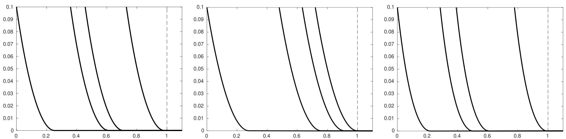 Figure 1
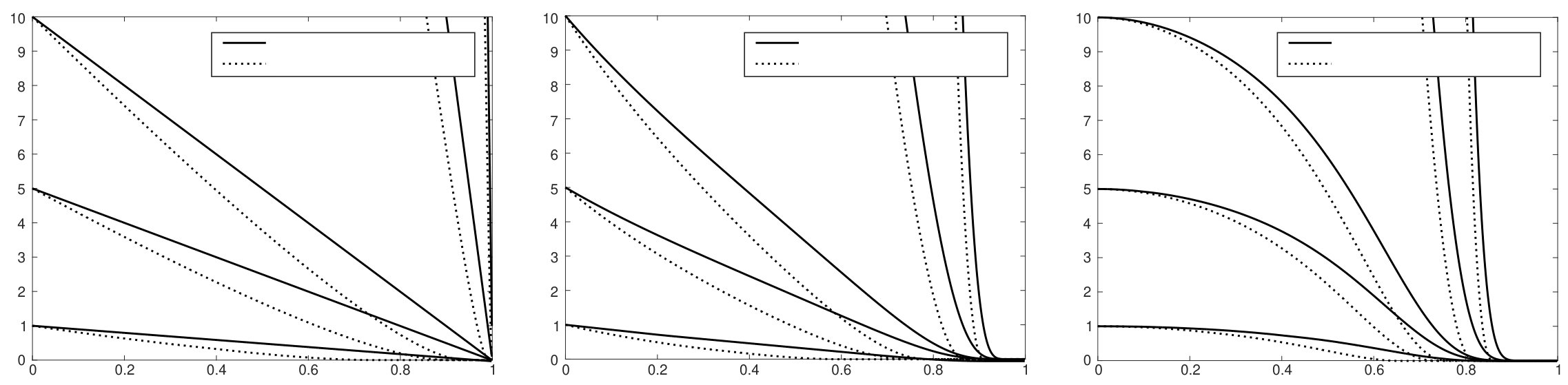 Figure 2
| Conditions | |||
|---|---|---|---|
| (i) | , , , | ||
| (ii) | |||
| (iii) | |||
| (iv) | , and |
| Conditions | ||
|---|---|---|
| (i) | and is and | |
| (ii) | is and | |
| (iii) | is and | |
| (iv) | , , , , , , is , |
Peer Reviews
No public reviews on file for this paper yet. If you reviewed it on a platform where reviews are public (OpenReview, ICLR, NeurIPS, ICML), you can paste yours below so the community can read it here.
Videos
No videos yet. Explain this paper in a talk, walkthrough, or lecture? Add one.
Generating new classes of fixed-time stable systems with predefined upper bound for the settling time111This is the preprint version of the accepted manuscript: Rodrigo Aldana-López, David Gómez-Gutiérrez, Esteban Jiménez-Rodríguez, Juan Diego Sánchez-Torres and Michael Defoort “Generating new classes of fixed-time stable systems with predefined upper bound for the settling time”. International Journal of Control. 2021. DOI: 10.1080/00207179.2021.1936190.
Please cite the publisher’s version. For the publisher’s version and full citation details see: https://doi.org/10.1080/00207179.2021.1936190. The following links provide access, for a limited time, to a free copy of the publisher’s version: Link 1. Link 2. Link 3. Link 4.
\nameRodrigo Aldana-Lópeza, David Gómez-Gutiérrezb,c, Esteban Jiménez-Rodríguezd, Juan Diego Sánchez-Torrese and Michael Defoortf CONTACT D. Gómez-Gutiérrez. Email: [email protected] aDepartment of Computer Science and Systems Engineering, University of Zaragoza, Zaragoza, Spain; b Multi-Agent Autonomous Systems Lab, Intel Labs, Intel Tecnología de México, Jalisco, Mexico; c Tecnologico de Monterrey, Escuela de Ingeniería y Ciencias, Jalisco, Mexico; d Relativity6 Inc. Computer Science & Artificial Intelligence Lab., Jalisco, Mexico; e Research Laboratory on Optimal Design, Devices and Advanced Materials -OPTIMA-, Department of Mathematics and Physics, ITESO, Jalisco, Mexico; f LAMIH, UMR CNRS 8201, INSA, Polytechnic University of Hauts-de-France, Valenciennes, France.
Abstract
This paper aims to provide a methodology for generating autonomous and non-autonomous systems with a fixed-time stable equilibrium point where an Upper Bound of the Settling Time (UBST) is set a priori as a parameter of the system. In addition, some conditions for such an upper bound to be the least one are provided. This construction procedure is a relevant contribution when compared with traditional methodologies for generating fixed-time algorithms satisfying time constraints since current estimates of an UBST may be too conservative. The proposed methodology is based on time-scale transformations and Lyapunov analysis. It allows the presentation of a broad class of fixed-time stable systems with predefined UBST, placing them under a common framework with existing methods using time-varying gains. To illustrate the effectiveness of our approach, we generate novel, autonomous and non-autonomous, fixed-time stable algorithms with predefined least UBST.
keywords:
Predefined-time systems, fixed-time systems, prescribed-time systems
††articletype: REGULAR PAPER
1 Introduction
In recent years, dynamical systems exhibiting convergence to their origin in some finite time, independent of the initial condition of the system, have attracted a great deal of attention. For this class of dynamical systems, their origin is said to be fixed-time stable, which is a stronger notion of finite-time stability (Bhat \BBA Bernstein, \APACyear2000; Moulay \BBA Perruquetti, \APACyear2006), because in the latter the settling time is, in general, an unbounded function of the initial condition of the system. This research effort has derived several contributions on algorithms with the fixed-time convergence property, such as synchronization of complex networks (Yang \BOthers., \APACyear2017; Khanzadeh \BBA Pourgholi, \APACyear2017; X. Liu \BBA Chen, \APACyear2016; Tian, Lu, Zuo\BCBL \BBA Yang, \APACyear2018; X. Liu \BOthers., \APACyear2018), stabilizing controllers (Polyakov, \APACyear2012; Polyakov \BOthers., \APACyear2015; Basin \BOthers., \APACyear2016; Zimenko \BOthers., \APACyear2018; Sánchez-Torres \BOthers., \APACyear2020; Zuo, \APACyear2019; Gómez-Gutiérrez, \APACyear2020), distributed resource allocation (Lin \BOthers., \APACyear2019), optimization (Ning, Han\BCBL \BBA Zuo, \APACyear2017), multi-agent coordination (Aldana-López, Gómez-Gutiérrez, Defoort\BCBL \BOthers., \APACyear2019; Defoort \BOthers., \APACyear2016; Zuo \BBA Tie, \APACyear2014; Wang \BOthers., \APACyear2018; Shi \BOthers., \APACyear2018; X. Liu \BOthers., \APACyear2019), state observers (Ménard \BOthers., \APACyear2017), and online differentiation algorithms (Cruz-Zavala \BOthers., \APACyear2011; Angulo \BOthers., \APACyear2013).
The fixed-time stability property is of great interest in the development of algorithms for scenarios where real-time constraints need to be satisfied. In fault detection, isolation, and recovery schemes (Tabatabaeipour \BBA Blanke, \APACyear2014), failing to recover from the fault on time may lead to an unrecoverable mode. In hybrid dynamical systems, it is frequently required that the observer (resp. controller) stabilizes the observation error (resp. tracking error) before the next switching occurs (Defoort \BOthers., \APACyear2011; Gómez-Gutiérrez \BOthers., \APACyear2015). In the frequency control of an interconnected power network, not only is the frequency deviation of interest but also how long the frequency stays out of the bounds (Mishra \BOthers., \APACyear2018).
A Lyapunov differential inequality for an autonomous system to exhibit fixed-time stability was presented in (Polyakov, \APACyear2012; Zuo \BBA Tie, \APACyear2016), together with an Upper Bound of the Settling Time (UBST) of the system trajectory. However, such an upper estimate is too conservative (Aldana-López, Gómez-Gutiérrez, Jiménez-Rodríguez\BCBL \BOthers., \APACyear2019). Only recently, non-conservative UBST has been derived (Parsegov \BOthers., \APACyear2012; Aldana-López, Gómez-Gutiérrez, Jiménez-Rodríguez\BCBL \BOthers., \APACyear2019) for some scenarios. An alternative characterization, based on homogeneity theory, was proposed in (Andrieu \BOthers., \APACyear2008; Polyakov \BOthers., \APACyear2016; Tian, Lu, Zuo\BCBL \BBA Wang, \APACyear2018). Although it is a powerful tool for the design of high order fixed-time stable algorithms, it poses a challenging design problem for time constrained scenarios, since an UBST is often unknown. Thus, the design of fixed-time stable systems where an UBST is set a priori explicitly as a parameter of the system, as well as the reduction/elimination of the conservativeness of an UBST, is of great interest. This problem has been partially addressed for autonomous systems see, e.g., (Aldana-López, Gómez-Gutiérrez, Jiménez-Rodríguez\BCBL \BOthers., \APACyear2019; Sánchez-Torres \BOthers., \APACyear2018; Aldana-López, Gómez-Gutiérrez, Defoort\BCBL \BOthers., \APACyear2019), mainly focusing on the class of systems proposed in (Polyakov, \APACyear2012; Sánchez-Torres \BOthers., \APACyear2018; Jiménez-Rodríguez \BOthers., \APACyear2018); and for non-autonomous systems, mainly focusing on time-varying gains that either become singular (Morasso \BOthers., \APACyear1997; Song \BOthers., \APACyear2018; Becerra \BOthers., \APACyear2018; Wang \BOthers., \APACyear2018; Yucelen \BOthers., \APACyear2018; Kan \BOthers., \APACyear2017) or induce Zeno behavior (Y. Liu \BOthers., \APACyear2018; Ning \BBA Han, \APACyear2018) as the predefined-time is reached.
Contributions: We provide a methodology for generating new classes of autonomous and non-autonomous fixed-time stable systems, where an UBST is set a priori explicitly as a parameter of the system. The main result is a sufficient condition in the form of a Lyapunov differential inequality, for a nonlinear system to exhibit this property. Additionally, we show that for any fixed-time stable system with continuous settling time function there exists a Lyapunov function satisfying such differential inequality. Based on this characterization, we show how a fixed-time stable system with predefined UBST can be constructed from a nonlinear asymptotically stable one, presenting sufficient conditions for such an upper bound to be the least one. To illustrate our approach, we provide examples showing how to derive autonomous and non-autonomous fixed-time stable systems, with predefined least UBST. This is a significant contribution to the design of control systems satisfying time constraints since, even in the scalar case, the existing UBST estimates are often too conservative (Aldana-López, Gómez-Gutiérrez, Jiménez-Rodríguez\BCBL \BOthers., \APACyear2019).
Notation: is the set of real numbers, , and . The Euclidean norm of is denoted as . denotes the first derivative of the function . is the class of functions with and which has continuous -th derivative in . For , is the Gamma function; for , and are the incomplete Beta function and its inverse, respectively; for is the Error function. For , and are the cosine and sine integrals respectively. is the class of strictly increasing functions with satisfying and .
2 Preliminaries
Consider the system
[TABLE]
where is the state of the system, is a parameter, and , continuous on and continuous almost everywhere on . The solutions are understood in the sense of Caratheodory (O’Regan, \APACyear1997). We assume that is such that the origin of system (1) is asymptotically stable and system (1) has the properties of existence and uniqueness of solutions in forward-time on the interval (Khalil \BBA Grizzle, \APACyear2002). The solution of (1) for with initial condition is denoted by , and the initial state is given by .
Remark 1*.*
For simplicity, throughout the paper, we assume that the origin is the unique equilibrium point of the systems under consideration. Thus, without ambiguity, we refer to the global stability (in the respective sense) of the origin of the system as the stability of the system. The extension to local stability is straightforward.
Definition 2.1**.**
(Polyakov \BBA Fridman, \APACyear2014)(Settling-time function)
The settling-time function of system (1) is defined as .
For autonomous systems ( in (1) does not depend on ), the settling-time function is independent of . Notice that, if the system is exponentially stable, then according to Definition 2.1, , .
Definition 2.2**.**
(Polyakov \BBA Fridman, \APACyear2014) (Fixed-time stability) System (1) is said to be fixed-time stable if it is asymptotically stable (Khalil \BBA Grizzle, \APACyear2002) and the settling-time function is bounded on , i.e. there exists such that if and . Thus, is an UBST of .
We are interested on finding sufficient conditions on system (1) such that an UBST is given by the parameter , i.e. . Of particular interest is to find sufficient conditions such that is the least UBST.
2.1 Time-scale transformations
As in (Picó \BOthers., \APACyear2013), the trajectories corresponding to the system solutions are interpreted, in the sense of differential geometry (Kühnel, \APACyear2015), as regular parametrized curves. Since we apply regular parameter transformations over the time variable, then without ambiguity, this reparametrization is sometimes referred to as time-scaling.
Definition 2.3**.**
(Kühnel, \APACyear2015, Definition 2.1)
A regular parametrized curve, with parameter , is a immersion , defined on a real interval . This means that holds everywhere.
Definition 2.4**.**
(Kühnel, \APACyear2015, Pg. 8)
(Regular parameter transformation) A regular curve is an equivalence class of regular parametrized curves, where the equivalence relation is given by regular (orientation preserving) parameter transformations , where is , bijective and . Therefore, if is a regular parametrized curve and is a regular parameter transformation, then and are considered to be equivalent.
3 Main Results
The methodology presented in this section to obtain fixed-time stable systems with predefined UBST subsumes some existing results, in both, the autonomous and the non-autonomous cases.
3.1 Time-scaling and settling-time computation
Assumption 3.1**.**
* is continuous in , locally Lipschitz in , and satisfies and , . Moreover, is the unique solution of the asymptotically stable system*
[TABLE]
and is its settling time.
The following lemma presents the construction of the parameter transformation that will be used hereinafter.
Lemma 3.2**.**
Under Assumption 3.1, suppose that
[TABLE]
has a unique solution on , where , and is a function such that continuous for all and . Then, the map , where is the resulting range of , is continuous and bijective. Moreover, the bijective function defined by is a parameter transformation. Furthermore, .
Proof.
Let be the solution of (3) in . Since , , is continuous, then is continuous on and is . Moreover, for all and , , then it satisfies , hence is injective (Spivak, \APACyear1965, Pg. 34). On the other hand, and , hence, by the continuity of , is surjective and . Thus, is bijective. It follows that is , satisfies and is bijective. Thus, is a parameter transformation. ∎
The following lemma shows that if (2) has a known settling time function, then the parameter transformation given in Lemma 3.2 induces a nonlinear system with known settling-time function.
Lemma 3.3**.**
Under Assumption 3.1, suppose that is the unique solution of (3) on , and let \Psi(z,\hat{t})=\left\{\begin{array}[]{ll}\Upsilon(z,\hat{t})&\text{for }\hat{t}\in\mathcal{J}=[0,\lim_{\tau\to\mathcal{T}(x_{0},0)}\psi(\tau))\\ 1&\text{otherwise}\end{array}\right. with and as in Lemma 3.2. Then, the system
[TABLE]
where , , has a unique solution
[TABLE]
where and . Moreover, (4) is asymptotically stable and the settling time of is given by
[TABLE]
Proof.
Consider the parameter transformation given in Lemma 3.2 and let . Notice that, , and , are equivalent (in the sense of regular curves). Moreover, , where and . Hence, , and therefore is solution of (4) on . Thus, for the solution , of (2), the equivalent curve , , under the parameter transformation , is solution of (4) on .
Moreover, since , then for any solution of (4) on , there exists an equivalent curve on , under the parameter transformation , that is solution of (2). Thus the uniqueness of the solution of (4) on follows from the uniqueness of solutions of (2). Finally, since reaches the origin at then, reaches the origin at . Moreover, since (4) has an equilibrium point at , then the solution of (4) remains at the origin for all . Hence, we can conclude that (4) is asymptotically stable, (5) is the unique solution in the interval and the settling time function is given by (6).
∎
3.2 Fixed-time stability of scalar systems with predefined least UBST
In the rest of the paper, we analyze the cases where is time invariant or a function only of . We show that in these cases, (3) has a unique solution.
Assumption 3.4**.**
Let be a function satisfying , , and
[TABLE]
Lemma 3.5**.**
Under Assumption 3.1, let where satisfies Assumption 3.4, then, (3) has a unique solution on , given by
[TABLE]
Proof.
Let and notice that is independent of . Therefore, it follows that
[TABLE]
has a unique solution given by . Moreover, by (Agarwal \BBA Lakshmikantham, \APACyear1993, Lemma 1.2.2), a solution of (9) is also a solution of (3) and vice versa. ∎
Assumption 3.6**.**
Let be a continuous function on satisfying (7) and , . Moreover, is either non-increasing or locally Lipschitz on .
Lemma 3.7**.**
Under Assumption 3.1, let , and consider the first order ordinary differential equation
[TABLE]
where satisfies Assumption 3.6, then (10) has a unique solution , which is bijective and given by
[TABLE]
Moreover, let then is also the unique solution of (3) on .
Proof.
It follows that (10) has a unique solution given by . Note that , is with , and , hence is injective (Spivak, \APACyear1965, Pg. 34). Note that and and, by continuity of , is surjective. Hence, is bijective. Since , then is a solution of (3). Now, on the one hand if is non-increasing, then is non-increasing. To show this let , and . On the other hand, if is Lipschitz on , then is Lipschitz on . To show this, note that there exists a constant such that where . Then, in the former (resp. in the latter) case it follows from Peano’s uniqueness Theorem (Agarwal \BBA Lakshmikantham, \APACyear1993, Theorem 1.3.1) (resp. from Lipschitz uniqueness Theorem (Agarwal \BBA Lakshmikantham, \APACyear1993, Theorem 1.2.4)) that
[TABLE]
has a unique solution , . Since , then (12) with has a unique solution , . Moreover, by (Agarwal \BBA Lakshmikantham, \APACyear1993, Lemma 1.2.2), a solution of (12) is a solution of (3) and vice versa. ∎
In Lemma 3.8, we present a characterization for a map , in the autonomous case, such that system (4) is fixed-time stable with as the least UBST.
Lemma 3.8**.**
*(Characterization of for fixed-time stability of autonomous systems with predefined least UBST)
Under Assumption 3.1, with*
[TABLE]
where and satisfies Assumption 3.4, system (4) is fixed time stable with as the predefined least UBST.
Proof.
By Lemma 3.5, (8) is the solution of (3). Using the change of variables , (6) leads to . Since then is increasing with respect to . Moreover, since satisfies (7), the settling-time function satisfies . ∎
The following result states the construction of fixed-time stable non-autonomous systems with predefined UBST.
Lemma 3.9**.**
*(Characterization of for fixed-time stability of non-autonomous systems with predefined least UBST)
Under Assumption 3.1, let , , be the solution of (10) and its inverse map. Then, with*
[TABLE]
where and satisfies Assumption 3.6, system (4) is fixed-time stable with as the predefined UBST. Furthermore,
the settling time is exactly for all if , for all ; 2. 2.
* if , but the least UBST is if, in addition, is radially unbounded, i.e. as .* 3. 3.
If (2) is fixed-time stable, then, there exists such that for all and all .
Proof.
By Lemma 3.7, the solution of (3) is given by (11). Then, the settling time function of (4) is given by . To show item (1) note that if , then , . To show item (2) note that, since then . However, if is radially unbounded, then . Hence, is the least UBST. To show item (3) notice that, since there exists , such that for all , then , such that . Thus, for all , . ∎
Remark 2*.*
Fixed-time stability of non-autonomous systems has been applied for the design of stabilizing controllers (Song \BOthers., \APACyear2018), observers (Holloway \BBA Krstic, \APACyear2019), consensus algorithms (Wang \BOthers., \APACyear2017; Colunga \BOthers., \APACyear2018; Wang \BOthers., \APACyear2018; Ning \BBA Han, \APACyear2018) and robot control (Delfin \BOthers., \APACyear2016) with predefined settling-time at , which uses time-varying gains that are either continuous in (Morasso \BOthers., \APACyear1997; Song \BOthers., \APACyear2018; Becerra \BOthers., \APACyear2018; Wang \BOthers., \APACyear2018) or piecewise continuous requiring Zeno behavior (Y. Liu \BOthers., \APACyear2018; Ning \BBA Han, \APACyear2018) as approaches . Notice that, in this paper, we focus on the former case.
Remark 3*.*
In the autonomous case, is the least UBST, whereas, in the non-autonomous case, if item (1) is satisfied, every nonzero trajectory converges exactly at . This feature has been referred in the literature as predefined-time (Becerra \BOthers., \APACyear2018), appointed-time (Y. Liu \BOthers., \APACyear2018) or prescribed-time (Wang \BOthers., \APACyear2018). However, note that , but if item (2) or (3) in Lemma 3.9 is satisfied, then the origin is reached before the singularity in occurs.
3.3 Lyapunov analysis for fixed time stability with predefined UBST
The following theorem provides a sufficient condition for a (general) nonlinear system to be fixed-time stable with predefined UBST. This result follows from the comparison lemma (Khalil \BBA Grizzle, \APACyear2002, Lemma 3.4) and the application of the above results on the time derivative of the Lyapunov candidate function.
Theorem 3.10**.**
*(Lyapunov characterization for fixed-time stability with predefined UBST)
Under Assumption 3.1, if there exists a continuous and differentiable positive definite radially unbounded function , such that its time-derivative along the trajectories of (1) satisfies*
[TABLE]
where , and is characterized by the conditions of Lemma 3.8 or Lemma 3.9, then, system (1) is fixed-time stable with as the predefined UBST. If the equality in (15) holds, then is the least UBST.
Proof.
Let be a function satisfying and , and let . Then, is the least UBST of . Moreover, by the comparison lemma (Khalil \BBA Grizzle, \APACyear2002, Lemma 3.4), it follows that . Consequently, will converge to the origin before . If (15) is an equality and , then, and is the least UBST. ∎
Theorem 3.11**.**
If system (1) is autonomous, fixed-time stable and has a continuous settling time function, then there exists a continuous positive definite function , such that its time-derivative along the trajectories of (1) satisfies (15) with characterized by the conditions of Lemma 3.8. If in addition, then is radially unbounded.
Proof.
Let , with satisfying Assumption 3.4. Note that and hence is a bijection (Spivak, \APACyear1965, Pg. 34). Moreover note that and . Hence, is a continuous and positive definite function satisfying . Furthermore, consider the trajectory , then, as noted in (Bhat \BBA Bernstein, \APACyear2000, Proposition 2.4), . Therefore, . It follows that, if then is radially unbounded. ∎
The following theorem allows generating fixed-time stable systems with predefined UBST from an asymptotically stable ones that has a Lyapunov function satisfying (17). By construction, such will also be a Lyapunov function for system (18) satisfying (15).
Theorem 3.12**.**
(Generating fixed-time stable systems with predefined UBST) Under Assumption 3.1, let the system
[TABLE]
be asymptotically stable, where , is continuous and locally Lipschitz everywhere except, perhaps, at with . If there exists a Lyapunov function for system (16) such that
[TABLE]
then, if is continuous on , where and is a function satisfying the conditions of Lemma 3.8 or Lemma 3.9, the system
[TABLE]
has a unique solution in the interval and it is fixed-time stable with as the predefined UBST.
Proof.
Since the conditions of Lemma 3.8 or Lemma 3.9 are satisfied, then, (3) has a unique solution. Hence, the proof of the existence of a unique solution for (18) follows by the same arguments as those of the proof of Lemma 3.3. Let be a Lyapunov function candidate for (16) such that (17) holds. Therefore, , . Hence, the evolution of is given by , . Hence, by Theorem 3.10, converges to the origin in fixed-time with as the predefined UBST. ∎
Notice that, the term in (4) is continuous at with any choice of from either Lemma 3.8 or Lemma 3.9, since and . However, an arbitrary selection of and may lead to a right-hand side of (18) discontinuous at the origin. A construction from a linear system, guaranteeing continuity of the right-hand side of (18) is provided in the following proposition.
Corollary 3.13**.**
Let defined as in (13) with satisfying Assumption 3.4 and , is the solution of with Hurwitz and is the largest eigenvalue of . Then, , where , is continuous, and the system
[TABLE]
where , is fixed-time stable with as the predefined UBST. Moreover, if with a positive constant and a skew-symmetric matrix then is the least UBST.
Proof.
Consider system (16) with which has a Lyapunov function satisfying . Note that, is continuous and is continuous except at the origin. Therefore, since , to check continuity, it only suffices to show that which follows from . Hence, is continuous everywhere. It follows from Theorem 3.12 that (19) is fixed-time stable with as the predefined UBST. Note that, if and , then and . Hence, by Theorem 3.10, (19) is fixed-time stable with as the least UBST. ∎
Remark 4*.*
Notice that Theorem 3.10 can be used for the design of first and second order controllers as in (Aldana-López, Gómez-Gutiérrez, Jiménez-Rodríguez\BCBL \BOthers., \APACyear2019). The design of arbitrary order controllers as in (Mishra \BOthers., \APACyear2018). The design of consensus protocols, as in (Aldana-López, Gómez-Gutiérrez, Defoort\BCBL \BOthers., \APACyear2019; Ning, Jin\BCBL \BBA Zheng, \APACyear2017); the design of non-autonomous arbitrary order controllers as in (Pal \BOthers., \APACyear2020; Gómez-Gutiérrez, \APACyear2020) or the design of non-autonomous state observers and online differention algorithms (Aldana-López \BOthers., \APACyear2020).
4 Examples of fixed-time stable systems with predefined least UBST
4.1 Examples of autonomous fixed-time stable systems with predefined least UBST
In this subsection, we present the construction of some examples of satisfying Assumption 3.4 for generating autonomous fixed time stable systems with predefined least UBST. The result is mainly obtained by applying Corollary 3.13. For simplicity, we take .
Proposition 4.1**.**
Let be . Then, functions given in Table 1, satisfy Assumption 3.4. Moreover, the system , where and shown in Table 1 is fixed-time stable with as the least UBST.
Proof.
Note that (Aldana-López, Gómez-Gutiérrez, Jiménez-Rodríguez\BCBL \BOthers., \APACyear2019), therefore, by Proposition B.1 then given in Table 1-(i) satisfies (7). Moreover, since , then satisfies Assumption 3.4. In a similar way, given in Table 1-(ii) satisfies Assumption 3.4. The proof that Table 1-(iii) and Table 1-(iv) satisfy (7) follows by applying Proposition B.1 to the functions , and (which satisfy according to Proposition A.1), respectively. The proof that the system with shown in Table 1 is fixed-time stable with as the least UBST follows by applying Corollary 3.13 with , , and given in Table 1. ∎
Remark 5*.*
The system in Table 1-(i) with reduces to the system analyzed in (Polyakov, \APACyear2012; Lopez-Ramirez \BOthers., \APACyear2019). However, here is given as the predefined least UBST. This feature is a significant advantage with respect to (Polyakov, \APACyear2012; Lopez-Ramirez \BOthers., \APACyear2019), because, as illustrated in (Aldana-López, Gómez-Gutiérrez, Jiménez-Rodríguez\BCBL \BOthers., \APACyear2019), an UBST provided in (Polyakov, \APACyear2012) is too conservative. Notice that, the fixed-time stable system with predefined UBST, analyzed in (Sánchez-Torres \BOthers., \APACyear2018), is found from Table 1-(iii) with with . Thus, the algorithms in (Polyakov, \APACyear2012) and (Sánchez-Torres \BOthers., \APACyear2018) are subsumed in our approach.
Example 4.2**.**
From Table 1 new classes of fixed-time stable systems with predefined UBST, not present in the literature, can be derived. For instance, the systems
[TABLE]
and
[TABLE]
are obtained from Table 1-(i) and Table 1-(ii) with and respectively. Moreover, the system
[TABLE]
is obtained from Table 1-(iv) with with . Simulations are shown in Figure 1.
4.2 Examples of non-autonomous fixed-time stable systems with predefined least UBST
In this subsection, we focus on the construction of functions satisfying the conditions of Lemma 3.9. Based on these functions, we provide some examples of non-autonomous systems, with as the settling time for every nonzero trajectory as well as non-autonomous systems with as the least UBST.
Proposition 4.3**.**
Let , then with given in Table 2, given in (14), satisfies the conditions of Lemma 3.9. Moreover, the system , , is fixed-time stable with as the settling-time for every nonzero trajectory.
Proof.
To show that given in Table 2-(i) satisfies the condition of Lemma 3.9, choose . Note that is for . Therefore, Proposition B.2 can be used with . Hence, choosing as in Proposition B.2, leads . Note that is and is , then is , therefore satisfies Assumption 3.6. To show that with given in Table 2-(ii)–Table 2-(iv), given in (14), satisfies the conditions of Lemma 3.9, let , and which satisfies . If is and , by Proposition B.1, and satisfy Assumption 3.6. Furthermore, since is non-increasing, it satisfies Assumption 3.6. Moreover, by Proposition B.1, (11) leads to , and using Proposition A.1, , respectively. Hence, with and , we obtain given in Table 2-(ii)–Table 2-(iv). From the construction of it follows that satisfies the conditions of Lemma 3.9. The proof that is a fixed-time stable system with as the settling-time for every nonzero trajectory follows from Lemma 3.9-(1). ∎
Remark 6*.*
Let , then with , in Table 2-(i) reduces to the class of TBG proposed in (Morasso \BOthers., \APACyear1997). Particular TBGs, which can be derived from Table 2-(i), were used in (Wang \BOthers., \APACyear2017; Song \BOthers., \APACyear2018; Holloway \BBA Krstic, \APACyear2019; Wang \BOthers., \APACyear2018; Becerra \BOthers., \APACyear2018; Colunga \BOthers., \APACyear2018; Yucelen \BOthers., \APACyear2018; Kan \BOthers., \APACyear2017; Pal \BOthers., \APACyear2020). Notice that, Theorem 1 in(Pal \BOthers., \APACyear2020) is a particular case of Theorem 3.12, where , , and , with , , and . Notice that with such , system (2) satisfies, for all .
Example 4.4**.**
Let , then taking and in Table 2-(i) results in
[TABLE]
which corresponds to a TBG. Other time-varying gains, which are not a TBG are obtained from Table 2-(ii) and Table 2-(iv) by taking , which yields to
[TABLE]
and
[TABLE]
respectively. It follows from Lemma 3.9, that taking leads to system (18) where all non-zero trajectories has as the settling time (Figure 2 solid-line), whereas taking with leads to system (18) having as the least UBST (Figure 2 dotted-line). Thus, for finite initial conditions, the origin is reached before . Simulations for the system using (23), (24) and (25), are presented in Figure 2.
4.3 Examples of fixed-time second order systems with predefined UBST
Proposition 4.5**.**
Assume that, under a suitable selection of , , and , the system
[TABLE]
is finite-time stable and there exists a Lyapunov function , satisfying (17). Then, the system
[TABLE]
*where with given as in (14) with given in (23) and , is fixed-time stable with as the predefined UBST. *
Proof.
Consider the coordinate change and . Then, in the new coordinates the dynamic is represented by and . Hence, the result follows from Theorem 3.12 by taking . ∎
Proposition 4.6**.**
Assume that, under a suitable selection of , , and , the system
[TABLE]
is finite-time stable and there exists a Lyapunov function , satisfying (17). Then, the system
[TABLE]
*where with given as in (14) with given in (23) and , is fixed-time stable with as the predefined UBST. *
Proof.
The proof is similar to the one given for Proposition 4.5, considering the coordinate change and .
∎
Remark 7*.*
Notice that the result in Proposition 4.5 can be applied straightforwardly to the design of predefined-time second-order observers, whereas the result in Proposition 4.6 can be applied straightforwardly to the design of second-order predefined-time controllers. These results can be extended to the high order case.
Remark 8*.*
An important consequence of Lemma 3.9 is that, based on the settling-time function of (28) (resp. (33)), can be the least UBST. Moreover, If (26) (resp. (30)) is fixed-time stable, then is bounded for all and all .
5 Conclusions and future work
We presented a methodology for generating fixed-time stable algorithms such that an UBST is set a priori explicitly as a parameter of the system, proving conditions under which such upper bound is the least one. Our analysis is based on time-scaling and Lyapunov analysis. We have shown that this approach subsumes some existing methodologies for generating autonomous and non-autonomous fixed-time stable systems with predefined UBST and allows to generate new systems with novel vector fields. Several examples are given showing the effectiveness of the proposed method. As future work, we consider the application/extension of these results to differentiators, control and consensus algorithms.
Appendix A Auxiliary identities
Proposition A.1**.**
The following identities are satisfied: ; , for , , , , and .
Proof.
i) It follows from and the change of variables with integration by parts and the definition of and . ii) It follows by the change of variables using the definition of similarly as in (Aldana-López, Gómez-Gutiérrez, Jiménez-Rodríguez\BCBL \BOthers., \APACyear2019). ∎
Appendix B Some results on the construction of
Proposition B.1**.**
Let be a function and let a function satisfying . Then, satisfies (7). Furthermore, with such , (11) becomes . Moreover, if and , then satisfies Assumption 3.4.
Proof.
Using , it follows . Moreover, if and , then . Hence, satisfies Assumption 3.4. The rest of the proof follows from (11) and the change of variables . ∎
Proposition B.2**.**
Let be a function. Then, the function characterized by satisfies Assumption 3.6. Moreover, let then, the solution of (3) is given by and .
Proof.
Using the change of variables , . Then, from Lemma 3.7, (11) is the solution of (3). Moreover, . Hence, and . ∎
The reference list from the paper itself. Each links out to its DOI / PubMed record.
- 1Agarwal \BBA Lakshmikantham ( \APA Cyear 1993) \APA Cinsertmetastar Agarwal 1993 {APA Crefauthors} Agarwal, R \BPBI P. \BCBT \BBA Lakshmikantham, V. \APA Cref Year 1993. \APA Crefbtitle Uniqueness and nonuniqueness criteria for ordinary differential equations Uniqueness and nonuniqueness criteria for ordinary differential equations ( \BVOL 6). \APA Caddress Publisher World Scientific Publishing Company. \Print Back Refs \Current Bib
- 2Aldana-López \B Others . ( \APA Cyear 2020) \APA Cinsertmetastar aldana 2020 methodology {APA Crefauthors} Aldana-López, R., Gómez-Gutiérrez, D., Angulo, M \BPBI T. \BCBL \BBA Defoort, M. \APA Cref Year Month Day 2020. \BBOQ \APA Crefatitle A methodology for designing fixed-time stable systems with a predefined upper-bound in their settling time A methodology for designing fixed-time stable systems with a predefined upper-bound in their settling time. \BBCQ \APA Cjournal Vol Num Pages ar Xi
- 3Aldana-López, Gómez-Gutiérrez, Defoort \BCBL \B Others . ( \APA Cyear 2019) \APA Cinsertmetastar Aldana-Lopez 2018 a {APA Crefauthors} Aldana-López, R., Gómez-Gutiérrez, D., Defoort, M., Sánchez-Torres, J \BPBI D. \BCBL \BBA Muñoz-Vázquez, A \BPBI J. \APA Cref Year Month Day 2019. \BBOQ \APA Crefatitle A class of robust consensus algorithms with predefined-time convergence under switching topologies A class of robust consensus algorithms with predefined-time convergence under switching top · doi ↗
- 4Aldana-López, Gómez-Gutiérrez, Jiménez-Rodríguez \BCBL \B Others . ( \APA Cyear 2019) \APA Cinsertmetastar Aldana-Lopez 2018 {APA Crefauthors} Aldana-López, R., Gómez-Gutiérrez, D., Jiménez-Rodríguez, E., Sánchez-Torres, J \BPBI D. \BCBL \BBA Defoort, M. \APA Cref Year Month Day 2019. \BBOQ \APA Crefatitle Enhancing the settling time estimation of a class of fixed-time stable systems Enhancing the settling time estimation of a class of fixed-time stable systems. \BBCQ \APA Cjournal Vol · doi ↗
- 5Andrieu \B Others . ( \APA Cyear 2008) \APA Cinsertmetastar Andrieu 2008 {APA Crefauthors} Andrieu, V., Praly, L. \BCBL \BBA Astolfi, A. \APA Cref Year Month Day 2008. \BBOQ \APA Crefatitle Homogeneous Approximation, Recursive Observer Design, and Output Feedback Homogeneous approximation, recursive observer design, and output feedback. \BBCQ \APA Cjournal Vol Num Pages SIAM J Control Optim 4741814-1850. \Print Back Refs \Current Bib
- 6Angulo \B Others . ( \APA Cyear 2013) \APA Cinsertmetastar Angulo 2013 {APA Crefauthors} Angulo, M \BPBI T., Moreno, J \BPBI A. \BCBL \BBA Fridman, L. \APA Cref Year Month Day 2013. \BBOQ \APA Crefatitle Robust exact uniformly convergent arbitrary order differentiator Robust exact uniformly convergent arbitrary order differentiator. \BBCQ \APA Cjournal Vol Num Pages Automatica 4982489–2495. \Print Back Refs \Current Bib
- 7Basin \B Others . ( \APA Cyear 2016) \APA Cinsertmetastar Basin 2016 b {APA Crefauthors} Basin, M., Shtessel, Y. \BCBL \BBA Aldukali, F. \APA Cref Year Month Day 2016. \BBOQ \APA Crefatitle Continuous finite-and fixed-time high-order regulators Continuous finite-and fixed-time high-order regulators. \BBCQ \APA Cjournal Vol Num Pages Journal of the Franklin Institute 353185001–5012. \Print Back Refs \Current Bib
- 8Becerra \B Others . ( \APA Cyear 2018) \APA Cinsertmetastar Becerra 2018 {APA Crefauthors} Becerra, H \BPBI M., Vázquez, C \BPBI R., Arechavaleta, G. \BCBL \BBA Delfin, J. \APA Cref Year Month Day 2018. \BBOQ \APA Crefatitle Predefined-time convergence control for high-order integrator systems using time base generators Predefined-time convergence control for high-order integrator systems using time base generators. \BBCQ \APA Cjournal Vol Num Pages IEEE T Contr Syst T 2651866–1873. \Prin