$B_s\to K\ell\nu$ decay from lattice QCD
A. Bazavov, C. Bernard, C. DeTar, Daping Du, A.X. El-Khadra, E.D., Freeland, E. G\'amiz, Z. Gelzer, Steven Gottlieb, U.M. Heller, A.S. Kronfeld,, J. Laiho, Yuzhi Liu, P.B. Mackenzie, Y. Meurice, E.T. Neil, J.N. Simone, D., Toussaint, R.S. Van de Water, Ran Zhou

TL;DR
This paper calculates the form factors for the semileptonic decay $B_s o K\,\ell\nu$ using lattice QCD with multiple ensembles, providing theoretical predictions crucial for determining the CKM matrix element $|V_{ub}|$.
Contribution
The study presents the first lattice QCD calculation of $B_s\to K$ form factors across the full kinematic range with multiple lattice spacings and chiral extrapolation techniques.
Findings
Predicted differential decay rates for $B_s\to K\mu\nu$ and $B_s\to K\tau\nu$.
Provided form factor ratios and asymmetries for $B_s\to K\ell\nu$ decays.
Results can be combined with experimental data to extract $|V_{ub}|$.
Abstract
We use lattice QCD to calculate the form factors and for the semileptonic decay . Our calculation uses six MILC asqtad 2+1 flavor gauge-field ensembles with three lattice spacings. At the smallest and largest lattice spacing the light-quark sea mass is set to 1/10 the strange-quark mass. At the intermediate lattice spacing, we use four values for the light-quark sea mass ranging from 1/5 to 1/20 of the strange-quark mass. We use the asqtad improved staggered action for the light valence quarks, and the clover action with the Fermilab interpolation for the heavy valence bottom quark. We use SU(2) hard-kaon heavy-meson rooted staggered chiral perturbation theory to take the chiral-continuum limit. A functional expansion is used to extend the form factors to the full kinematic range. We present predictions for the differential decay rate for both…
Click any figure to enlarge with its caption.
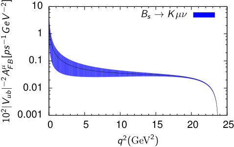 Figure 1
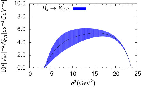 Figure 2
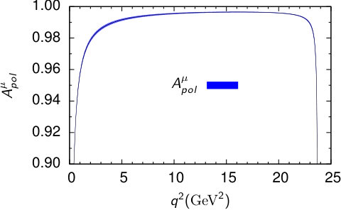 Figure 3
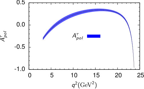 Figure 4
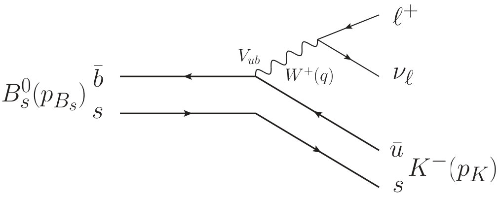 Figure 5
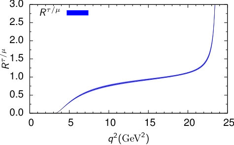 Figure 6
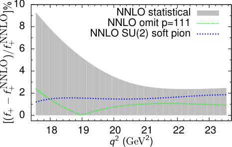 Figure 7
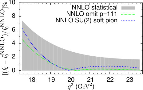 Figure 8
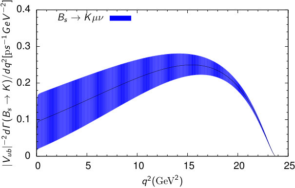 Figure 9
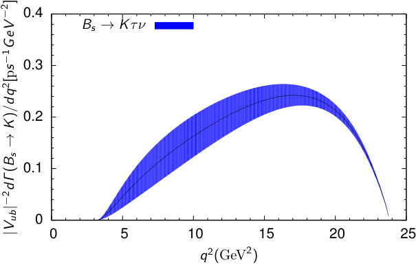 Figure 10
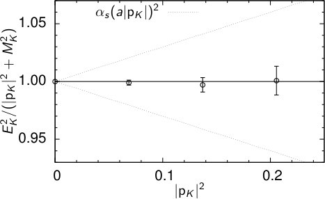 Figure 11
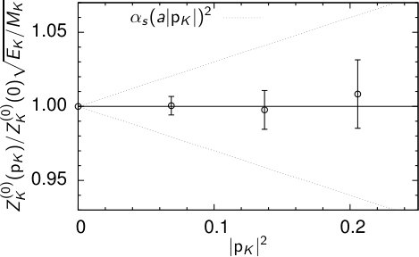 Figure 12
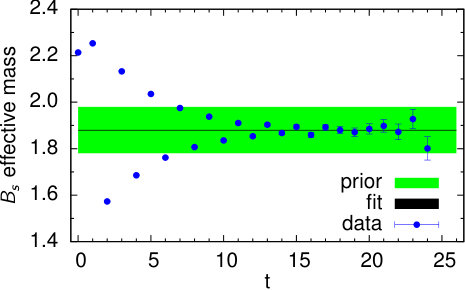 Figure 13
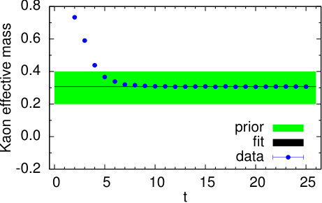 Figure 14
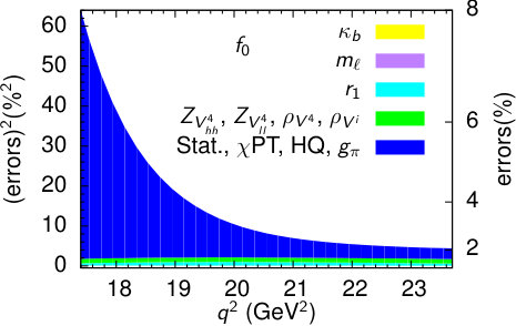 Figure 15
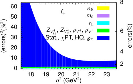 Figure 16
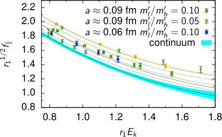 Figure 17
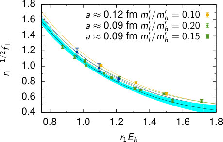 Figure 18
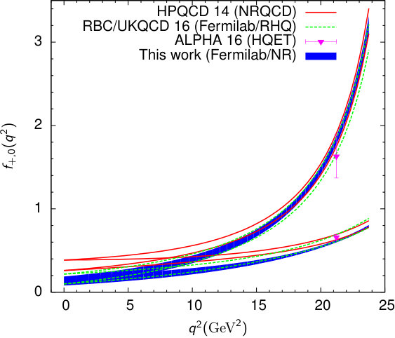 Figure 19
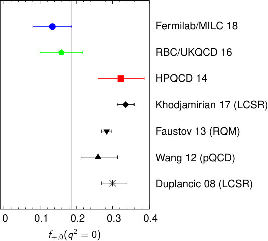 Figure 20
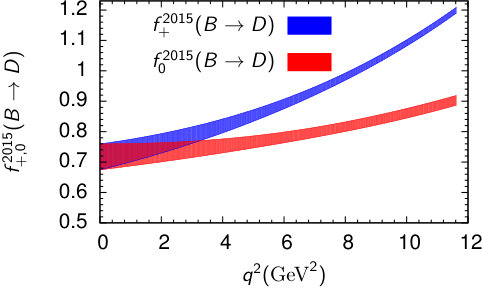 Figure 21
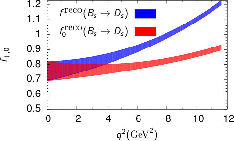 Figure 22
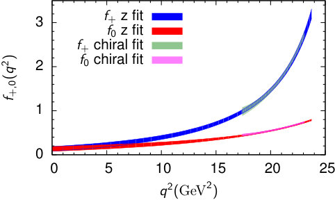 Figure 23
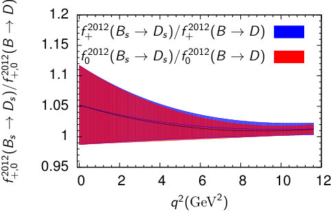 Figure 24
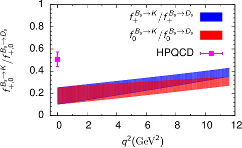 Figure 25
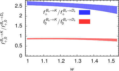 Figure 26
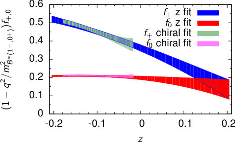 Figure 27
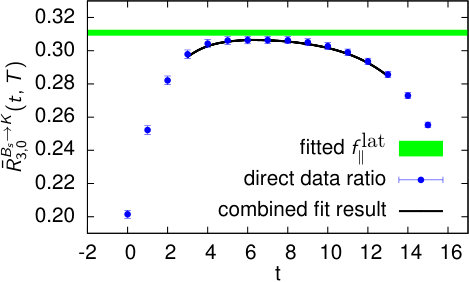 Figure 28
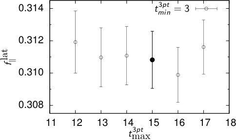 Figure 29
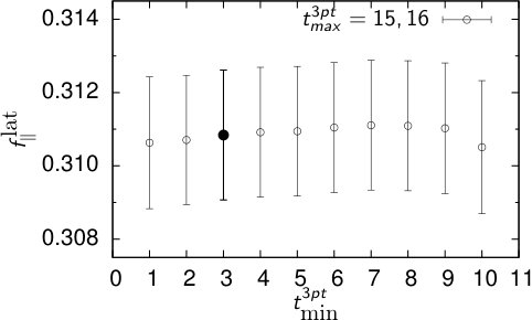 Figure 30
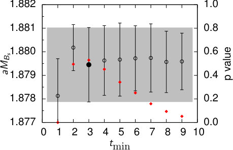 Figure 31
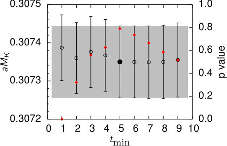 Figure 32
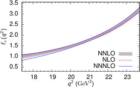 Figure 33
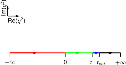 Figure 34
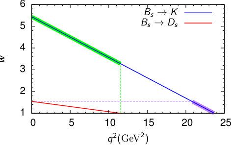 Figure 35
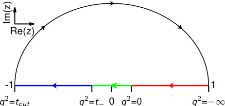 Figure 36
| a (fm) | ||||||
|---|---|---|---|---|---|---|
| 0.12 MILC Collaboration (2015a) | 0.0050/0.050 | 6.76 | 0.8678 | 2099 | 3.8 | |
| 0.09 MILC Collaboration (2015b, c, d) | 0.0062/0.031 | 7.09 | 0.8782 | 1931 | 4.1 | |
| 0.09 MILC Collaboration (2015e) | 0.00465/0.031 | 7.085 | 0.8781 | 1015 | 4.1 | |
| 0.09 MILC Collaboration (2015f, g) | 0.0031/0.031 | 7.08 | 0.8779 | 1015 | 4.2 | |
| 0.09 MILC Collaboration (2015h) | 0.00155/0.031 | 7.075 | 0.877805 | 791 | 4.8 | |
| 0.06 MILC Collaboration (2015i, j) | 0.0018/0.018 | 7.46 | 0.88764 | 827 | 4.3 |
| a (fm) | a/a | ||||
|---|---|---|---|---|---|
| 0.12 | 0.0050/0.0336 | 1.53 | 0.0901 | 0.09332 | |
| 0.09 | 0.0062/0.0247 | 1.476 | 0.0979 | 0.096765 | |
| 0.09 | 0.00465/0.0247 | 1.477 | 0.0977 | 0.096708 | |
| 0.09 | 0.0031/0.0247 | 1.478 | 0.0976 | 0.096688 | |
| 0.09 | 0.00155/0.0247 | 1.478 | 0.0976 | 0.0967 | |
| 0.06 | 0.0018/0.0177 | 1.4298 | 0.1052 | 0.0963 |
| a (fm) | (MeV) | (MeV) | ||||
|---|---|---|---|---|---|---|
| 0.12 | 2.73859 | 0.0868(9)(3) | 0.14096 | 277 | 456 | |
| 0.09 | 3.78873 | 0.0967(7)(3) | 0.139119 | 354 | 413 | |
| 0.09 | 3.77163 | 0.0966(7)(3) | 0.139134 | 307 | 374 | |
| 0.09 | 3.75459 | 0.0965(7)(3) | 0.139173 | 249 | 329 | |
| 0.09 | 3.73761 | 0.0964(7)(3) | 0.13919 | 177 | 277 | |
| 0.06 | 5.30734 | 0.1050(5)(2) | 0.137678 | 224 | 255 |
| a (fm) | |||||
|---|---|---|---|---|---|
| 0.12 | 1.7410(30) | 0.5015(8) | 0.973082 | 1.006197 | |
| 0.09 | 1.7770(50) | 0.4519(15) | 0.975822 | 0.999308 | |
| 0.09 | 1.7760(50) | 0.4530(15) | 0.975775 | 0.999405 | |
| 0.09 | 1.7760(50) | 0.4536(15) | 0.975744 | 0.999441 | |
| 0.09 | 1.7760(50) | 0.4536(15) | 0.975703 | 0.999416 | |
| 0.06 | 1.8070(70) | 0.4065(21) | 0.979176 | 0.995327 |
| a (fm) | |||
|---|---|---|---|
| 0.12 | 4 | 18 | |
| 0.09 | 4 | 25 | |
| 0.09 | 8 | 25 | |
| 0.09 | 8 | 25 | |
| 0.09 | 4 | 25 | |
| 0.06 | 4 | 36 |
| a (fm) | Kaon | meson |
|---|---|---|
| 0.12 | [5,31] | [3,22] |
| 0.09 | [7,47] | [4,30] |
| 0.06 | [10,71] | [6,44] |
| 130.4 MeV | 0.45(8) | 0(1.0) | 0(0.6) | 0(1.0) |
| Lattice data range | |||
|---|---|---|---|
| Physical range | |||
| 0.780 | 23.7 | ||
| 29.3 | |||
| 1.84 | 16.5 | 0.0 | |
| 0.102 | 28.4 | ||
| 32.3 |
| Value | 5.36682 | 0.493677 | 5.27931 | 0.1349766 | 5.32465 | 5.68 |
|---|
| Correlation matrix | |||||||||
|---|---|---|---|---|---|---|---|---|---|
| Value | |||||||||
| 0.3623(0.0178) | 1.0000 | 0.6023 | 0.0326 | -0.1288 | 0.7122 | 0.6035 | 0.5659 | 0.5516 | |
| -0.9559(0.1307) | 1.0000 | 0.4735 | 0.2677 | 0.7518 | 0.9086 | 0.9009 | 0.8903 | ||
| -0.8525(0.4783) | 1.0000 | 0.9187 | 0.5833 | 0.7367 | 0.7340 | 0.7005 | |||
| 0.2785(0.6892) | 1.0000 | 0.4355 | 0.5553 | 0.5633 | 0.5461 | ||||
| 0.1981(0.0101) | 1.0000 | 0.8667 | 0.7742 | 0.7337 | |||||
| -0.1661(0.1130) | 1.0000 | 0.9687 | 0.9359 | ||||||
| -0.6430(0.4385) | 1.0000 | 0.9899 | |||||||
| -0.3754(0.4535) | 1.0000 | ||||||||
| a (fm) | 0.12 | 0.09 | 0.06 | 0 |
| 6.831904 | 6.638563 | 6.486649 | 6.015349 | |
| 0 | 0 | 0 | 0 | |
| 0.22705 | 0.07469 | 0.02635 | 0 | |
| 0.36616 | 0.12378 | 0.04298 | 0 | |
| 0.48026 | 0.15932 | 0.05744 | 0 | |
| 0.60082 | 0.22065 | 0.07039 | 0 | |
| 0.0 | 0.0 | 0.0 | 0 | |
| 0 |
| Correlation matrix | |||||||||||||
|---|---|---|---|---|---|---|---|---|---|---|---|---|---|
| Value | 0-2 | 2-4 | 4-6 | 6-8 | 8-10 | 10-12 | 12-14 | 14-16 | 16-18 | 18-20 | 20-22 | 22-24 | |
| 0-2 | 0.20707(0.14609) | ||||||||||||
| 2-4 | 0.25741(0.14256) | ||||||||||||
| 4-6 | 0.30678(0.13329) | ||||||||||||
| 6-8 | 0.35666(0.12140) | ||||||||||||
| 8-10 | 0.40477(0.10755) | ||||||||||||
| 10-12 | 0.44785(0.09239) | ||||||||||||
| 12-14 | 0.48121(0.07653) | ||||||||||||
| 14-16 | 0.49783(0.06056) | ||||||||||||
| 16-18 | 0.48688(0.04502) | ||||||||||||
| 18-20 | 0.43098(0.03061) | ||||||||||||
| 20-22 | 0.30246(0.01787) | ||||||||||||
| 22-24 | 0.08453(0.00502) | ||||||||||||
| Correlation matrix | ||||||||||||
|---|---|---|---|---|---|---|---|---|---|---|---|---|
| Value | 2-4 | 4-6 | 6-8 | 8-10 | 10-12 | 12-14 | 14-16 | 16-18 | 18-20 | 20-22 | 22-24 | |
| 2-4 | 0.00500(0.00269) | |||||||||||
| 4-6 | 0.09085(0.04127) | |||||||||||
| 6-8 | 0.19913(0.07215) | |||||||||||
| 8-10 | 0.28718(0.08104) | |||||||||||
| 10-12 | 0.36067(0.07799) | |||||||||||
| 12-14 | 0.42097(0.06852) | |||||||||||
| 14-16 | 0.46455(0.05576) | |||||||||||
| 16-18 | 0.48267(0.04190) | |||||||||||
| 18-20 | 0.45879(0.02887) | |||||||||||
| 20-22 | 0.36241(0.01781) | |||||||||||
| 22-24 | 0.14148(0.00609) | |||||||||||
Peer Reviews
No public reviews on file for this paper yet. If you reviewed it on a platform where reviews are public (OpenReview, ICLR, NeurIPS, ICML), you can paste yours below so the community can read it here.
Videos
No videos yet. Explain this paper in a talk, walkthrough, or lecture? Add one.
Fermilab Lattice and MILC Collaborations
decay from lattice QCD
A. Bazavov
Department of Computational Mathematics, Science and Engineering,
and Department of Physics and Astronomy, Michigan State University, East Lansing, Michigan 48824, USA
C. Bernard
Department of Physics, Washington University, St. Louis, Missouri 63130, USA
C. DeTar
Department of Physics and Astronomy, University of Utah,
Salt Lake City, Utah 84112, USA
Daping Du
Department of Physics, Syracuse University, Syracuse, New York 13244, USA
A.X. El-Khadra
Department of Physics, University of Illinois, Urbana, Illinois 61801, USA
Fermi National Accelerator Laboratory, Batavia, Illinois 60510 USA
E.D. Freeland
Liberal Arts Department, School of the Art Institute of Chicago, Chicago, Illinois, USA
E. Gámiz
CAFPE and Departamento de Fisica Teórica y del Cosmos, Universidad de Granada, E-18071 Granada, Spain
Z. Gelzer
Department of Physics, University of Illinois, Urbana, Illinois 61801, USA
Steven Gottlieb
Department of Physics, Indiana University, Bloomington, Indiana 47405 USA
U.M. Heller
American Physical Society, Ridge, New York 11961, USA
A.S. Kronfeld
Fermi National Accelerator Laboratory, Batavia, Illinois 60510 USA
Institute for Advanced Study, Technische Universität München, 85748 Garching, Germany
J. Laiho
Department of Physics, Syracuse University, Syracuse, New York 13244, USA
Yuzhi Liu
Department of Physics, Indiana University, Bloomington, Indiana 47405 USA
P.B. Mackenzie
Fermi National Accelerator Laboratory, Batavia, Illinois 60510 USA
Y. Meurice
Department of Physics and Astronomy, University of Iowa,
Iowa City, IA, USA
E.T. Neil
Department of Physics, University of Colorado, Boulder, Colorado 80309, USA
RIKEN-BNL Research Center, Brookhaven National Laboratory,
Upton, New York 11973, USA
J.N. Simone
Fermi National Accelerator Laboratory, Batavia, Illinois 60510 USA
D. Toussaint
Physics Department, University of Arizona, Tucson, Arizona 85721, USA
R.S. Van de Water
Fermi National Accelerator Laboratory, Batavia, Illinois 60510 USA
Ran Zhou
Fermi National Accelerator Laboratory, Batavia, Illinois 60510 USA
Abstract
We use lattice QCD to calculate the form factors and for the semileptonic decay . Our calculation uses six MILC asqtad 2+1 flavor gauge-field ensembles with three lattice spacings. At the smallest and largest lattice spacing the light-quark sea mass is set to 1/10 the strange-quark mass. At the intermediate lattice spacing, we use four values for the light-quark sea mass ranging from 1/5 to 1/20 of the strange-quark mass. We use the asqtad improved staggered action for the light valence quarks, and the clover action with the Fermilab interpolation for the heavy valence bottom quark. We use SU(2) hard-kaon heavy-meson rooted staggered chiral perturbation theory to take the chiral-continuum limit. A functional expansion is used to extend the form factors to the full kinematic range. We present predictions for the differential decay rate for both and . We also present results for the forward-backward asymmetry, the lepton polarization asymmetry, ratios of the scalar and vector form factors for the decays and . Our results, together with future experimental measurements, can be used to determine the magnitude of the Cabibbo-Kobayashi-Maskawa matrix element .
††preprint: FERMILAB-PUB-19-005-T
Contents
-
III.3 Interpolating operators, currents, and correlation functions
-
IV.2 Extracting form factors from two- and three-point correlation functions
-
V.5 Uncertainties arising from the bottom quark mass correction
-
B.3 Dealing with the near zero eigenvalue in the covariance matrix
I Introduction
Semileptonic decays of hadrons can be used to determine elements of the Cabibbo-Kobayashi-Maskawa (CKM) matrix. However, since the quarks that participate in the underlying electroweak transition are constituents of bound states, it is necessary to understand the effects of the strong interactions on the decay. These effects are encapsulated in form factors for hadronic matrix elements of the weak currents that govern the decay. Lattice QCD has allowed us to calculate the form factors with increasing precision, making possible stringent tests of the Standard Model and the CKM paradigm. Should there be a violation of unitarity of the CKM matrix, or should two decay processes that depend on the same CKM matrix element imply different values for that CKM matrix element, we would have evidence for physics beyond the Standard Model. The decay studied here, depends on the same matrix element as the decay . Indeed, the only difference between the two decay processes is that the light spectator up () or down () quark in the latter process is replaced by a strange () quark in the case at hand. Since in lattice QCD, strange quarks generally yield smaller statistical errors and are easier to deal with computationally, a lattice calculation of the form factors for decay can enable a precise determination. This, in turn, can provide a useful test of determinations from the exclusive and processes, and, if consistent, a reduced error on (exclusive) after combination.
On the experimental side, however, while BaBar del Amo Sanchez et al. (2011); Lees et al. (2012) and Belle Ha et al. (2011); Sibidanov et al. (2013) have published precise measurements of the differential decay rate for , no such measurements exist yet for . The branching fraction of the former decay is Tanabashi et al. (2018), as it is Cabibbo suppressed compared to final states with charm. As BaBar and Belle observed many more than events, it is not surprising that experimental measurements of the latter decay have not yet been reported. In contrast, the LHCb experiment at the CERN LHC collider observes decays of all -flavored hadrons, including mesons. They are expected to publish the results of their ongoing decay study within the coming year Ciezarek et al. (2017). The Belle II experiment Urquijo (2015), where the collisions provide a cleaner environment than at the LHC, also expects to study this decay. The current plans are that Belle II will collect about at the resonance (which decays predominantly into -meson pairs), and at the , a rich source of -meson pairs Urquijo (2015). Thus, we do not expect the experimental accuracy for Belle II’s future measurement of decay rates to rival that of their expected results for , but we do expect this decay to be studied by Belle II.
This work is part of a broad study of flavor physics by the Fermilab Lattice and MILC Collaborations to determine a number of CKM matrix elements from semileptonic Bazavov et al. (2013a), Aubin et al. (2005), and Bernard et al. (2009); Bailey et al. (2009, 2012a, 2012b, 2014, 2015a, 2015b, 2015c, 2016); Du et al. (2016) decays using the asqtad flavor ensembles generated by the MILC Collaboration Bernard et al. (2001); Aubin et al. (2004); Bazavov et al. (2010a). These studies are currently being extended Bazavov et al. (2014); Gámiz et al. (2016); Primer et al. (2017); Gelzer et al. (2018a); Bazavov et al. (2018a) to use HISQ flavor ensembles Bazavov et al. (2010b, 2013b). These newer ensembles include ones with physical-mass Goldstone pions at several lattice spacings that significantly improve our control of the chiral limit. In order to provide a systematic mode by mode comparison of results obtained with the two sets of configurations, it is important to complete this analysis of .
The techniques used here are very similar to those employed in Ref. Bailey et al. (2015b), where the functional expansion was introduced. However, in this work, we use a subset of six MILC ensembles covering a range of lattice spacing between approximately 0.12 and 0.06 fm. Prior work used 12 ensembles including one with fm.
The decay has been studied by three other lattice-QCD groups, the HPQCD Collaboration Bouchard et al. (2014), the RBC and UKQCD Collaborations Flynn et al. (2015), and the ALPHA Collaboration Bahr et al. (2016), each choosing different actions for the -quark and for the light sea and valence quarks. Other previous calculations of the decay form factors are based on the relativistic quark model Faustov and Galkin (2013), light-cone sum rules Duplancic and Melic (2008); Khodjamirian and Rusov (2017), and next-to-leading-order (NLO) perturbative QCD Wang and Xiao (2012). In Sec. VI.3, we compare our results with the prior results. Preliminary reports on this study can be found in Refs. Liu et al. (2014) and Liu et al. (2018), where the vector current renormalization factors were still multiplied by a blinding factor. This factor was disclosed only after the analysis was finalized.
The rest of this paper is organized as follows. In Sec. II, we define the continuum decay form factors and the hadronic matrix elements needed to calculate them. In Sec. III, we introduce the lattice QCD operators and the form factors most convenient to calculate on the lattice. We detail how to calculate the needed lattice matrix elements and enumerate the MILC asqtad 2+1 flavor ensembles we have used. Section IV discusses our analysis of the two- and three-point functions needed to construct the lattice form factors. We also explain how we take the chiral-continuum limit. Section V contains our analysis of systematic errors in the range of momentum transfer accessible in our calculation. To construct the continuum form factors over the entire range of momentum transfer, we present the functional expansion in Sec. VI. We then apply it to obtain our final results for the form factors. Section VII presents some of the phenomenological implications of the results. Appendix A contains details of our application of SU(2) chiral perturbation theory to perform the chiral extrapolation in Sec. IV. Appendix B details how we construct the continuum form factors in Sec. VI.2. Appendix C contains the binned differential decay rates, as well as the full correlation matrices.
II Matrix elements and form factors
To lowest order in the weak coupling constant, the semileptonic decay can be described via the Feynman diagram shown in Fig. 1.
The relevant hadronic matrix element can be written as
[TABLE]
where is the vector current, and are the and four-momenta, respectively, and are the corresponding meson masses, is the momentum transferred to the lepton pair, and and are the vector and scalar form factors corresponding to the exchange of and particles. These two form factors are subject to a kinematic constraint:
[TABLE]
which eliminates the spurious pole at in Eq. (1). The tensor form factor parametrizes the hadronic matrix element of the tensor current . Since it does not contribute to the Standard Model decay rate, we do not include it in this calculation.
In the Standard Model, the angular-dependent differential decay rate for the can be written as
[TABLE]
in the meson rest frame. Here is the Fermi constant, is an element of the CKM matrix, is the lepton mass, and is the angle between the final charged-lepton and the meson momenta in the rest frame of the final state leptons. Thus, to determine from a measurement of the differential decay rate, it is necessary to compute the form factor . If the charged lepton is the , however, the lepton mass cannot be neglected and is also necessary.
III Lattice-QCD calculation
In this section, we present the ingredients of our lattice-QCD calculation. The definitions of form factors and correlation functions are given in Sec. III.1. The lattice actions and simulation parameters are described in Sec. III.2. The lattice interpolating operators, currents, and correlation functions are presented in Sec. III.3.
III.1 Definitions
For lattice calculations and Heavy Quark Effective Theory (HQET), it is convenient to work in the rest frame and introduce the four-velocity
[TABLE]
The square of the lepton momentum transfer can then be expressed as
[TABLE]
where is the kaon energy. Defining
[TABLE]
as the projection of the kaon momentum in the direction perpendicular to and using Eq. (5), one can rewrite the matrix element Eq. (1) in terms of the form factors and as
[TABLE]
The relations to the original form factors and are given by
[TABLE]
The kinematic constraint, Eq. (2), is automatically satisfied in Eq. (8).
In the rest frame, which we use throughout the lattice-QCD calculation, the form factors and are related to the temporal and spatial components of the matrix element of the vector current via
[TABLE]
Note that there is no summation over the superscript in Eq. (9b). The continuum-QCD current is related to the lattice current operator by a multiplicative renormalization factor, i.e.,
[TABLE]
The lattice current is defined in Sec. III.3, below. We use a mostly nonperturbative method to compute . The details are explained in Sec. III.3.
The desired matrix elements (and hence form factors) can be calculated from suitably defined two- and three-point correlation functions:
[TABLE]
where and are lattice interpolating operators, which are defined in Sec. III.3, below. Further, is the kaon spatial momentum, whose components in a finite volume are integer multiples of , where is the lattice spatial dimension in lattice units.
The basic procedure for calculating the continuum form factors and in Eq. (1) in lattice QCD is the following:
For each ensemble:
- (i)
Determine the lattice meson masses, kaon masses and energies from the lattice two-point correlation functions. 2. (ii)
Determine the lattice form factors and at several discrete kaon momenta from the two- and three-point correlation functions. 3. (iii)
Obtain the renormalized form factors by matching the lattice current to the continuum as in Eq. (10). 2. 2.
Use chiral perturbation theory together with Symanzik effective theory to perform a combined chiral-continuum fit to the renormalized form factors and extrapolate them to the physical quark masses and continuum (zero lattice spacing) limits. This yields the continuum form factors and as functions of the kaon recoil energy in the interval covered by the simulation, roughly GeV GeV. 3. 3.
Construct the continuum form factors and from and via Eq. (8) and employ a expansion to parametrize their shapes and to extrapolate them from the low-recoil range to the entire kinematically allowed region, which extends at high recoil to .
III.2 Actions and parameters
We use lattice gauge configurations with flavors generated by the MILC Collaboration Bazavov et al. (2010a); Bernard et al. (2001); Aubin et al. (2004). These configurations include two degenerate dynamical light quarks, acting as and quarks, and one heavier, , quark. The gluon fields are simulated with the one-loop improved Lüscher-Weisz action Lüscher and Weisz (1985). The tadpole-improved staggered action (asqtad) Blum et al. (1997); Lepage (1998); Lagaë and Sinclair (1999); Lepage (1999); Orginos and Toussaint (1999); Orginos et al. (1999); Bernard et al. (2000a) is used for generating dynamical light quarks (, , and ). Reference Bazavov et al. (2010a) is a review of simulations and formalism of improved staggered quarks.
The asqtad fermion action is also used for the valence , , and quarks. The heavy valence bottom () quarks use the Sheikholeslami-Wohlert (SW) Wilson-clover action Sheikholeslami and Wohlert (1985) with the Fermilab interpretation El-Khadra et al. (1997).
Some of the parameters used to generate the configurations are listed in Table 1. Six ensembles with three different lattice spacings, , 0.09, and 0.06 fm, are used. For each lattice spacing, we have dynamical sea quarks with light-to-strange quark mass ratio 111In this paper, we use primed quantities to denote the sea quarks and the unprimed for the valence quark.. For the intermediate lattice spacing , we have three additional values of , and 0.2 to provide results for the chiral extrapolation. The subset of ensembles used for the analysis is based on experience from previous semileptonic form factor analyses Bailey et al. (2015b) and Bailey et al. (2016). The tadpole factor appearing in the one-loop improved Lüscher-Weisz gauge action and in the asqtad fermion action are determined from the fourth root of the average plaquette.
The parameters used in the valence quarks and in generating correlation functions are listed in Table 2. The valence light quarks are degenerate with the sea quarks, i.e., ; the valence quark masses are set to our best determination of the quark mass on each ensemble, based on all of our analysis of the asqtad ensembles. In general . The heavy quark Wilson fermions with SW lattice action are controlled by the hopping parameter and the clover coefficient of the SW action . We use to denote the values used in the computation. We use the tadpole-improved tree-level value for , with listed in Table 1. The parameter is used for the correlation function generation and will be explained later in Sec. III.3.
Table 3 lists the parameters derived from the lattice simulation. The relative lattice scale is set by calculating on each ensemble, where is related to the force between static quarks, Sommer (1994); Bernard et al. (2000b). A mass-independent procedure is used to set . We use the to convert all lattice quantities to units. The physical value of is determined from : Bazavov et al. (2010a, 2012). The physical value Bailey et al. (2014), corresponding to the physical -quark mass, and the critical value , corresponding to the zero quark masses in the SW action on each ensemble, are also listed in Table 3. They will be used only for correcting the -quark masses as will be discussed in Sec. IV.3. The Goldstone pion mass and the root-mean-square (RMS) pion mass are listed in the last two columns of Table 3.
III.3 Interpolating operators, currents, and correlation functions
Here we specify the interpolating operators for the kaon and meson and the lattice vector current needed for the correlation functions in Eq. (11). For the kaon, the local pseudoscalar interpolating operator is used
[TABLE]
where is the one-component staggered fermion field.
The meson interpolating operator contains a -quark field, simulated with the improved Wilson action, and a light staggered field for the -quark Bailey et al. (2009); Wingate et al. (2003); Kawamoto and Smit (1981)
[TABLE]
where is the four-component -quark field, and is a spatial smearing function. We use two smearing functions for the meson. One is the local . The other one is the ground-state 1S wave function of the Richardson potential Bazavov et al. (2012).
The lattice vector current operator in Eqs. (10) and (11c) is defined as in Refs. Bailey et al. (2009) and Wingate et al. (2003)
[TABLE]
where the rotated -quark field , defined by
[TABLE]
removes discretization effects from the current El-Khadra et al. (1997). Here is a symmetric nearest-neighbor covariant difference operator. The coefficient , shown in Table 2, is set to its tadpole-improved tree-level value so that the lattice vector current is tree-level improved.
The renormalization constant , needed to match the lattice vector current to its continuum counterpart (see Eq. (10)), is determined using a mostly nonperturbative renormalization procedure Harada et al. (2002); El-Khadra et al. (2001):
[TABLE]
where and are the renormalization factors for the flavor-diagonal - and light-quark temporal vector currents that are calculated nonperturbatively in Ref. Bailey et al. (2015b) and listed in Table 4. The remaining flavor-off-diagonal parameters are calculated to one-loop order in perturbation theory, separately from this analysis, and also listed in Table 4. In order to reduce subjectivity in our analysis, we employed a blinding procedure in the form of a small multiplicative offset applied to the factors and known to only two of the authors. This blinding factor was subsequently disclosed and removed only after the analysis choices were finalized.
In the generation of the correlation functions defined in Eqs. (11), (12), (13), and (14), we increase statistics by repeating the calculation at source times evenly distributed in the direction. The three-point correlation functions are generated with two adjacent temporal source-sink separations: and . Both and are listed in Table 5. For the kaon recoil momenta we include the following lowest possible values: and . In practice, the largest momentum is too noisy and is excluded from the analysis.
IV Analysis
With lattice correlation functions in hand, we follow the steps outlined near the end of Sec. III.1 to determine the form factors defined there, where we make use of the spectral decomposition of the correlation functions to extract the desired parameters. The two-and three-point functions take the form Wingate et al. (2003):
[TABLE]
with
[TABLE]
The and terms in Eq. (17) arise because with our choice for the light-quark valence action the interpolating operators also generate opposite-parity (scalar) states. The overlap factors and describe the overlap of the interpolating operators with the states and , respectively, while the contain the desired matrix element.
In Sec. IV.1, we extract the meson masses, and the overlap factors and from the two-point correlation functions. We explain how the lattice form factors are extracted from the two- and three-point correlation functions in Sec. IV.2. We briefly describe the heavy -quark mass corrections in Sec. IV.3. The chiral-continuum fit function and extrapolation are described in Sec. IV.4.
IV.1 Analysis of the two-point correlation functions
The -meson masses, kaon masses, kaon energies, and and kaon overlap factors are obtained from fitting the two-point correlation functions to the functional forms in Eqs. (17a) and (17b).
As listed in Table 5, there are 4 or 8 time sources for each ensemble. The two-point correlation functions are averaged together and folded around before constructing the ensemble-averaged propagators and covariance matrix required for the two-point function fits. We use Bayesian constraints with Gaussian priors to perform fits to the correlation functions which include excited states. We vary the number of states and range of time slices included in the fits to separate excited state contributions from the desired ground state parameters and obtain reliable estimates of the uncertainties. The fit ranges are generally determined according to the following rules: is the largest value of where the fractional error in the correlation function is smaller than ; is chosen small enough to get a good handle on the excited states and to obtain a good correlated value as defined in Ref. Bazavov et al. (2016). The fit ranges for different lattice spacings are also adjusted so that the physical distances are similar. Our fit functions include the same number of opposite parity states as regular parity states. The number-of-states parameter in Eq. (17) therefore refers to a fit function with the pseudoscalar ground state plus of its radial excitations and scalar states. Our central value fits have . The prior central values for the ground state energies and overlap factors are guided by the effective mass and effective amplitude evaluated at large times . The effective mass and effective amplitude are constructed from the two-point correlation functions via
[TABLE]
Here stands for the lattice two-point correlation function for the kaon or meson. The prior central values for , , , , and are set according to Eq. (19) and the widths are set to be 0.1 or larger in lattice units. The prior central values for and are set using the energy difference between ground states and the corresponding excited states from the PDG Patrignani et al. (2016) values as a guide wherever available and the widths are set to be 0.1 or larger in lattice units. The prior central values for , , and are set using the fit results as a guide and the widths are set to be 0.1 or larger in lattice units. The prior central values for , , and are set using , , and as a guide and the widths are set to be 0.1 or larger in lattice units. Finally the prior central values for , , and are set to be 0.1 and the widths are set to be 1.0 or larger in lattice units. The prior widths in general are set to be large enough so that no bias is introduced in the fits. An example of the effective mass, prior, and fit result is shown in the left panel of Fig. 2. The corresponding kaon effective mass has smaller oscillations and much smaller errors as shown in the right panel of Fig. 2. Our fit results are stable over a range of choices and consistent with results from fits. We find that the lattice correlation functions are precise enough to determine the first excited and opposite-parity, , states. Including extra excited states better stabilizes the errors of fit posteriors.
The left panel of Fig. 3 shows an example of the stability plot for the meson. Fit intervals are chosen based on these plots and are listed in Table 6. Representative fit results for the kaon are shown in the right panel of Fig. 3.
The fit results for the kaon energies and overlap factors can be compared with the continuum relations
[TABLE]
to study momentum-dependent discretization errors. As illustrated in Fig. 4 we find that the and satisfy Eq. (20) albeit with increasing statistical errors at higher momenta. We therefore use the continuum relations for the kaon energies and factors whenever possible.
IV.2 Extracting form factors from two- and three-point correlation
functions
The form factors are related to the semileptonic matrix elements via Eq. (9), and the lattice matrix elements are contained in the three-point correlation function as in Eqs. (17c) and (18). To get the lattice form factors , we fit the two- and three-point correlation functions together. In particular, we perform combined two- and three-point correlation-function fits according to Eqs. (17) and (18) with . The three-point fit ranges are chosen to be with or . The parameters to be fitted are , , , , and . The prior central values for the -meson and kaon masses, , and are chosen as the posteriors of the two-point correlator fits. The kaon energies and are constrained according to Eq. (20). The and central values are taken to be the same size as and . The priors for are guided by the constructed ratio defined in Refs. Bailey et al. (2015b) and Bailey et al. (2016). The prior widths for the above parameters are chosen to be 0.1 or larger in lattice units. The priors for all the other are chosen to be . The ground-state energies obtained from the combined two- and three-point correlator fits are consistent with those from the two-point fits as described in Sec. IV.1.
Figure 5 shows that the fitted coming from the combined fit is in slight tension with the constructed ratio defined in Refs. Bailey et al. (2015b) and Bailey et al. (2016). This small difference comes from excited state contributions still present in the ratio but accounted for in the fit method used here. We find that they are significant at the present level of precision. Figure 6 shows an example of the stability of the fit result when varying the fit range.
In summary, the form factors and are obtained from and according to Eqs. (9) and (18c), after adding the renormalization factors as in Eq. (9).
IV.3 Heavy bottom quark mass correction
The heavy valence quark is simulated with the Sheikholeslami-Wohlert (SW) action Sheikholeslami and Wohlert (1985) with the Fermilab interpretation El-Khadra et al. (1997). The -quark mass is controlled by the hopping parameter . The hopping parameter used in the simulations differs slightly from the physical value as can be seen in Tables 2 and 3. We need to correct the form factors to account for these small shifts. A detailed description of the tuning analysis and results is provided in Appendix C of Ref. Bailey et al. (2014). We use the method described in Refs. Bailey et al. (2015b) and Bailey et al. (2016) to adjust the form factors to account for the slightly mistuned values of . The relative change in the form factors under small variations of the -quark mass can be described as
[TABLE]
where is the physical -quark kinetic mass, is the -quark mass used in the production run. The slopes were determined in Ref. Bailey et al. (2015b). The corrections to the form factors are about 0.1–1.8% on different ensembles.
IV.4 Chiral-continuum extrapolation
The lattice form factors extracted from the correlation functions as described in Sec. IV.2 are obtained at the three finite lattice spacings and unphysical light-quark masses listed in Table 1. Here we extrapolate them to the continuum limit and physical light-quark masses using SU(2) hard-kaon heavy-meson rooted staggered chiral perturbation theory (HMrSPT) Aubin and Bernard (2006, 2007). Based on previous experience with the analyses of similar processes in Refs. Bailey et al. (2015b) and Bailey et al. (2016), this best describes the data. Heavy-quark discretization effects are also taken into account in the chiral-continuum extrapolation.
We employ the HMrSPT expansion at next-to-leading order (NLO) in SU(2), leading order in , where is the -meson mass, and include next-to-next-to-leading-order (NNLO) analytic and generic discretization terms. In the SU(2) hard-kaon limit, the valence and sea -quark masses are taken to be infinitely heavy and hence dropped from the HMrSPT formula; the large kaon energy is integrated out, and its effects are absorbed into the low-energy constants (LECs). In Ref. Bailey et al. (2016), the conversion rules for and processes from SU(3) HMrSPT to SU(2) hard-kaon and hard-pion limits were derived. Here we follow the same procedure to obtain the corresponding formula for . The details are presented in Appendix A.
The NLO expression for form factors in the SU(2) hard-kaon limit that we obtain is
[TABLE]
where or , are the non-analytic contributions from the light-quark mass and lattice spacing, and the variables are dimensionless. They are defined in Eqs. (51) and (55). The leading-order factor is
[TABLE]
where is the decay constant involved, and is the coupling constant222 breaking effects renormalize the ratio; however, since it results in a overall multiplicative factor, it has been reabsorbed in the fitting coefficients.. The term takes the pole contribution into account and is determined by requiring and to have the same poles as the physical form factors and , respectively. This is reasonable because, by Eq. (8), is dominated by the contributions of , and , by the contributions of in the range considered. Using Eq. (5), one obtains the exact expression for :
[TABLE]
The vector meson (with ) has been experimentally measured Tanabashi et al. (2018) to be ; the scalar meson (with ) has not been observed experimentally, but a lattice calculation Gregory et al. (2011) estimates the mass difference between and states to be around :
[TABLE]
The vector-meson mass is below the production threshold that is involved in the decay, and the scalar-meson mass is above the threshold. The inclusion of the scalar pole and its exact location have little impact on the chiral fit results but stabilizes the form factor extrapolations.
NNLO analytic terms are included in the fits to take into account higher-order contributions. The leading heavy -quark discretization effects are also included. The expressions for the NNLO fit functions are
[TABLE]
where the heavy-quark discretization effects are modeled with . The mismatch functions are defined in the appendix of Ref. Bazavov et al. (2012). The next-to-leading-order (NLO) analytic term was defined previously in Eq. (22). A Bayesian method is used in the chiral-continuum fit. The priors are listed in Table 7. The fit results using the NNLO fit function in Eq. (26) are used as the central fit and are shown in Fig. 7.
V Systematic error estimations
The chiral-continuum extrapolated form factors are given in Sec. IV. The statistical-fit errors, which are propagated through each step of the analysis already include the effects of NNLO terms in the chiral expansion as well as light- and heavy-quark discretization. Here we discuss tests of the robustness of this error estimate to check for the presence of residual truncation effects. We also consider other sources of error not already included in our chiral-continuum fit function and construct a complete systematic error budget over the range of for which we have lattice data, .
V.1 Chiral-continuum extrapolation errors
Our central fit uses the NNLO SU(2) hard kaon HMrSPT fit function described in Eq. (26). In order to study truncation effects, we consider variations of the central fit function. We also perform fits which include fewer form factor data.
We estimate chiral truncation effects by comparing our central NNLO fit with fits using either only the NLO function, defined in Eq. (22), or a fit function that includes the complete set of next-to-NNLO (NNNLO) terms. The coefficients of the NNNLO terms are constrained with the same priors as the NNLO ones. Figure 8 shows the comparison of results for the form factor from the three fits. The corresponding results for are similar. We see that the results from the three different fits are consistent with each other over the range of where the simulation data are located. The NNNLO errors at small are larger since the data points in that region are scarce as can be seen in Fig. 7, and the fits cannot determine the higher order terms accurately. The truncation errors are well saturated in the region, and therefore it is unnecessary to add an additional systematic error.
The SU(2) hard-kaon formula is used for the central fit. To see how other choices of the HMrSPT formula affect the fits, we performed the fit with soft-kaon HMrSPT. The resulting difference is small, especially for the form factor. This can be seen in Fig. 9. Since the valence -quark masses are not equal to the sea ones, the corresponding SU(3) HMrSPT formula are extremely complicated. We therefore did not perform any trial fits with the SU(3) formula. Nevertheless, from previous experience, Bailey et al. (2015b, 2016), SU(3) HMrSPT typically does not provide a good description of the data.
Our results with kaon momentum up to are used in the central chiral fit. To check how the kaon energy range affects the results, we perform the fit omitting the data. The differences are shown in Fig. 9. Again, the difference is small especially for the form factor and also for at .
Based on the tests discussed above and visually summarized in Figs. 8 and 9, we find that the deviations between the results from the central fit and the alternative fits are smaller than the statistical error of the preferred central fit. We therefore do not assign additional systematic errors due to these sources.
V.2 Current renormalization uncertainties
The mostly nonperturbative renormalization procedure, described in Eq. (10), used to renormalize the matrix elements (and hence the form factors) requires, as inputs, the factors , , and . We estimate the error on due to the uncertainties of the nonperturbatively determined and by varying their central values by one standard deviation in each direction. As expected, the resulting changes in the form factors are small, yielding errors on in the range of 0.2–0.3%.
For and , the dominant source of error is the truncation at one-loop order in perturbation theory. As seen in Table 4, the one-loop corrections provided by and are small, with () deviating from unity by less than (). Here, we adopt the estimate of the perturbative truncation error presented in Ref. Bailey et al. (2015b), which yields an uncertainty of on both and . This estimate is consistent with the observed differences between nonperturbative Chakraborty et al. (2014) and perturbative El-Khadra et al. (2007) calculations of , discussed in Ref. Chakraborty et al. (2014). In particular, the observed differences decrease in the continuum limit, as expected. Note, however, that the nonperturbative result Chakraborty et al. (2014) employs the HISQ action for the light quarks, while our one-loop results El-Khadra et al. (2007) employ the asqtad action. For this reason, the comparison is suggestive but not definitive.
V.3 Lattice-scale uncertainties
The dimensionful form factors and , and meson energies and masses are converted to physical units via the relative scales listed in Table 3 and the absolute scale fm Bazavov et al. (2012). The statistical errors on are small and their effects on the form factors can be neglected. We estimate the error due to the uncertainty of , as before, by shifting its value by one standard deviation and repeating the chiral fit. The shifts on the form factors are at most in the range of simulated momenta.
V.4 Quark mass uncertainties
The continuum physical form factors are obtained by evaluating the chiral-continuum extrapolated functions, as discussed in Sec. IV.4 at the physical averaged - and -quark masses, namely , and the physical -quark mass as determined by analyzing the light pseudoscalar meson spectrum Bazavov et al. (2010a). The error due to the uncertainties in these masses is obtained by varying their central values by one standard deviation to find the corresponding changes in the form factors. The maximum changes are below in the simulated region.
V.5 Uncertainties arising from the bottom quark mass correction
As explained in Sec. IV.3, the form factors are adjusted to account for the slightly mistuned valence -quark masses before the chiral-continuum extrapolation. This accounts for the dominant effect from -quark mass mistuning. The errors on the form factors due to the uncertainties in the -correction factors and the tuned values are taken into account by following the procedure described in Ref. Bailey et al. (2015b). A -independent error due to tuning is assigned to both and .
V.6 Finite volume effects
Finite-volume effects, estimated by comparing infinite-volume integrals with finite sums in HMrSPT, are negligibly small Bailey et al. (2015b, 2016), so they are omitted from the total error budget.
V.7 Summary of the statistical and systematic error budgets
The systematic errors discussed in this section are summarized in Fig. 10.
We see that the largest source of systematic uncertainty by far comes from the chiral-continuum extrapolation, which includes higher-order discretization effects. This is especially obvious at small , i.e., large , because the statistical errors of the correlations functions increase with increasing recoil momentum so that the corresponding form factors at large have large errors. This is also due to a lack of data points in the large region as shown in Fig. 7. Furthermore, the HMrSPT used to perform the extrapolation is valid only for moderate . This is a generic feature common to all similar lattice calculations. Our aim, however, is to get the form factor in the whole kinematically allowed region, all the way to . In the next section, Sec. VI, we will describe how the extrapolation can be done by including physical information to control the error in the small region.
The sub-dominant errors, excluding the chiral-continuum extrapolation error, have mild dependence. Following Ref. Bailey et al. (2015b) we therefore treat them as constants in when propagating them to the -parametrization fit in Sec. VI.2. We conservatively take the maximum estimated error from each source in the simulated range and add them in quadrature. Specifically, the overall additional systematic error is 1.4% for both and , which is added to the covariance function of the chiral-continuum fit using the procedure described in Ref. Bailey et al. (2015b) prior to the next step in the analysis described in the following section.
VI Continuum form factors
The continuum form factors obtained from the chiral-continuum extrapolations described in the previous two sections are reliable only in the high momentum transfer region. In this section, we use a model-independent parametrization and expansion, namely the -parametrization, to extrapolate the form factors to the whole kinematically allowed region. This parametrization and expansion is based on the analyticity of the form factors and angular momentum conservation. The parametrization we used was introduced by Bourrely, Caprini, and Lellouch (BCL) Bourrely et al. (2009) and the fitting procedure and extrapolation technique was first introduced in our previous paper Bailey et al. (2015b).
In Sec. VI.1, we briefly review the -parametrization and give the expansion form used in the analysis. In Sec. VI.2, we present the extrapolated continuum form factors in the whole kinematically allowed region. The results are shown in Table 10, and Figs. 12 and 13. A comparison with results of other groups is presented in Sec. VI.3.
VI.1 parametrization of form factors
Before discussing the details of the method, let us first consider the properties of the semileptonic form factors. Causality and unitarity Eden et al. (1966) imply that the semileptonic form factors are real analytic functions333 An analytic function is real analytic if it satisfies . If is a real analytic function with a branch point at , then is real for and its discontinuity across the cut is purely imaginary: .
in the complex -plane with a cut from to , except at physical poles below . The parameter is the particle-pair-production threshold. For , this is
[TABLE]
The pole for the vector form factor is below the cut; while the one for the scalar form factor is above it. The above-threshold pole corresponds to an unstable particle, or resonance, and may appear only on the second Riemann sheet.
From deep-inelastic-scattering experiments and perturbative QCD scaling Lepage and Brodsky (1980); Akhoury et al. (1994), it is known that the semileptonic form factors vanish rapidly as , up to logarithmic corrections, when approaches minus infinity.
Near the threshold , the form factors have the following scaling behavior
[TABLE]
with for and for , obtained from simple partial wave analysis.
Now let us look at the parametrization. The parametrization involves a conformal mapping. Conventionally, the variable is mapped to a new variable according to
[TABLE]
where is a parameter that can be chosen to optimize the mapping. The maximum momentum transfer allowed in the semileptonic decay is defined as
[TABLE]
for convenience. This conformal mapping was first considered in Ref. Meiman (1963) and further developed and used to get model-independent constraints, usually called “unitarity bounds”, on form factors in Ref. Okubo (1971). A stronger constraint based on heavy-quark power counting was derived in Ref. Becher and Hill (2006). The conformal transformation Eq. (29) maps the physical semileptonic region onto a small region on the real axis, the upper edge of the cut onto the upper edge of the unit circle, the lower edge of the cut onto the lower edge of the unit circle, the limiting points to , and to . The complex cut plane is mapped onto the unit disk in the plane with the cut mapping onto the unit circle. The parameter can be chosen such that the semileptonic region is centered around = 0 after the conformal mapping. This is obtained by solving the equation
[TABLE]
The solution for is
[TABLE]
This mapping is schematically shown in Fig. 11 with small lepton masses ignored and with the optimized as defined in Eq. (32).
Under the above transformation, the form factors are always in the region where , and therefore they can be parametrized as a power series in . Since the physical semileptonic region in terms of is usually small, for , this parametrization converges quickly. Table 8 has a list of quantities in terms of , , and parameters.
Two commonly used parametrizations are given by Boyd, Grinstein and Lebed (BGL) Boyd et al. (1995) and by Bourrely, Caprini and Lellouch (BCL) Bourrely et al. (2009). Here we use the BCL parametrization as given by
[TABLE]
The factors take the poles into account and ensure the asymptotic scaling, at large . Moreover, the scaling condition of Eq. (28) near is also enforced for . Note that Eq. (28) in the -plane imply the following relation
[TABLE]
The form factors constructed with this BCL parametrization satisfy all three properties of the semileptonic form factors discussed at the beginning of this section.
VI.2 -parametrization fit and extrapolation
We use Eq. (33) to perform the -parametrization fit to our chiral-continuum-extrapolated form factor results obtained in Secs. IV.4 and V. The vector pole is taken to be Tanabashi et al. (2018), and the above threshold scalar pole is taken to be the theoretically predicted value Gregory et al. (2011). The parameter is chosen as in Eq. (32), and the corresponding value for the process is . Table 9 lists the relevant meson masses used in the -parametrization fit.
The functional method introduced in Ref. Bailey et al. (2015b) is used to perform the -parametrization fit, where, following Ref. Bailey et al. (2015b), we take as inputs the results from the chiral-continuum extrapolation and systematic error analysis as presented in Sec. V.7).
Our preferred (central) fit has , where is the number of terms in the expansion in Eq. (33). The results of this fit are shown in Table 10. These can be used to reconstruct the final form factors as described in Appendix B. We arrive at this preferred fit choice by first simultaneously fitting the form factors and with and without constraining the -parametrization parameters in Eq. (33). The coefficients and are well determined, but the quality of this fit is poor. When increasing from 2 to 3, the quality of the fit improves, and all the coefficients can be determined well. The kinematic constraint Eq. (2) is satisfied within errors444Note that the kinematic constraint is automatically satisfied in Eq. (8) before taking the extrapolation as is being done in this section. After the extrapolation, this constraint is not guaranteed if not imposed in the fit.. Enforcing this kinematic constraint, as explained below, further improve the form-factor fit. The fit parameters also satisfy the unitarity condition Bourrely et al. (2009) and the condition estimated from heavy-quark power counting Becher and Hill (2006). Adding the heavy-quark constraint does not affect the fit results. The kinematic constraint is enforced by requiring and to be exactly equal at the point. In practice, we set a prior in the -parametrization fit
[TABLE]
with width . When further increasing the expansion order to , the central value of the form factors at agrees with the results with , but the error increases. The unitarity and heavy-quark constraints are still satisfied automatically. The results stabilize at and do not change with . We conclude that the fit with the kinematic constraint includes the systematic uncertainty due to truncating the -parametrization series.
The left panel of Fig. 12 shows the preferred form-factor results, with poles removed, as functions of . The point is at the right end of the plot. Note that the shape of the form factors as functions of is parametrization dependent. For convenience, the right panel of Fig. 12 shows the form factors as functions of . The dependence of the form factors is parametrization independent and can be used directly to compare with results of other groups.
VI.3 Comparison with existing results
Several other groups have also calculated the same form factors. We note that Refs. Bouchard et al. (2014) and Flynn et al. (2015) use the threshold instead of in their implementation of the parametrization. Since the -parameter, by definition (see Eq. (29)), depends on the threshold (), we cannot directly compare the -dependence of our form factors with those of Refs. Bouchard et al. (2014) and Flynn et al. (2015). We therefore compare our form factors with those from other lattice QCD calculations only as functions of . This is shown in Figure 13.
The results of the HPQCD Collaboration Bouchard et al. (2014) are based on (2+1)-flavor-MILC-asqtad configurations for the sea quarks, and employ the HISQ action for the light valence quarks, and lattice NRQCD for the heavy -quark. The RBC and UKQCD Collaborations Flynn et al. (2015) use (2+1)-flavor-domain-wall fermions for the sea quarks and light valence quarks, and a variant Lin and Christ (2007); Christ et al. (2007) of the Fermilab action for the heavy -quark. The ALPHA Collaboration Bahr et al. (2016) uses leading-order lattice HQET to get the form factors at one point, . While our results are consistent with those from Refs. Flynn et al. (2015) and Bahr et al. (2016), they are in tension with HPQCD’s results Bouchard et al. (2014). We note that Ref. Bouchard et al. (2014) employs the so-called modified -expansion, where the chiral-continuum extrapolation is combined with the -expansion into one fit function by modifying the -coefficients with lattice-spacing and light-quark-mass dependent terms. This procedure may affect the shape of the form factors. Indeed, in their calculation of the form factors for the decay in Ref. Bouchard et al. (2013), the HPQCD Collaboration compared the form factors obtained after the modified -expansion with the results from a two-step method that is very similar to ours, performing first a chiral-continuum extrapolation, and then a -expansion fit. While they find only small differences between the two sets of form factors, those obtained from their implementation of the two-step method are in better agreement with the results of Ref. Bailey et al. (2016). However, unlike the case at hand, the form factors of Ref. Bailey et al. (2016) are not in significant tension with HPQCD’s results of Ref. Bouchard et al. (2013). We see that the tension between our form factor results and those of Ref. Bouchard et al. (2014) increases with decreasing to roughly 2.3 at . The RBC and UKQCD Collaborations Flynn et al. (2015), on the other hand, adopt the same procedure as we do, namely a chiral-continuum extrapolation at high , followed by a -expansion extrapolation to .
A comparison of the form factor at is shown in Fig. 14, where we also include results from calculations using light-cone sum rules Duplancic and Melic (2008); Khodjamirian and Rusov (2017), a relativistic quark model Faustov and Galkin (2013), and NLO perturbative QCD Wang and Xiao (2012).
VII Phenomenological applications
The angular-dependent differential decay rate for is given in Eq. (3). One can construct at most three independent observables from there. In the following, we will consider the differential decay rate in Sec. VII.1, the forward-backward asymmetry in Sec. VII.2, and the lepton polarization asymmetry in Sec. VII.3. The latter two quantities are sensitive to the mass of the final-state charged lepton. In Sec. VII.4, we also construct the ratios of the scalar and vector form factors between the and decays.
VII.1 Decay rate
The differential decay rate can be obtained from Eq. (3) by integrating over the angle , which yields
[TABLE]
In Fig. 15, we plot the Standard Model predictions of the differential decay rate divided by over the whole kinematic range of for and .
One can also explore the ratio of the differential decay rates
[TABLE]
Figure 16 shows the prediction for .
The total decay rate is given by
[TABLE]
with , as in Eq. (30). The numerical results for are
[TABLE]
In Appendix C, we also provide partially integrated differential decay rates in evenly spaced bins.
The ratio of the total decay rate is
[TABLE]
which takes the correlations between the form factors into account and is more precise than directly using Eq. (39).
VII.2 Forward-backward asymmetry
The forward-backward asymmetry, , which depends on the linear term in Eq. (3), is given by
[TABLE]
The Standard Model predictions for the forward-backward asymmetry divided by are shown in Fig. 17.
For the corresponding integrated quantities we find
[TABLE]
The normalized forward-backward asymmetry is given by
[TABLE]
and the corresponding numerical values are
[TABLE]
VII.3 Lepton polarization asymmetry
The normalized lepton polarization asymmetry is defined as
[TABLE]
from the differential decay rates with definite lepton helicity Meiß ner and Wang (2014)
[TABLE]
Here the superscripts () imply a right- (left-)handed lepton in the final state. The lepton is produced via the current in the Standard Model, and therefore the electron and muon are mainly left-handed polarized. The is close to one in the whole range. Here we provide the normalized lepton polarization asymmetry and as functions of in Fig. 18.
VII.4 Ratio of the and
form factors
We also calculate the ratios of the scalar and vector form factors between the and semileptonic decays. The ratios can be used along with future experimental results to determine the ratio of the CKM matrix elements .
First, we reconstruct the form factors from our previous papers Bailey et al. (2012b, 2015a). Form factor ratios, , and the form factors, , are calculated in Refs. Bailey et al. (2012b) and Bailey et al. (2015a), respectively. They are shown in Fig. 19.
The form factor can be reconstructed via
[TABLE]
With the reconstructed form factors shown in Fig. 20, we obtain the form-factor ratios, , shown in Fig. 21 as functions of and in Fig. 22 as functions of . Although the 2012 analysis was carried out on a subset of the ensembles used in the 2015 analysis, we neglect any correlations in the two form factors in Eq. (47). Here is the usual square of the lepton momentum transfer as defined in Eq. (5). The recoil parameter for is defined as
[TABLE]
and the corresponding one for the is defined by replacing with . The relation between and in Eq. (48), and the kinematically allowed regions for the two types of processes are shown in Fig. 23. The ratios constructed with different parameters and as shown in Figs. 21 and 22 allow us to probe the different form factor regions.
VIII Summary and Outlook
Using six strategically selected ensembles of MILC asqtad 2+1 flavor gauge configurations, we have calculated the form factors and needed to understand the semileptonic decay . We present predictions of the differential decay rate (divided by ) for both light ( or ) or heavy () final-state leptons. Once the experimental data become available, our form factors can be used to determine , which can then be compared to and, if consistent, combined with the determinations from other exclusive decay processes. Hence they may help shed light on the discrepancy with from inclusive decays and, perhaps, contribute to evidence for new physics beyond the Standard Model by enabling more stringent tests of the CKM paradigm. Other quantities of phenomenological interest include the forward-backward asymmetry and the lepton polarization asymmetry . We also present ratios of the form factors and for and as functions of both and . These may be valuable for determining .
Although there are no published results for the decay , this process is under investigation by the LHCb experiment, and will be studied by the Belle II Collaboration when they run at the resonance, which is a copious source of and mesons.
On the theoretical side, we have plans to reduce the contributions from the dominant sources of systematic errors in upcoming calculations, which include chiral extrapolation, light and heavy-quark discretization, and renormalization. The gauge ensembles generated by the MILC collaboration with four flavors of HISQ sea quarks Bazavov et al. (2010b, 2013b) are a crucial ingredient in these plans. These ensembles cover a lattice spacing range of approximately 0.15–0.045 fm with physical light quark masses and a dynamical charm quark. The chiral extrapolation becomes a chiral interpolation, and the reduced taste breaking of the HISQ action greatly reduces light quark discretization errors. Using these ensembles, we will be taking two approaches to the quark. First, we have started a project using Fermilab quarks (as in this project) and HISQ light valence quarks. Preliminary results were already reported in Refs. Gelzer et al. (2018a) and Gelzer et al. (2018b). As a further small improvement compared to this work, we will include the full correlation matrix between form factors for different processes in our final results. In our second approach, we plan to use the HISQ formalism for the quark to calculate semileptonic - and -meson decay form factors again on the HISQ ensembles. Heavy-quark discretization errors are simpler with the HISQ action than with the Fermilab approach, and can be controlled with high precision by including ensembles with very fine lattice spacings in the range of fm. The heavy-HISQ approach also allows us to take advantage of Ward identities when renormalizing the currents. Indeed, our recent work Bazavov et al. (2018b) employing the heavy HISQ method for the - and -meson decay constants has reached unprecedented precision. We have recently started to generate the correlation functions for this project. In summary, with the improvements outlined above, we expect, in the coming years, to obtain the form factors for (and related decays) with percent level precision, at least in the low recoil region of the phase space.
Acknowledgements.
We thank Jon A. Bailey for participating in the early stage of the project. We thank Chris M. Bouchard for discussions and comments on the form factor comparison section. We thank members of the LHCb Collaboration for discussions and in particular Svende Braun, Marta Calvi, and Mika A. Vesterinen for sharing with us their analysis status and the preferred bins. Computations for this work were carried out with resources provided by the USQCD Collaboration, the National Energy Research Scientific Computing Center, the Argonne Leadership Computing Facility, the Blue Waters sustained-petascale computing project, the National Institute for Computational Science, the National Center for Atmospheric Research, the Texas Advanced Computing Center, and Big Red II+ at Indiana University. USQCD resources are acquired and operated thanks to funding from the Office of Science of the U.S. Department of Energy. The National Energy Research Scientific Computing Center is a DOE Office of Science User Facility supported by the Office of Science of the U.S. Department of Energy under Contract No. DE-AC02-05CH11231. An award of computer time was provided by the Innovative and Novel Computational Impact on Theory and Experiment (INCITE) program. This research used resources of the Argonne Leadership Computing Facility, which is a DOE Office of Science User Facility supported under Contract DE-AC02-06CH11357. The Blue Waters sustained-petascale computing project is supported by the National Science Foundation (awards OCI-0725070 and ACI-1238993) and the State of Illinois. Blue Waters is a joint effort of the University of Illinois at Urbana-Champaign and its National Center for Supercomputing Applications. This work is also part of the “Lattice QCD on Blue Waters” and “High Energy Physics on Blue Waters” PRAC allocations supported by the National Science Foundation (award numbers 0832315 and 1615006). This work used the Extreme Science and Engineering Discovery Environment (XSEDE), which is supported by National Science Foundation grant number ACI-1548562 Towns et al. (2014). Allocations under the Teragrid and XSEDE programs included resources at the National Institute for Computational Sciences (NICS) at the Oak Ridge National Laboratory Computer Center, The Texas Advanced Computing Center and the National Center for Atmospheric Research, all under NSF teragrid allocation TG-MCA93S002. Computer time at the National Center for Atmospheric Research was provided by NSF MRI Grant CNS-0421498, NSF MRI Grant CNS-0420873, NSF MRI Grant CNS-0420985, NSF sponsorship of the National Center for Atmospheric Research, the University of Colorado, and a grant from the IBM Shared University Research (SUR) program. Computing at Indiana University is supported by Lilly Endowment, Inc., through its support for the Indiana University Pervasive Technology Institute. This project was supported in part by the URA Visitig Scholar Award 12-S-15 (Y.L.); by the U.S. Department of Energy under grants No. DE-FG02-91ER40628 (C.B.), No. DE-FC02-12ER41879 (C.D.), No. DE-FG02-13ER42001 (A.X.K.), No. DE-SC0015655 (A.X.K., Z.G.), No. DE-SC0010120 (S.G.), No. DE-FG02-91ER40661 (S.G.), No. DE-SC0010113 (Y.M.), No. DE-SC0010005 (E.T.N.), No. DE-FG02-13ER41976 (D.T.); by the U.S. National Science Foundation under grants PHY14-14614 and PHY17-19626 (C.D.), and PHY14-17805 (J.L.); by the MINECO (Spain) under grants FPA2013-47836-C-1-P and FPA2016-78220-C3-3-P (E.G.); by the Junta de Andalucía (Spain) under grant No. FQM-101 (E.G.); by the Fermilab Distinguished Scholars program (A.X.K.); by the German Excellence Initiative and the European Union Seventh Framework Program under grant agreement No. 291763 as well as the European Union’s Marie Curie COFUND program (A.S.K.). Brookhaven National Laboratory is supported by the United States Department of Energy, Office of Science, Office of High Energy Physics, under Contract No. DE-SC0012704. This document was prepared by the Fermilab Lattice and MILC Collaborations using the resources of the Fermi National Accelerator Laboratory (Fermilab), a U.S. Department of Energy, Office of Science, HEP User Facility. Fermilab is managed by Fermi Research Alliance, LLC (FRA), acting under Contract No. DE-AC02-07CH11359.
Appendix A form factors in SU(2) chiral
perturbation theory
In this appendix, we derive Eq. (22), the SU(2) chiral formula for .
We start from the next-to-leading order (NLO) SU(3) HMrSPT expression for semileptonic decay. It is expressed as Aubin and Bernard (2007)
[TABLE]
where the subscript stands for or ; are coefficients and the corresponding rescaled quantities in Eq. (55) will be determined by the chiral fits; contains the one-loop nonanalytic contributions and wave-function renormalizations; and are the corresponding valence quark masses; , and are sea quark masses; is the meson energy in the meson rest frame; and is the lattice spacing. The leading order terms for and are
[TABLE]
where is the decay constant involved; is the coupling constant; is the mass difference between the quantum number or meson and the pseudoscalar meson masses at leading order in the chiral expansion, i.e., ; and is the nonanalytic self-energy contribution. The scalar pole was not included in Ref. Aubin and Bernard (2007) as the meson is not in leading order HMrSPT. It is added here phenomenologically as explained in Sec. IV.4.
For the analysis considered here, and . Here we use primed quantities to denote the valence quarks and the unprimed for the sea quarks555This is different from the convention used in the main text. For example, in Tables 1 and 2 the prime quantities denote the sea quarks and the unprimed for the valence ones.. All the data generated for analysis are partially quenched points, i.e., .
In the SU(2) limit, the -quark mass is treated as infinitely heavy and all the explicit dependent terms are removed from the formula. However, one will still need to keep the mass difference, , in the leading-order analytic term to take the partial quenching effects into account. In the hard-kaon limit, the kaon with a large energy, , is integrated out in the nonanalytic chiral expressions. These two limits greatly simplify the expressions of the chiral logs. Following the recipes presented in the Appendix of Ref. Bailey et al. (2016), we obtain the SU(2) hard-kaon chiral log terms in and for the as
[TABLE]
The summation is over 16 staggered fermion tastes (P, V, T, A, or I); is the chiral logarithm defined as
[TABLE]
Meson masses for the 2+1 case in the SU(2) limit ( and ) are Aubin and Bernard (2003); Bailey et al. (2016)
[TABLE]
The in Eq. (51) stands for terms with subscripts changed from V to A. The hairpin parameters in Eq. (53b) are listed in Table 11. The are defined later in Eq. (56).
We can regroup relevant terms in Eq. (49), drop the dependent term due to the SU(2) limit, and write the formula as the following
[TABLE]
We can further write all the expansion parameters in terms of dimensionless ones
[TABLE]
where is the leading-order low-energy constant that relates the tree-level mass of a taste- meson composed of quarks of flavor and to the corresponding quark masses
[TABLE]
Here is the staggered fermion taste splitting. The numerical values of and are determined by the MILC Collaboration and are shown in Table 11. The average taste splitting in Eq. (55d) is .
Combining the above information, one arrives at the final NLO form used in the chiral-continuum extrapolation in this work, Eq. (22).
Appendix B Reconstructing the form factors
In this appendix, we document the procedure of reconstructing the form factors from the fitting results obtained in Sec. VI.2.
B.1 Reconstructing the form factors as functions of
The form factors are parametrized in a BCL Bourrely et al. (2009) form with coefficients as shown in Eq. (33). The meson masses used in the -parametrization fit are listed in Table 9. The fitted coefficients are listed in Table 10. To get the form factors as functions of and reproduce the left panel result of Fig. 12, one should use Eq. (33) with and meson mass values in Table 9, and the values and the correlation matrix in Table 10.
B.2 Reconstructing the form factors as functions of
To get the dependence of the form factors as in the right panel of Fig. 12, one needs the relation between and . In this paper, the mapping is defined in Eqs. (29), (27), (30), and (32). One can then solve Eq. (29) to get in terms of :
[TABLE]
Once we have the form factors as functions of from Appendix B.1, we can then use Eq. (57) to change the variable to get the dependence.
B.3 Dealing with the near zero eigenvalue in the covariance matrix
In Table 10 the fit parameter standard deviations and the correlation matrix are listed. To get the covariance matrix, one only needs to follow the usual procedure to rescale the correlation matrix. The following is the detailed procedure.
Suppose the standard deviation of the fit parameters is
[TABLE]
and the matrix is a diagonal matrix with diagonal elements . The correlation matrix is denoted as and the covariance matrix is denoted as . The relations among , , and are
[TABLE]
Alternatively, one can use the following relation to directly convert the matrix elements
[TABLE]
where there is no summation over the repeated indices. The covariance matrix, or the inverse of it, is useful when combining form factor results from different sources. It is difficult to calculate the inverse of the covariance matrix from the results listed in Table 10. This is because we imposed the kinematical constraint Eq. (35) with in the -parametrization fit. This results in a near zero eigenvalue in the covariance matrix. The kinematic constraint is equivalent to reducing one parameter in the parametrization. In principle, one can first reduce one parameter, say , in Eq. (33), express it in terms of the other parameters, and then perform the -parametrization fit. This, however, will make the expression Eq. (33b) cumbersomely complicated to handle when performing the fit. In practice, we use the expressions Eq. (33) and perform the fits as described in Sec. VI.2. Whenever one needs to invert the covariance matrix, one simply needs to reduce the size of the matrix by removing one column and one row corresponding to one parameter . The parameter can be any one of the parameters. Without loss of generality, let us pick to be for our preferred fit. From Eqs. (33 and 35), we can get
[TABLE]
with
[TABLE]
as derived from Eq. (29).
Appendix C differential decay rate bin
tables
In this appendix, we present the quantity
[TABLE]
for the and decays, in bins of , in Tables 12 and 13. Since we also include the correlations between bins in these tables, the results therein can be combined with the corresponding experimental measurements to determine .
[FIGURE:]
[FIGURE:]
The reference list from the paper itself. Each links out to its DOI / PubMed record.
- 1del Amo Sanchez et al. (2011) P. del Amo Sanchez et al. (Ba Bar), Phys. Rev. D 83 , 032007 (2011) , ar Xiv:1005.3288 [hep-ex] . · doi ↗
- 2Lees et al. (2012) J. P. Lees et al. (Ba Bar), Phys. Rev. D 86 , 092004 (2012) , ar Xiv:1208.1253 [hep-ex] . · doi ↗
- 3Ha et al. (2011) H. Ha et al. (Belle), Phys. Rev. D 83 , 071101 (2011) , ar Xiv:1012.0090 [hep-ex] . · doi ↗
- 4Sibidanov et al. (2013) A. Sibidanov et al. (Belle), Phys. Rev. D 88 , 032005 (2013) , ar Xiv:1306.2781 [hep-ex] . · doi ↗
- 5Tanabashi et al. (2018) M. Tanabashi et al. (Particle Data Group), Phys. Rev. D 98 , 030001 (2018) . · doi ↗
- 6Ciezarek et al. (2017) G. Ciezarek, A. Lupato, M. Rotondo, and M. Vesterinen, JHEP 02 , 021 (2017) , ar Xiv:1611.08522 [hep-ex] . · doi ↗
- 7Urquijo (2015) P. Urquijo, Nucl. Part. Phys. Proc. 263-264 , 15 (2015) . · doi ↗
- 8Bazavov et al. (2013 a) A. Bazavov et al. (Fermilab Lattice, MILC), Phys. Rev. D 87 , 073012 (2013 a) , ar Xiv:1212.4993 [hep-lat] . · doi ↗