Modeling Magnetic Fields with Helical Solutions to Laplace's Equation
Brian Pollack, Ryan Pellico, Cole Kampa, Henry Glass, Michael Schmitt

TL;DR
This paper develops a series solution to Laplace's equation in helical coordinates, enabling precise modeling of solenoidal magnetic fields with minimal data and high accuracy, capturing complex helical features.
Contribution
It introduces a novel series solution in helical coordinates and demonstrates its effectiveness for accurate magnetic field modeling with sparse data.
Findings
Achieves better than one part per million accuracy in magnetic field modeling.
Effectively captures helical features from solenoid winding.
Uses minimal parameters and data for high-precision modeling.
Abstract
The series solution to Laplace's equation in a helical coordinate system is derived and refined using symmetry and chirality arguments. These functions and their more commonplace counterparts are used to model solenoidal magnetic fields via linear, multidimensional curve-fitting. A judicious choice of functional forms, a small number of free parameters and sparse input data can lead to highly accurate, fine-grained modeling of solenoidal magnetic fields, including helical features arising from the winding of the solenoid, with overall field accuracy at better than one part per million.
Click any figure to enlarge with its caption.
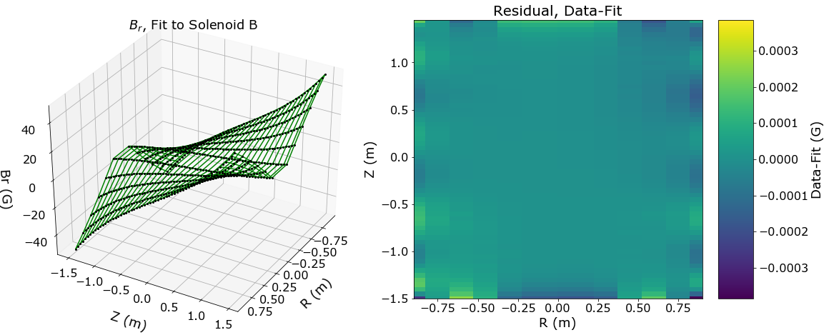 Figure 1
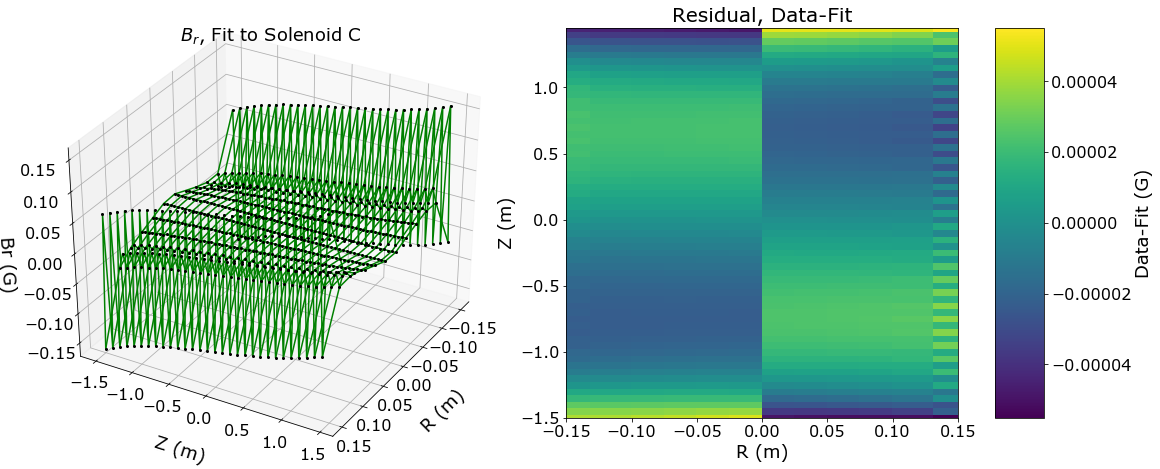 Figure 2
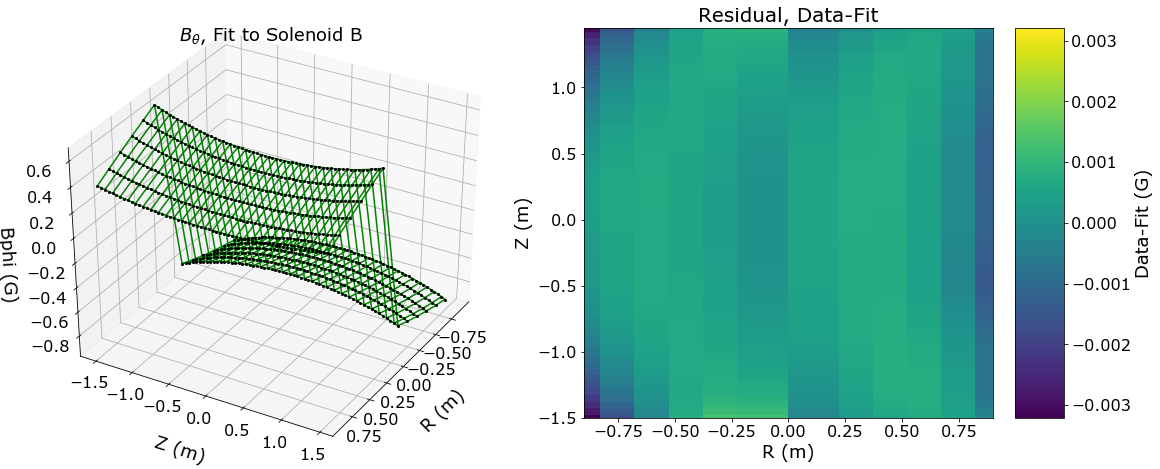 Figure 3
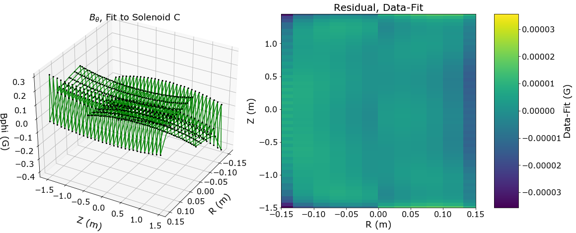 Figure 4
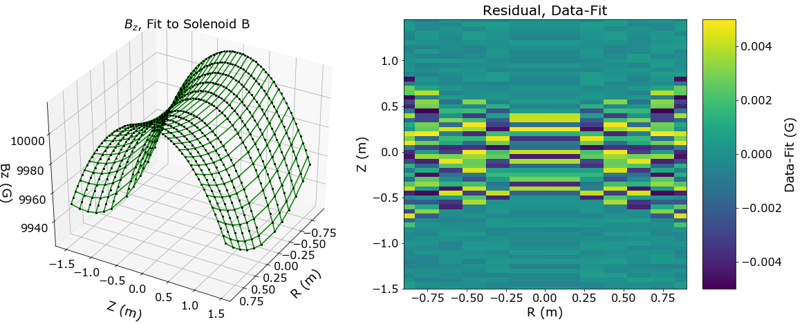 Figure 5
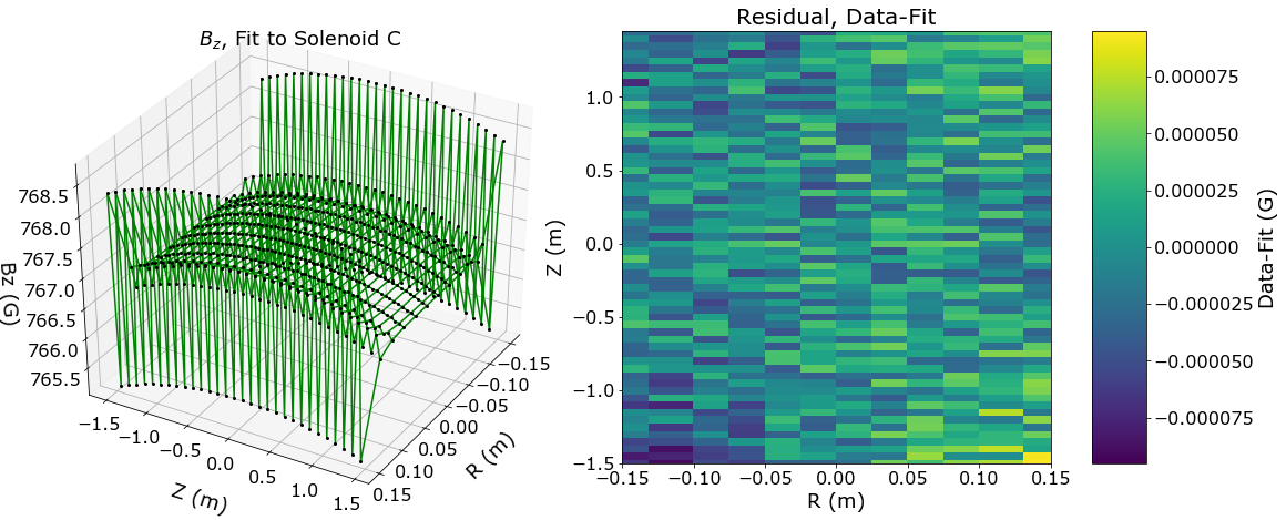 Figure 6
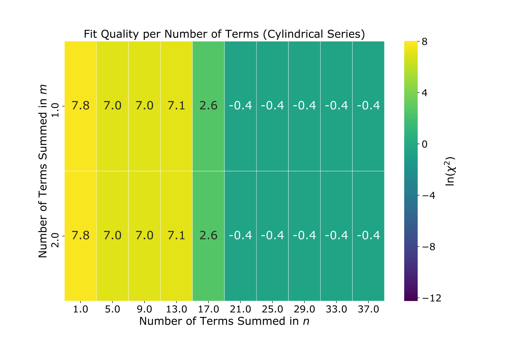 Figure 7
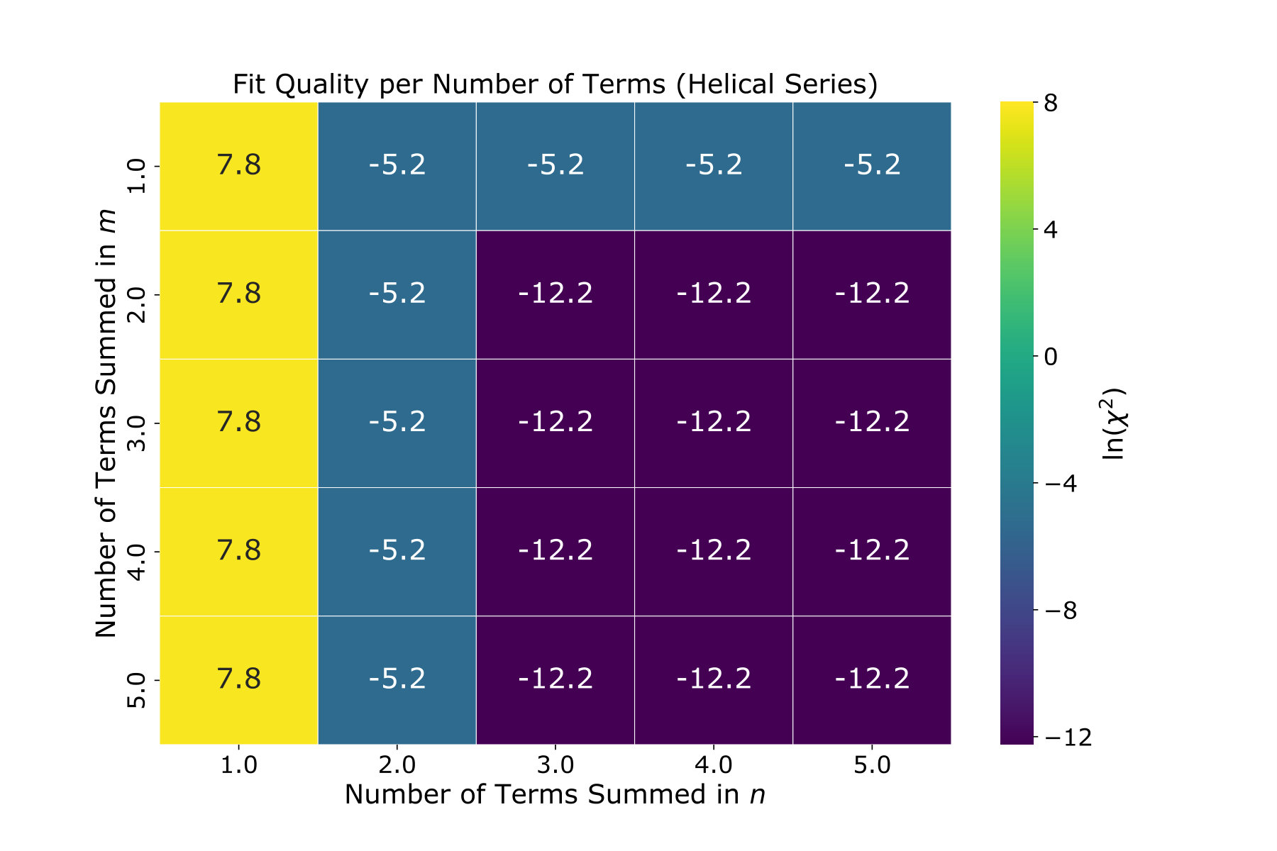 Figure 8
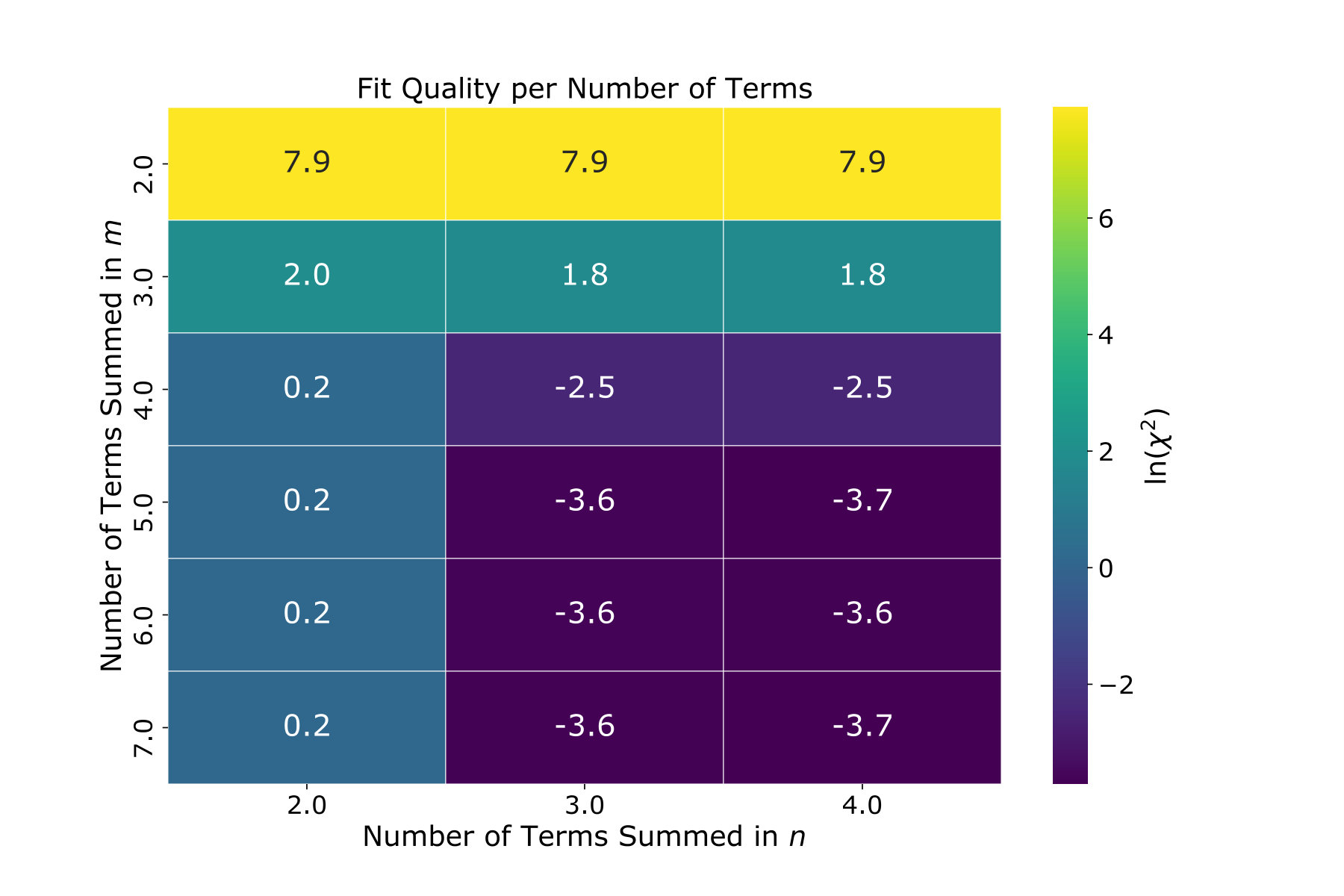 Figure 9
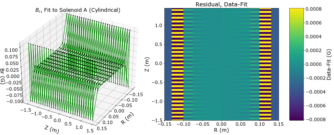 Figure 10
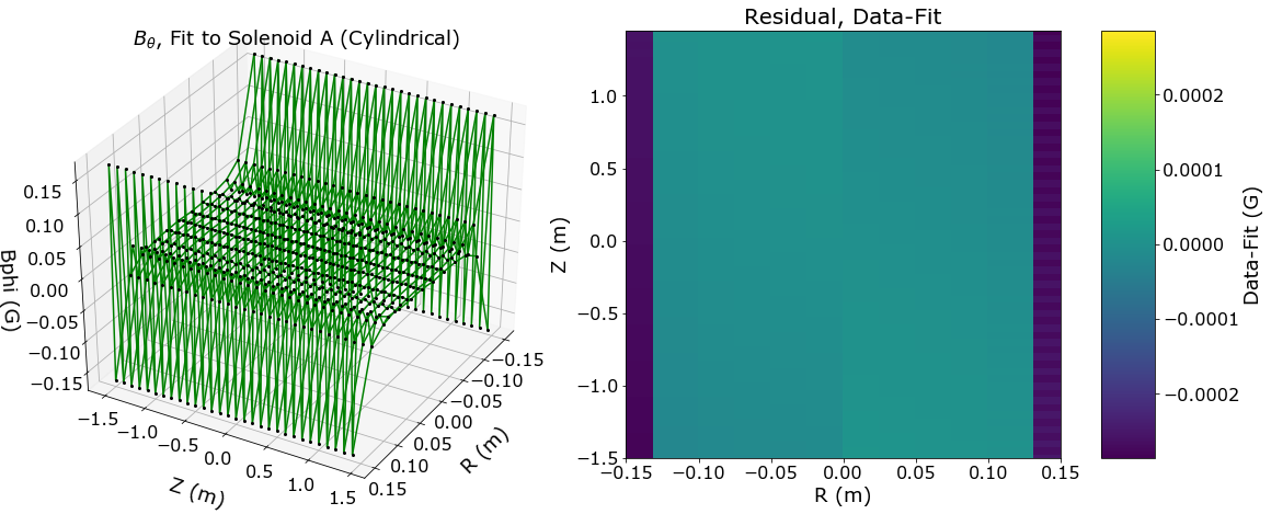 Figure 11
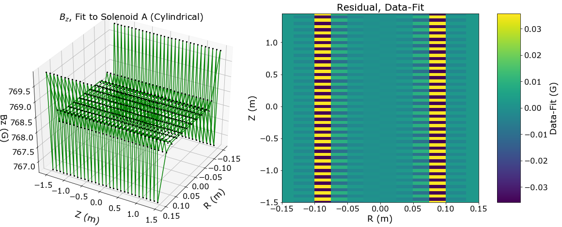 Figure 12
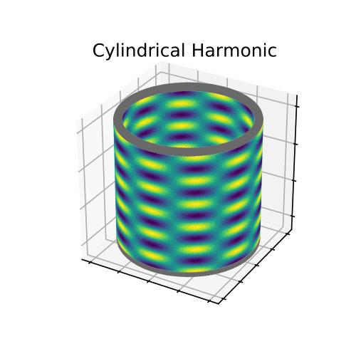 Figure 13
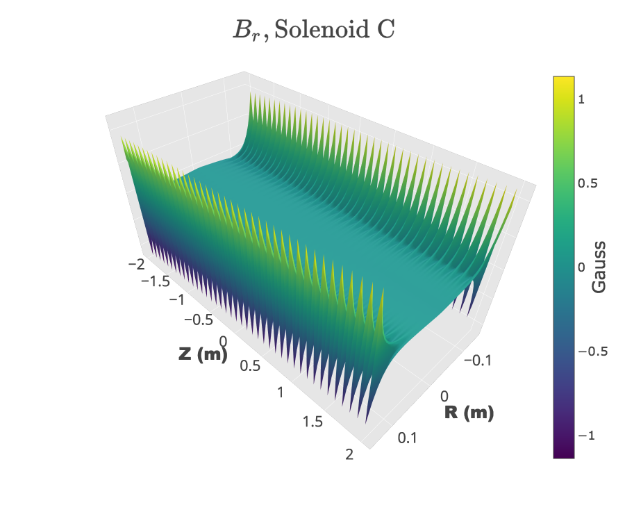 Figure 14
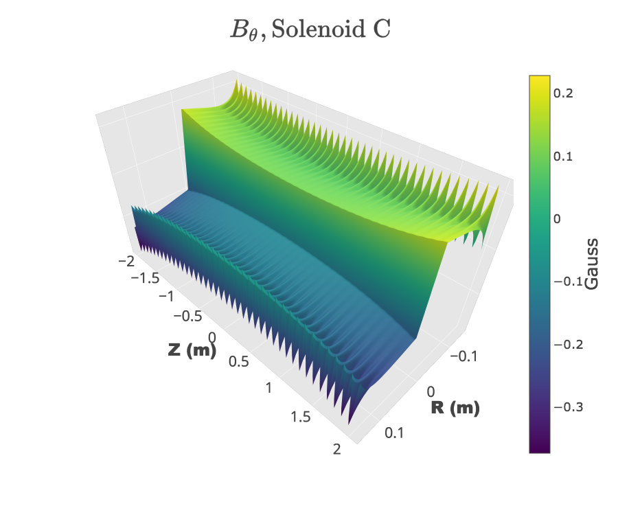 Figure 15
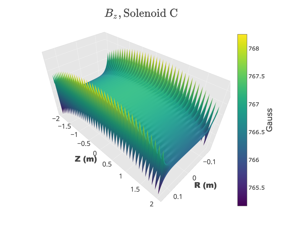 Figure 16
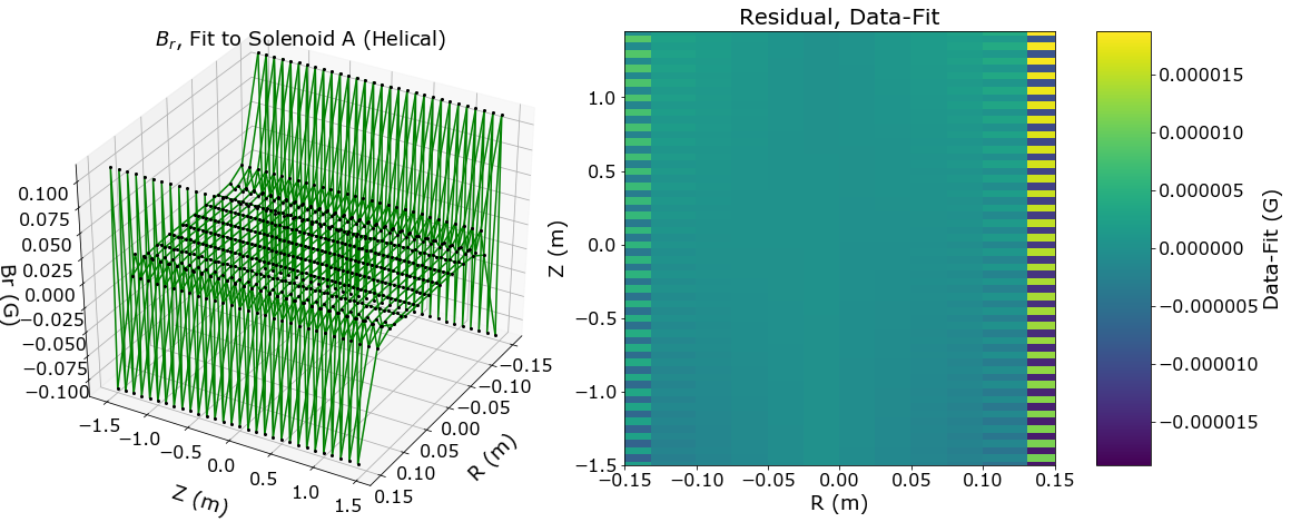 Figure 17
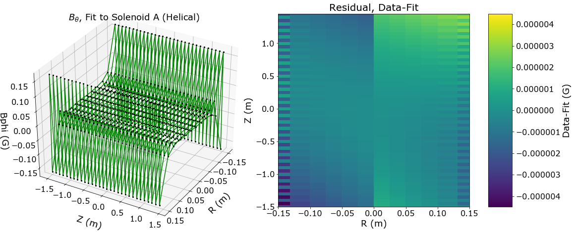 Figure 18
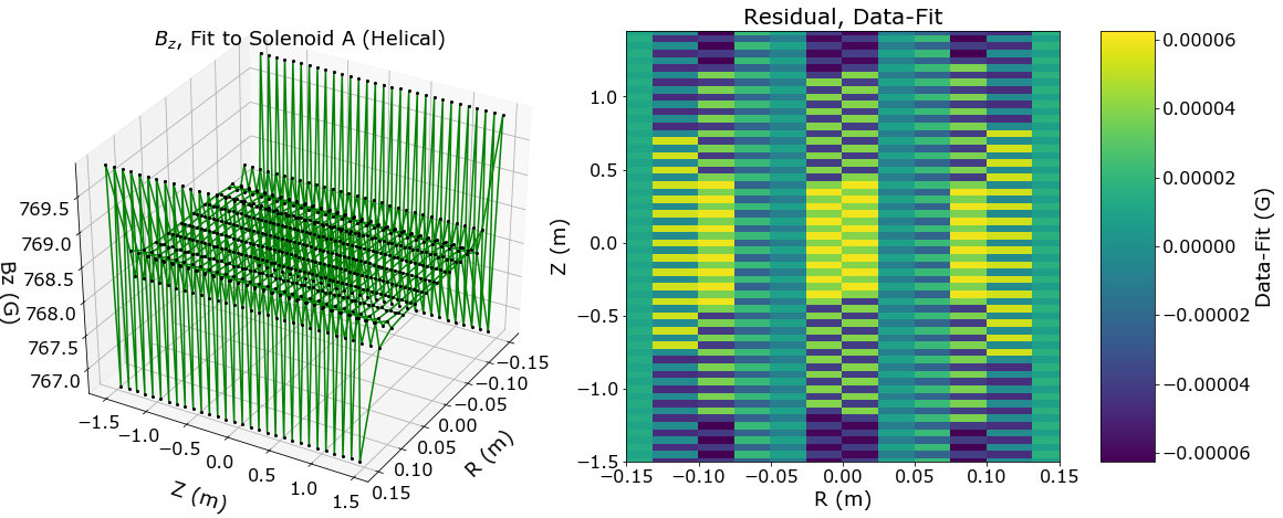 Figure 19
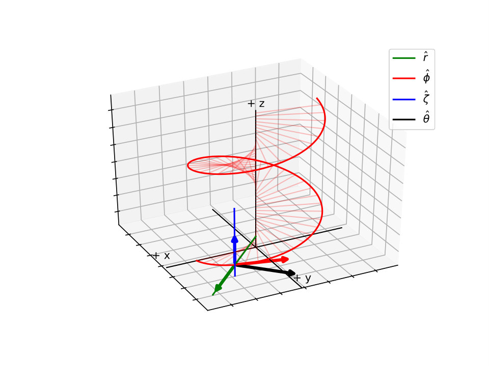 Figure 20
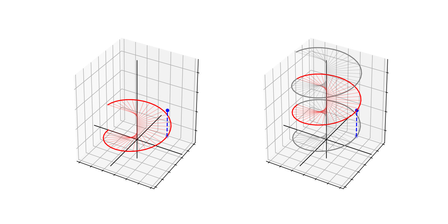 Figure 21
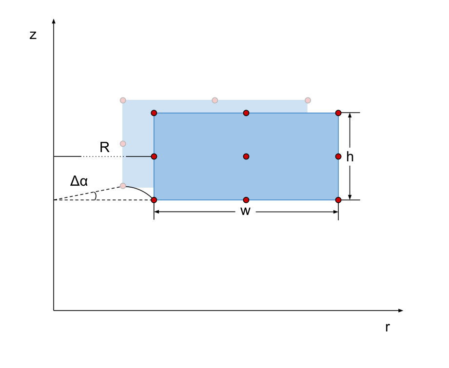 Figure 22
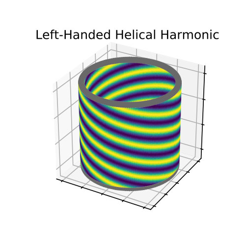 Figure 23
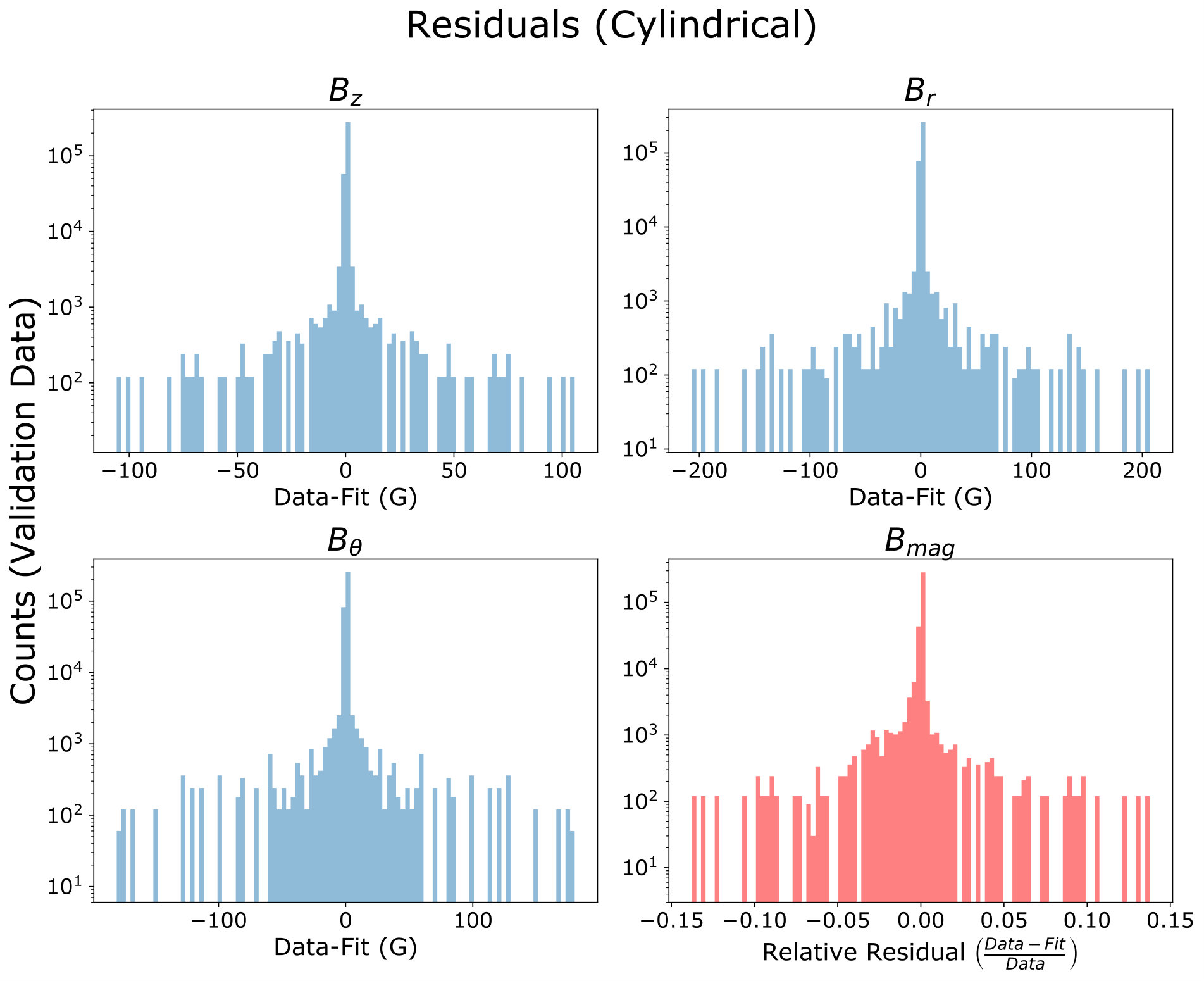 Figure 24
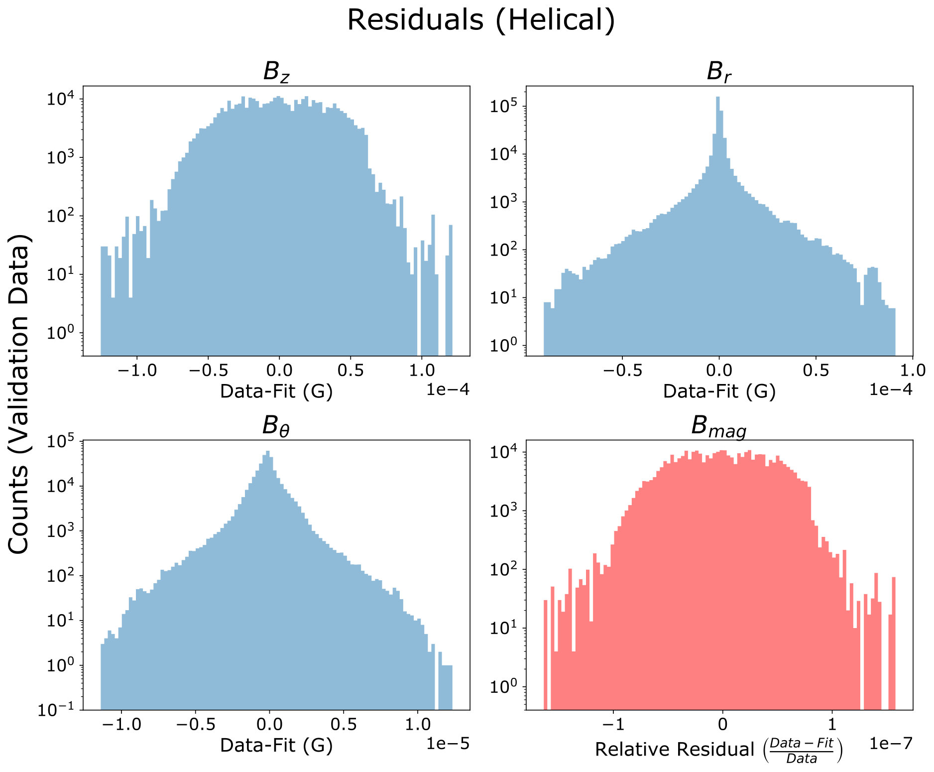 Figure 25
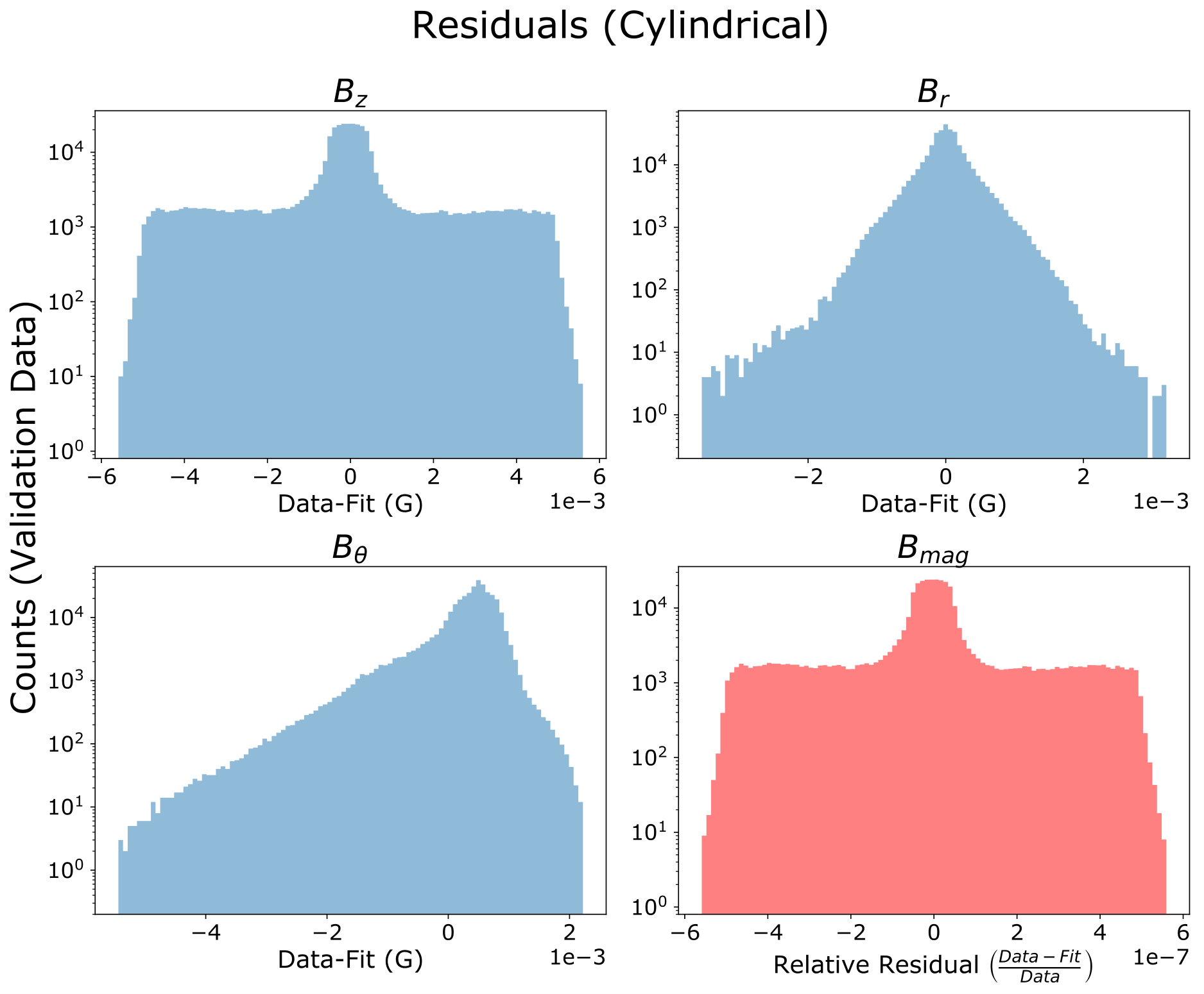 Figure 26
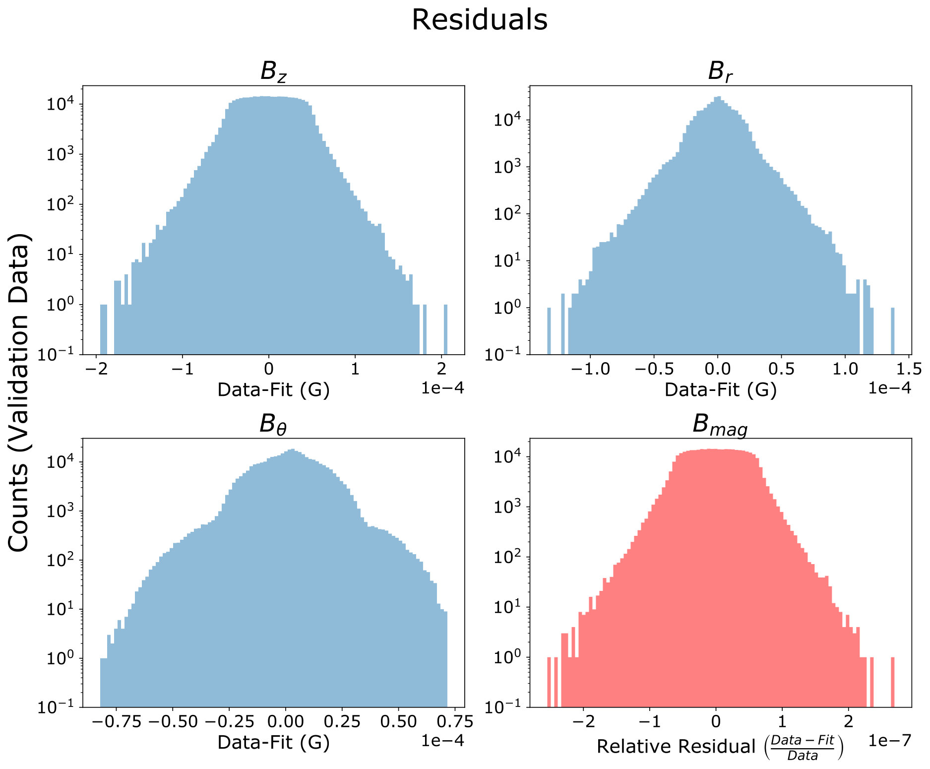 Figure 27
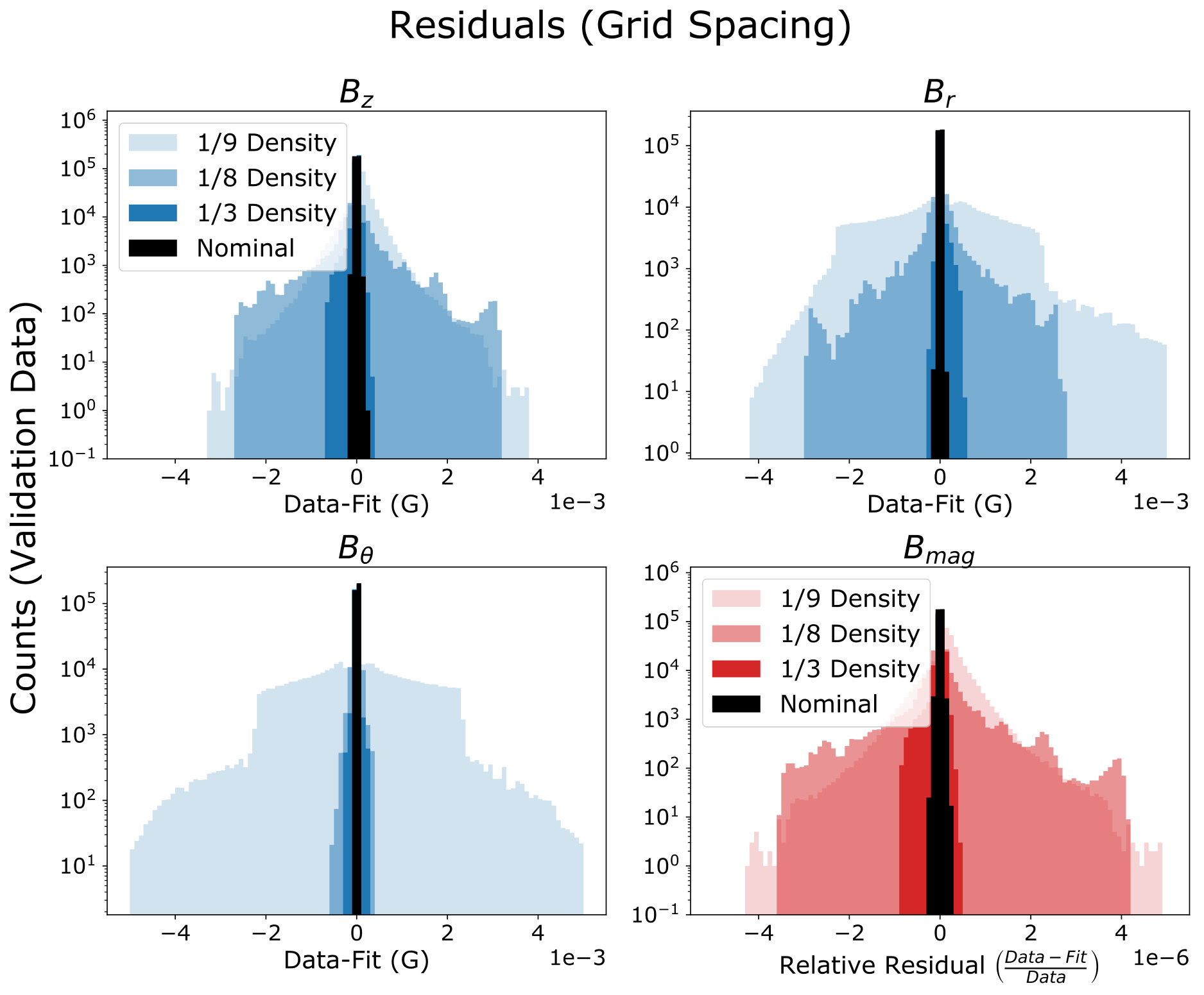 Figure 28
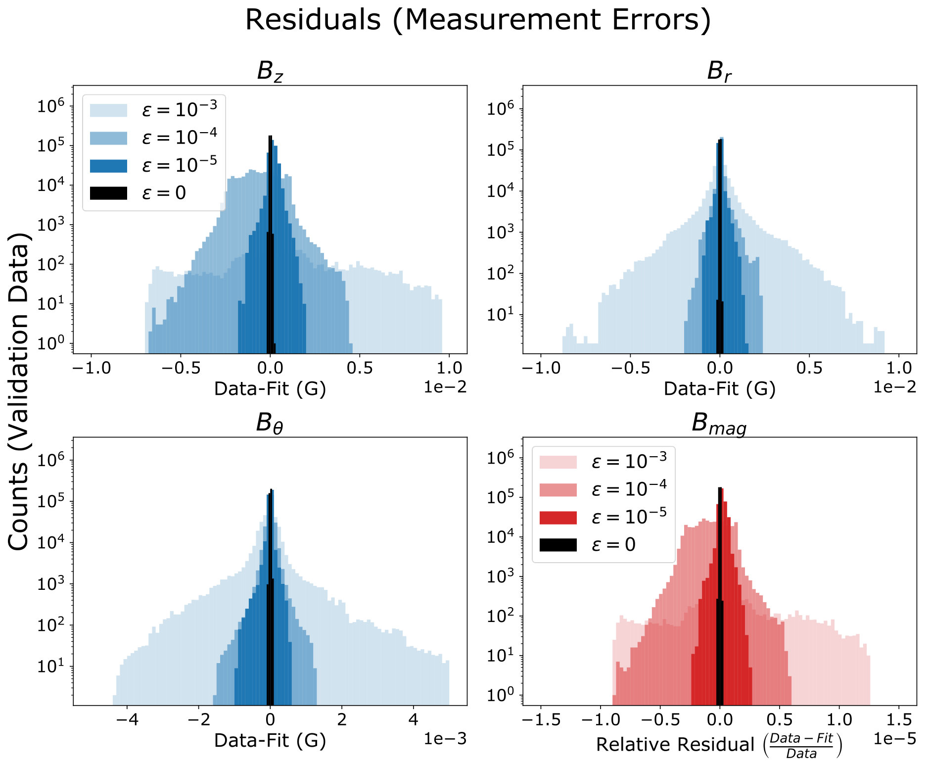 Figure 29
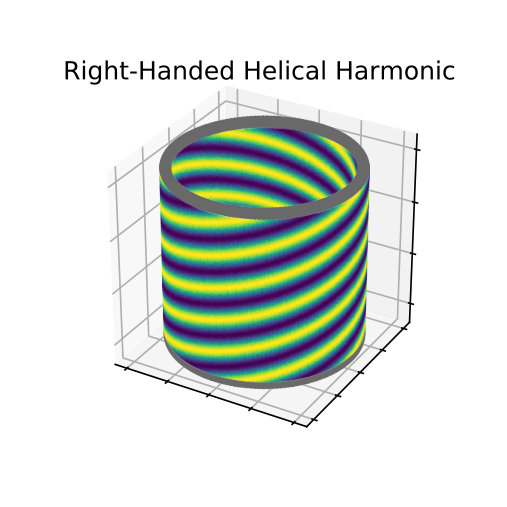 Figure 30
| Parameter | Solenoid A | Solenoid B | Solenoid C |
| Length | 92 m | 9.2 m | 9.2 m |
| Radius | 250 mm | 1000 mm | 250 mm |
| Pitch | 10 cm | 7.5 mm | 10 cm |
| Current | 6114 A | 6114 A | 6114 A |
| Average | 767 G | 1 T | 767 G |
Peer Reviews
No public reviews on file for this paper yet. If you reviewed it on a platform where reviews are public (OpenReview, ICLR, NeurIPS, ICML), you can paste yours below so the community can read it here.
Videos
No videos yet. Explain this paper in a talk, walkthrough, or lecture? Add one.
Taxonomy
TopicsGeomagnetism and Paleomagnetism Studies · Magnetic and Electromagnetic Effects · Scientific Research and Discoveries
Modeling Magnetic Fields with Helical Solutions to Laplace’s Equation
Brian Pollack
Department of Physics and Astronomy, Northwestern University, Evanston, Illinois, 60208, USA
Ryan Pellico
Department of Mathematics, Trinity College, Hartford, Connecticut, 06106, USA
Cole Kampa
Department of Physics and Astronomy, Northwestern University, Evanston, Illinois, 60208, USA
Henry Glass
Fermi National Accelerator Laboratory, Batavia, Illinois, 60510, USA
Michael Schmitt
Department of Physics and Astronomy, Northwestern University, Evanston, Illinois, 60208, USA
Abstract
The series solution to Laplace’s equation in a helical coordinate system is derived and refined using symmetry and chirality arguments. These functions and their more commonplace counterparts are used to model solenoidal magnetic fields via linear, multidimensional curve-fitting. A judicious choice of functional forms motivated by geometry, a small number of free parameters, and sparse input data can lead to highly accurate, fine-grained modeling of solenoidal magnetic fields. These models capture the helical features arising from the winding of the solenoid, with overall field accuracy at better than one part per million.
High Energy Physics; Magnetic Fields; Numerical Methods
I Introduction
The use of superconducting solenoids is commonplace in scientific research, medical, and industrial applications. The ever-increasing demand for higher resolution (e.g. medical imaging, charged particle reconstruction) requires increased accuracy and precision for the magnetic field Feher et al. (2018). The physical geometry and helical winding of a solenoid generates an axial asymmetry that may cause significant deviations of the magnetic field from that of an ideal solenoid Nouri and Plaster (2013); Gu et al. (2011), and it may be necessary to account for these deviations. The deviations will be especially pertinent for solenoidal coils that have a relatively large pitch; some large-pitch solenoids are currently employed in active particle physics experiments Wittgenstein et al. (1990); Swoboda et al. (2002). A common analysis approach used within the high energy physics community is to combine a set of sparse field measurements (e.g. provided by 2D or 3D Hall or NMR probes) with a series of functions derived from solutions to Maxwell’s equations to reconstruct the magnetic field within a given volume Amapane et al. (2005); Klyukhin et al. (2010); Aleksa et al. (2008). These methods have not attempted to use functions derived with helical symmetry, however, which may be a better choice for modeling real solenoids.
Any magnetic field must obey Maxwell’s equations. For a static field in a region free of current and magnetic materials, the magnetic field can be expressed as , where the scalar field satisfies Laplace’s equation:
[TABLE]
When treated as a boundary-value problem, Eq. 1 can sometimes be solved via a separation of variables, and in the case of solenoids, this is typically done in a cylindrical coordinate system Jackson (1999). The axial symmetry inherent to the cylindrical coordinate system is broken by the helical winding of the solenoid, however. In this case it is more appropriate to use a helical coordinate system, for which solutions to Laplace’s equation via separation of variables are known to exist Overfelt (2001). This coordinate system naturally encompasses the axial asymmetry of a helically wound solenoid, and thus is a better choice for modeling the associated magnetic field.
In this paper, we first derive the series solution to Laplace’s equation in a helical coordinate system. We then calculate magnetic fields due to solenoids with different radius, pitch, and length properties, and from those calculations produce datasets that are used as inputs for a parametric modeling of the field. Using a judicious choice of terms for the helical series, cylindrical series, and other physically valid functions for magnetic fields, we construct a model of the calculated magnetic fields using only a sparse subset of the data and a linear sum of analytical functions whose coefficients are determined through least squares fitting. We then compare the reconstructed field with a high-granularity dataset from the same calculated field in order to determine the overall precision and accuracy of the model.
This paper is structured as follows. In Section II, we introduce the mathematical formalism and solve Laplace’s equation in a helical coordinate system. In Section III, we establish the exact definitions of the functional forms used for modeling magnetic fields in the following section. In Section IV, we describe the process used to calculate helically-wound solenoids, and then model three specific examples using the functions discussed in the previous sections. For the third example, we investigate the impact of measurement error and data density on the model performance. We discuss the results and implications of these modeling efforts in Section V.
II Mathematical Formalism
Representing a scalar potential function as an infinite linear combination of orthogonal basis functions is a standard technique in potential theory, especially in service of solving boundary value problems for Laplace’s equation.
[TABLE]
The convergence of this series is understood in the sense that , as , where is the partial sum in the series representation of Evans (2010). For special geometries, various classical families of basis functions exist. For example, we will recall in what follows the various forms of the harmonic functions which separate in cylindrical coordinates, and lead to complete orthogonal bases of harmonic functions for certain function spaces Jackson (1999). For our application, it is not useful to have representations of potentials in an infinite expansion unless we can well represent the target field using only a small number of terms. We are motivated to choose the family of basis functions so that the above convergence happens as fast as possible.
Given field data for a finite set of discrete points , we propose a method to find a scalar potential function which minimizes the sum of squared residuals:
[TABLE]
We will use a series representation in terms of a family of harmonic functions which we motivate below by the geometry of a solenoid represented as a truncated helical curve. The cylindrical symmetry of a helix will cause us to work in cylindrical coordinates at first, when we recall some facts about separable cylindrical harmonics. Later we will work in a helical coordinate system introduced by Waldron Waldron (1958) and introduce a family of separable harmonic functions suited to the geometry of any particular semi-idealized solenoid. Using this functional form for the scalar potential will allow us to model features of the magnetic field that are due to the helical nature of the coil and the finite length of the solenoid.
II.1 Cylindrical Harmonics
We will briefly discuss the standard procedure of separation of variables of Laplace’s equation in cylindrical coordinates, in order to illuminate the connections to the following analogous work in the helical coordinate system.
In cylindrical coordinates , given by the standard change of variables to Cartesian coordinates , Laplace’s equation takes the following form:
[TABLE]
If we assume that separates in the cylindrical variables, , we see that the functions must satisfy the following:
[TABLE]
The quantities and are constant functions of the variables, so that , for some real constants . The function is -periodic, which forces for some integer . Consequently, must satisfy the following ordinary differential equation, which can be reduced to a Bessel equation of order using the linear change of variables , where :
[TABLE]
These relationships lead to the following forms for separable cylindrical harmonics depending on the sign of . If , then and , where and are the order Bessel functions of the first and second kind. If , then and , where and are the order modified Bessel functions of the first and second kind.
Because we are interested in potentials which do not have singularities at , we discard the Bessel functions of the second kind. Thus, for each choice of a positive integer and positive real , we have harmonic functions of the following form (note, for each term, there are three other terms corresponding to replacing and with and , respectively):
[TABLE]
This family of cylindrical harmonics is indexed by the integer and the real number . When interested in solving a boundary value problem on a cylinder , , one need only consider the countable complete orthogonal basis corresponding to choosing to be , where is an integer.
An alternative approach is to assume that and are complex exponential functions parametrized by the complex separation constants , and then determine the solution to the resulting ordinary differential equation for . In the case that the constants , and is real or purely imaginary , this approach results in the same family of harmonic functions as the standard procedure. This alternative method is used by Waldron and Overfelt Waldron (1958); Overfelt (2001) to obtain separable solutions to the wave equation and Laplace’s equation in the helical coordinate system.
II.2 Helical Coordinate Systems
An idealized infinite helix is uniquely defined by the radius , pitch111The pitch, , is defined as the advance along the axis of the helix for one complete turn. , and handedness ( or corresponding to right-handed and left-handed helices, respectively). We use the convention that a right-handed helix is one in which moving along the helix in the counter-clockwise direction (around the -axis when viewed from above) produces movement in the positive direction.
When considering an idealized helix in space, it is convenient to work in cylindrical coordinates and orient the helix so that it is contained in the cylinder given by the equation , with the -axis serving as the axis of the helix. By rotating the helix (or the coordinate system), we may assume that the helix intersects the plane on the positive axis, at the point .
With these conventions, each right-handed helix may be parametrized by the following equations, where and is a parameter representing the polar angle :
[TABLE]
Any parametrization of a helix in Cartesian coordinates will require that all three coordinates depend on the parameter , and only by orienting the helix appropriately in a cylindrical coordinate system can we parametrize the helix so that only two of the coordinates depend on that parameter. For applications in which there is helical symmetry, it is convenient to choose a coordinate system in which a helix can be parametrized using only one of the coordinates.
The following helical coordinate system was introduced by Waldron Waldron (1958), and has many similarities with a cylindrical coordinate system:
[TABLE]
We need the Jacobian of the change of variables for the above coordinate transformations, from which all of the identities concerning the coordinate directions, partial differential operators, etc. are derived:
[TABLE]
Figure 1 shows the three coordinate directions passing through a point . The helical coordinate direction is identical with it’s counterpart in cylindrical coordinates. While the coordinate direction would wind around the cylinder in a circle, the coordinate direction winds up the cylinder along a helical path. It is important to note that although for each point in space, the vectors that point in the and coordinate directions are different at each point. To be more explicit, the vector (in cylindrical coordinates) which points in the coordinate direction is the second column in Eq. 4, which has a component in the direction and a component in the direction. Since the coordinate differs from only by a translation, they are parallel: . The coordinate can be thought of as the distance in the direction between the point and the surface , illustrated by the length of the line segment Fig. 2.
With these coordinates, we may parametrize a right-handed helix with radius and pitch as follows:
[TABLE]
There is another difference between the cylindrical and helical coordinate system, relating to non-unique representations of points. In cylindrical coordinates, each point can be equivalently represented as for any integer . In helical coordinates the following more complicated identity holds for each point and each integer :
[TABLE]
This identity captures the fact that is equivalent to (i.e., changes in the coordinate which are integer multiples of are equivalent to changes in the coordinate which are the same integer multiple of the pitch ). Informally, one gets to a point pitch-lengths above by moving in only the coordinate or only in the coordinate. This identity is a consequence of the nonorthogonality of the and the coordinate directions, represented by the non-zero off-diagonal term in the Jacobian for the change of variables between cylindrical and helical; relations like this are not possible in orthogonal coordinate systems.
II.3 Helical Harmonics
In Ref. Waldron (1958), Waldron introduces the right-handed helical coordinate system as a method for analytically solving certain classic problems in electromagnetism in the case of helical symmetry. He recasts Laplace’s equation and the wave equation into helical coordinates, and then uses a modified separation of variables technique to write down explicit analytic solutions to the wave equation.
Using the same technique, Overfelt Overfelt (2001) solves Laplace’s equation in all of space and arrives at explicit forms for harmonic functions which separate in the helical coordinate system, hereafter referred to as helical harmonic functions. Here we give an overview of the technique, which parallels the method used for cylindrical coordinates.
As are functions of through the coordinate transformation equations, the chain rule
[TABLE]
together with the appropriate entries of the Jacobian (Eq. 4), allow us to recover the following relation among the differential operators in the coordinate directions:
[TABLE]
Using these relations, we can translate Laplace’s equation from cylindrical coordinates into a helical coordinate system:
[TABLE]
If we look for separable solutions to Laplace’s equation of the form where and , then satisfies the following differential equation:
[TABLE]
Equation 5 also results from the choice and . Similarly, by choosing and , or and , we find that satifies
[TABLE]
As in the cylindrical case, the ordinary differential equations for can be transformed into Bessel equations of complex order in Eq. 5 and in Eq. 6 in the variable through the linear change of variables . Thus, for arbitrary complex numbers, and , we obtain the following separable helical harmonics , in terms of Bessel functions of complex order and argument:
[TABLE]
Although the helical harmonics separate in the variables , when we add Eqs. 7 and 8, the additive property of the exponential function allows us to recover functions which couple the and variables inside the argument of trigonometric functions. Converting to cylindrical coordinates gives functions of the form which does not separate in the cylindrical variables .
In particular, choosing and in Eqs. 7 and 8, where is an integer and is a real constant, expressing the complex exponentials in terms of trigonometric functions and the Bessel functions in terms of modified Bessel functions, we arrive at the following form of real-valued helical harmonics, which we also represent in cylindrical coordinates and refer to as “left-handed” helical harmonics:
[TABLE]
The same choice of and in Eqs. 9 and 10 results in the following “right-handed” helical harmonics:
[TABLE]
Again, we have a family of harmonic functions indexed by a real parameter . For notational ease, we are free to set , and since controls the oscillations of with respect to , by setting to be integer multiples of the effective pitch, , we recover a countable family of helical harmonic functions which respect the periodicity of the solenoidal coil in .
On any cylinder , each right-handed helical harmonic function takes the following form, where is a modified Bessel function:
[TABLE]
The expression in Eq. 11 is constant along the curves in the cylinder that satisfy const. That is, it is constant along curves const, which are all the right-handed helices with pitch . If we work in a helical coordinate system with pitch , we can make by choosing and letting . It is also true that a left-handed helical harmonic function is constant along certain left-handed helices, whose pitch is determined as above. This tells us that the family introduced above contains a sequence of terms which are all constant along right-handed helices with pitch . In Fig. 3 we show cylindrical and helical harmonic functions restricted to a cylinder .
If the field is due to an idealized wire, parametrized by (Eq. 3), carrying a uniform current , then the field is given by the Biot-Savart Law:
[TABLE]
Theorem 1: A field given by the Biot-Savart Law for an idealized infinite right-handed helix with pitch leads to a field which is cylindrically symmetric along right-handed helical curves with pitch , that is for all and all , when is represented in cylindrical coordinates .
Proof.
For each real , the change of coordinates is an orientation preserving rigid motion of space under which infinite right-handed helices of pitch are invariant. is a translation of the cylindrical coordinate system along a helix with pitch , and is the composition of a rotation about the -axis by an angle and a translation in the direction with . This isometry also acts on vectors via the Jacobian , sending a vector at represented in cylindrical components, to the vector at . Since is a translation in cylindrical coordinates, the Jacobian is the identity matrix, and so the vectors and have the same cylindrical components. Now, since this rigid motion leaves the geometry of the current carrying device unchanged, since , the resulting magnetic field must be invariant under the transformation : , and the result follows. ∎
In the special case when is an integer, the translation in is an integer multiple of , so the transformation is equivalent to a pure translation in the direction with , an integer multiple of the pitch. In this case, the result of Theorem 1 is equivalent to the statement that is -periodic in . Theorem 1 implies the more general statement that in any parallel planes and , the field is identical, up to a rotation by .
Theorem 1, together with the preceding properties of the real-valued helical harmonics, leads to our choice of right-handed helical harmonic functions to model a field due to a right-handed helical solenoid, since these are precisely the harmonic functions which are constant along curves with the handedness and pitch of the solenoid.
III Functional Forms
This section details the individual functional forms used during the fitting process. Functions are expressed in either cylindrical or Cartesian coordinates, as these coordinate systems are typically used when measuring magnetic field points in solenoids, and allow for more straightforward comparisons between different forms. Functional forms are broken into three classes: “cylindrical”, “helical”, and “additional.” These classes differentiate between functions derived from series solutions to Laplace’s equation in cylindrical coordinates, series solutions to Laplace’s equation in helical coordinates, and additional functions that help with specific sources of magnetic field asymmetry.
III.1 Cylindrical Functions
Magnetic fields stemming from idealized solenoids exhibit monotonic behavior for all field components as a function of . This motivates the use of modified Bessel functions as a general solution to solenoidal magnetic fields, as modified Bessel functions exhibit monotonic behavior, while regular Bessel functions exhibit oscillatory behavior. From that equation, we can implement a fully real-valued series expression using free parameters:
[TABLE]
The coefficients , , and are determined by the fitting procedure described in Section IV. The quantity is equal to , where is some effective length scale and is used instead of in order to avoid the trivial constant term which is better handled as described in Section III.3.
Physically, the scalar potential cannot be observed or measured directly. Instead, a least-squares fit to the magnetic field components is used to determine the free parameters :
[TABLE]
where is the ordinary derivative of the modified Bessel function.
The expressions in Eq. 14 can be carried out to any number of terms in and . In practice, the truncation of these series is determined by the required modeling accuracy. In general, more asymmetric features in the -direction necessitate a larger number of terms, while more axial asymmetry necessitates a larger number of terms.
III.2 Helical Functions
As expected from the cylindrical functions, there is no direct coupling between the and variables in Eqs. 13 and 14. In order to account for axial asymmetries induced by the helical coil, one would have to expand the cylindrical series to a very large number of terms. In contrast, the helical harmonic functions link the and coordinates, and choosing the appropriate pitch parameter will lead to a large reduction in free parameters needed to obtain an accurate modeling of the magnetic field. As described in Section II.3, a right-handed helix leads to surfaces of constant potential via a right-handed series solution. The following examples are based solely on right-handed coils, so only the right-handed terms are used for the helical series expansion. From Eq. 11, the scalar field can be expressed in the following manner:
[TABLE]
where . As before, we use instead of to avoid the trivial constant term. The terms and are constants. We obtain the expressions for the magnetic field components:
[TABLE]
III.3 Additional Functions
The helical and cylindrical harmonic series expansions are constructed in the context of an infinitely long solenoid. Therefore, they are not equipped to handle constant fields, nor the edge effects from a finite solenoid; two types of behavior we expect to observe.
Constant fields can be handled simply by using a first-order Cartesian solution to Laplace’s equation. For the examples used in this paper, the solenoid axis runs along the -axis, and there is a near-constant field component. This implies that a term in the potential expansion can represent that field appropriately. In practice, by including the term we are able to reduce the total number of free parameters needed to accurately model the magnetic field. In particular, this term also replaces the zeroth order Bessel function terms (), which are the only terms capable of producing non-zero values for the magnetic field at .
The final set of terms used in the following fitting procedure are derived directly from the Biot-Savart Law (Eq. 12). An infinitesimal current located at element can be modeled using the following form:
[TABLE]
where are the free parameters associated with an effective infinitesimal current element, and . These terms are included to account for small asymmetric contributions arising from the initial and terminal endpoints of the solenoid simulations, detailed in the following section. Two of these infinitesimal current element terms are included during fitting, with the spatial free parameters () constrained to resided within of the respective endpoints.
IV Calculation and Modeling
IV.1 Calculating a Helical Solenoid
In order to determine the benefit of a helical solution to Laplace’s equation, we simulate magnetic fields due to helically-wound solenoids. Using MATLAB MATLAB (2018), we define three helical coil geometries which would be typical of high-field, large-bore solenoids used in particle physics detectors. The coils consist of flat, ribbon-like cables (Fig. 4) with a constant and homogeneous current and without any additional leads or connections. The cables have a width of 5.25 mm and a height of 2.34 mm. The magnetic fields they generate are calculated through use of the Biot-Savart law, in which a 3D, parallelized numerical integral is computed to obtain the magnetic field at a grid of points inside the coil. When performing the integral, the angular step size, , between cross-sectional planes of the cable is roughly radians. The parameters used for the different fields generated for this study are shown in Table 1.
The geometries of the three different solenoids are chosen to probe different magnetic field features. Solenoid A is long (92 m) compared to its radius (25 cm). It also has a large pitch (10 cm), which emphasizes the helical field features. These properties lead to a field that exhibits ideal helical behavior in the center region of the bore, with little impact from edge effects. Solenoid B is both shorter (9.2 m) and has a larger radius (1 m) than solenoid A. It also has a smaller pitch (7.5 mm), which reduces the helical field features to a negligible degree. This field can be modeled with cylindrical terms only. Solenoid C has geometric properties from both A and B. It has the same radius and pitch as Solenoid A, but with a length equal to Solenoid B. To model this field appropriately, we use a combination of helical and cylindrical terms.
Depictions of the field components for Solenoid C are given in Fig. 5. These magnetic fields have a relatively large, constant field in the -direction, as is characteristic of solenoids. The radial and axial components are orders of magnitude smaller than the -component (as long as one is far from the edges of the solenoid), but they are not negligible. Due to the helical nature of the solenoid, all field components exhibit wiggles in the -direction, with a wavelength given by the pitch of the solenoid.
IV.2 Fitting Magnetic Field Data
The magnetic fields can be generated using as fine a grid as required (or that computing power allows). However, a real-world solenoid cannot be surveyed on an arbitrarily fine grid. Instead, a solenoid is typically surveyed sparsely, and from that survey, the full magnetic field is reconstructed. In this section, we use the harmonic functions derived above to fit a sparse set of magnetic field values, and reconstruct a continuous field using those functions. Judicious choices of the number of parameters and length scales allow us to model a range of magnetic fields with a high degree of accuracy.
The free parameters are determined by fitting from a subset of the grid points. The remaining grid points are used for validation and visualization. The sparse subset of grid points used for fitting is selected by mimicking the process of surveying a real-world solenoid using a mechanical field mapper Feher et al. (2018). This results in a cylindrically symmetric grid with constant spacing in , the exact values of which are detailed in the following subsections.
These grid points and their associated magnetic field components, , are used as independent variables for the fit. The sum of squared residuals, (Eq. 2), is the objective function which is minimized using least-squares optimization algorithms from the Scipy and lmfit packages for the Python software language Jones et al. (01); More (1978); Branch et al. (1999); Newville et al. (2014), and linear least-squares solver in MATLAB MATLAB (2018).
In addition to either the partial derivatives of the cylindrical (Eq. 13) and/or helical (Eq. 15) series expansions, the additional terms discussed in Section III.3 are included with all fitting functions.
To determine the optimal number of terms in a given series expansion, fits are performed iteratively, increasing the number of and terms at each iteration. Once the desired accuracy is reached, no additional terms are added, even if additional terms leads to slight improvements with respect to the quality of fit. The accuracy requirements for the three solenoid examples are discussed in more detail in the following sections.
Additional studies are performed on Solenoid C, in order to investigate the impact of measurement error and grid density on the fit performance. Gaussian noise is introduced to the sparse field component values to emulate measurement error. The density of the sparse grid is varied, reducing the total number of data available during fitting.
IV.2.1 Solenoid A
Solenoid A (Table 1) is intended to bring out the helical features that arise from the winding of the solenoid, while minimizing edge effects. The solenoid is very long with respect to its radius, has a relatively large pitch, and region of interest is restricted to the middle of the solenoid, far from the edges. This region is fit with two different series expansions: the cylindrical expansion (Eq. 14) and the helical expansion (Eq. 16) in order to ascertain which expansion leads to greater accuracy and fewer terms. The two expansions are compared using the objective function (Eq. 2), the per-component residuals, and the overall accuracy using the validation data set.
The sparse set of data selected to fit for Solenoid A consists of 6 radial positions, chosen such that , 16 equally-spaced angles from 0 to 2, and 60 equally-spaced positions . The total number of data points is 5760, and each point contains three magnetic field vector components, . The validation dataset is generated from a selection of 24 equally spaced radial positions from , 126 equally spaced angles, and 120 equally spaced Z positions, leading to a total of 362,880 data points. These points were chosen to probe a region far from the edges of the solenoid to minimize edge effects, and far enough from the solenoid coil to avoid discontinuities while still capturing the helical wiggles. The pitch, , chosen for the helical series is 10 cm, identical to the pitch used to generate the solenoid. The length scale, , used for the cylindrical series is 5 cm. This length scale was chosen such that for Eqs. 14 and 16, which determines the wavelength of the wiggles in the -direction.
An example of the fits, with associated residuals, are shown in Figs. 6 and 7. The 3D plots on the left-hand side show the values of the field components with both the calculated data (black points) and the fit function (green mesh) for a single 2D plane of measurements. Note that the parametric fit was determined using a full 3D selection of points, not just the 2D plane displayed. In all three components, the wiggles due to the helical coil are significant, especially at the outer radius of the fit. The size of the wiggles from peak to trough are roughly 3-4 G for the component and roughly 0.2-0.3 G for the and components. The residuals, expressed as Data-Fit in units of Gauss, are shown on the right-hand sides of the plots. The vertical striping (especially prominent in the upper right plot of Fig. 6, for example) corresponds to each of the radial positions used in the sparse data set, as the residuals are only evaluated at each of the fitted points for these plots. The horizontal striping corresponds to the variation in the residuals as a function of the step size. While the left-hand plots for the helical and cylindrical fits may look equivalent, the upper and lower bounds on the residuals for the helical fit are between two to three orders of magnitude smaller than the those of the cylindrical fit. The fit to helical harmonic functions is much more accurate than the fit to cylindrical functions.
The quality of the fits as a function of the total numbers of terms and is shown in Fig. 8. For both the cylindrical and helical expansions, the terms multiply the coordinate inputs and the terms multiply the coordinate inputs. The helical series requires only a few terms in the expansion before it reaches a point where additional terms do not greatly improve the quality of fit. In contrast, the cylindrical series continually improves as the number of terms increases, until determining the optimal free parameter values becomes too computationally taxing. Even at roughly 10 times the number of free parameters, the cylindrical expansion does not reach the level of fit quality found using the helical expansion.
The residuals derived from the validation dataset are shown in Fig. 9 for both the helical and cylindrical series. Note that the range of the horizontal axis for the cylindrical and helical plots are vastly different; the range for the helical plot is about six orders of magnitude smaller than the cylindrical. At its worst, the range of the residuals for the helical series are at least four orders of magnitude better than the residuals for the cylindrical series, and with roughly 10 times fewer free parameters. As expected, the helical series is the superior choice for this example, and the relative residuals on the overall magnitude of the field are typically much better than 0.1 parts per million.
The set of terms chosen to construct the validation plots (Fig. 9) was and . Additional terms only added a one to two percent improvement to the statistic, as can be seen from Fig. 8. In Section II.3, terms in which (or , due to the redefinition in Section III.2) are shown to lead to solutions for constant helical surfaces for a given pitch for a right handed helix. The results in Fig. 8 confirm that prediction; there is a large improvement in the residuals for both the terms and the terms. The cylindrical series used for validation used and , as additional terms produced no improvement to the metric or the residual validation plots.
IV.2.2 Solenoid B
Solenoid B differs from Solenoid A in three distinct ways: it has a larger radius (1 m), a smaller pitch (7.5 mm), and a shorter length (9.2 m) than Solenoid A. The field has a roughly 1 T component, and and components that are 3-5 orders of magnitude smaller. These properties lead to a magnetic field which does not exhibit helically-induced wiggles in the field except very close to the coil. Additionally, the large radius and small pitch lead to a large radius-to-pitch ratio, which presents challenges to the helical harmonic series. A very large () radius-to-pitch ratio is difficult to use because it is the argument of the modified Bessel functions used in the helical series expansion. This large argument causes the Bessel functions to grow until they are computationally unwieldy (). The shorter length of the solenoid impacts the uniformity of the field components as a function of , such that they vary smoothly over the length of the solenoid. In order to address all these features, the cylindrical series expansion is used instead of the helical series, where the input length scale, , is the total length of the solenoid. The results of this example are used to motivate the parameterization of the fit to Solenoid C, which is a hybrid of Solenoids A and B.
The sparse data set used for fitting consists of the same and selection used for Solenoid A, along with 6 radial positions between 15 and 90 cm, in 15 cm increments. Examples of the fits to Solenoid B are shown in Fig. 10. As for the to Solenoid A fits, the horizontal and vertical striping in the residual plots is a consequence of the discrete nature of fit data. The oscillations in the residuals, especially prominent in the residuals, are due to the shorter wavelength terms used in the parameterization. If more terms were added to the parameterization, the magnitude of these oscillations would be reduced. To determine the number of terms to include in the series expansion, the fits were conducted iteratively, increasing the number of terms with each iteration. The results of these fit iterations are shown in Fig. 11. Based on these results, the series is expanded to and , as additional terms only lead to diminishing (1-2%) improvements to the residuals.
The validation set used to determine the per component residuals for this model is identical in and with respect to Solenoid A, and used 24 equally spaced radial steps between 3.75 cm and 90 cm. The residuals based on the validation data are shown in Fig. 12. The residuals are never larger than G, and are typically much smaller. Overall, the residuals are smaller than 1 part per million. The skewness of the residual plot for , which affects about 1% of the validation dataset, is driven by an unavoidable asymmetry due to first and last turns of the solenoid, which deviate from an ideal cylinder. This can be seen in the residual plot of Fig. 10, specifically the darker blue regions in the upper and lower left corners corresponding to the residuals at large radius and m.
IV.2.3 Solenoid C
Solenoid C is identical to Solenoid A in all respects except for length; it is the same length as Solenoid B, (10 times shorter than Solenoid A), which enhances the -dependent, -independent features of the magnetic field due to the finite nature of the solenoid. As can be seen in Fig. 5, Solenoid C has both the large scale, smooth variation of Solenoid B in addition to the high frequency wiggles of Solenoid A. To model this simulation appropriately, a combination of terms is used from both the helical and cylindrical series expansions.
The sparse set of data selected to fit for Solenoid C, as well as the set of validation data, are identical to the sets used for Solenoid A. Instead of performing a scan over a very large potential space of terms, the number of terms for Solenoid A ( and for helical) is combined with the number of terms for Solenoid B ( and for cylindrical), and all parameters are free. Examples of the fit to Solenoid C are shown in Fig. 13. The residual plots indicate that the fields are modeled very well, with only small ( G) variations between fit and data. The residuals based on the validation dataset, shown in Fig. 14, are on the order of G or less for all field components, and the residuals for the total field magnitude are better than one part per million, which indicates that this combination of terms works well for modeling all major features of this magnetic field.
Two further studies were performed on Solenoid C. The first study investigated the effect of varying the density of the sparse data used for fitting, and the second study explores the effect of measurement error on the fit data.
In the first study, the original sparse data for fitting Solenoid C is a cylindrical lattice whose coordinates are one of 6 radial positions, 16 angular positions, and 60 positions. The total number of data points is 5760. We can specify subgrids by selecting subsets of each of the radial, angular, and positions.
Fig. 15 shows the residuals for fits using subgrids with 1/3, 1/8, and 1/9 of the density of the original fitting grid. The 1/3 and 1/9 density subgrids are formed by selecting every and every point among the positions, respectively. The 1/8 density subgrid is formed by taking every other point in each of the radial, angular, and positions. It is clear that the error increases as the density decreases, but even the largest relative error in magnitude is still on the order for the sparsest grid. We also note that the original grid is already a very coarse subgrid of the fine grid used for validation. The details of these grids are shown in Section IV.2.3.
[TABLE]
The second study examines the response of our method to measurement error on the fit data. For modern solenoid mapping, NMR and Hall probes are required to have measurement accuracy on the order of hall_probe. In order to simulate this type of measurement error, Gaussian noise is added independently to each field component in the data before fitting. The Gaussian mean is 0 and the standard deviation in each component is chosen to simulate a relative error of . The residuals are calculated by comparing the fit values to the true field values ().
Fig. 16 shows histograms of the residuals for fits with . The histogram for corresponds to the nominal fit as seen in Fig. 14. The error leads to a relative residual of better than for the majority of data points, and even the most pessimistic error simulations are typically less than . This implies that our method is robust with respect to expected measurement errors for magnetic field surveys.
V Summary and Conclusions
Starting from first principles, we have introduced general solutions to Laplace’s equation in a helical coordinate system for the purposes of modeling realistic solenoidal magnetic fields. Using sparse sets of data generated for different solenoidal geometries, we modeled the magnetic field using expansions of helical and cylindrical harmonic functions and validated the model with a high-granularity magnetic field calculation. Using a small number of free parameters, we were able to obtain accurate magnetic field models, and capture asymmetric behavior caused by the helical coil. The residuals are better than one part per million, and typically better than 0.1 parts per million.
The helical series expansion is good at capturing the wiggles that arise from the helical winding of a solenoid. Depending on the pitch and radius of the solenoid, these oscillations can become significant compared to the average field strength, and ignoring these contributions would lead to an incorrect model of the magnetic field. The cylindrical series are useful for modeling the low frequency components of a finite-length solenoid. Using an effective length equal to the solenoid length, the cylindrical series models the -dependent, axially symmetric features of the magnetic field. For solenoids of both finite length and with helical features, a combination of helical and cylindrical series solutions provides the most accurate model. While not exhaustive, we examined the impact of realistic measurement errors on our model. Even with pessimistic error assumptions, our model still performs well, with residuals better than 10 parts per million, and typically better than 1 part per million. Further studies of magnetic field perturbation due to machining tolerances, external magnetic field sources (e.g. due to additional circuitry), and other sources of error are left for future investigation.
While this method was shown to be useful for representing a magnetic field, it can also be used to calculate a magnetic field. The calculated fields used in this paper were generated using a common numerical integration of the Biot-Savart law. This process, even when parallelized across GPUs, is computationally taxing, and its resource usage scales both as a function of the size of the solenoid and the number of grid points in which one would like to evaluate the field. Conversely, starting with a closed-form solution of a complex magnetic field scales to the number of grid points, and the evaluation of each grid point requires executing only a handful of mathematical terms instead of a series of numeric integrals. While the method for determining the coefficients of this series without the use of fitting is not explored in this paper, it should be possible for an appropriately specified field calculation to do so.
Acknowledgements.
The authors would like to thank Matt Bonakdarpour for helpful discussions. We gratefully acknowledge the support provided by the Department of Energy under award number DE-SC0015910. This document was prepared by members of the Mu2e Collaboration using the resources of the Fermi National Accelerator Laboratory (Fermilab), a U.S. Department of Energy, Office of Science, HEP User Facility. Fermilab is managed by Fermi Research Alliance, LLC (FRA), acting under Contract No. DE-AC02-07CH11359. We thank the reviewers for providing helpful comments on earlier drafts of the manuscript.
The reference list from the paper itself. Each links out to its DOI / PubMed record.
- 1Feher et al. (2018) S. Feher, P. De Lurgio, L. Elementi, H. W. Friedsam, J. J. Grudzinski, M. J. Lamm, J. M. Nogiec, C. Orozco, B. Pollack, M. H. Schmitt, T. Strauss, R. L. Talaga, R. G. Wagner, J. L. White, and H. Zhao, IEEE Transactions on Applied Superconductivity 28 , 1 (2018) . · doi ↗
- 2Nouri and Plaster (2013) N. Nouri and B. Plaster, Nuclear Instruments and Methods in Physics Research Section A: Accelerators, Spectrometers, Detectors and Associated Equipment 723 , 30 (2013) . · doi ↗
- 3Gu et al. (2011) X. Gu, M. Okamura, A. Pikin, W. Fischer, and Y. Luo, Nuclear Instruments and Methods in Physics Research Section A: Accelerators, Spectrometers, Detectors and Associated Equipment 637 , 190 (2011) . · doi ↗
- 4Wittgenstein et al. (1990) F. Wittgenstein, A. Herve, M. Feldmann, D. Luckey, and I. Vetlitsky, “Construction of the l 3 magnet,” in 11th International Conference on Magnet Technology (MT-11): Volume 1 , edited by T. Sekiguchi and S. Shimamoto (Springer Netherlands, Dordrecht, 1990) pp. 130–135. · doi ↗
- 5Swoboda et al. (2002) D. Swoboda, L. Leistam, L. Pigni, D. E. Cacaut, E. Kochournikov, and A. S. Vodopyanov, IEEE Trans. Appl. Supercond. 12 , 432 (2002) .
- 6Amapane et al. (2005) N. Amapane, V. Andreev, V. Drollinger, V. Karimaki, V. Klyukhin, and T. Todorov, (2005) .
- 7Klyukhin et al. (2010) V. I. Klyukhin, N. Amapane, V. Andreev, A. Ball, B. Cure, A. Herve, A. Gaddi, H. Gerwig, V. Karimaki, R. Loveless, M. Mulders, S. Popescu, L. I. Sarycheva, and T. Virdee, IEEE Transactions on Applied Superconductivity 20 , 152 (2010) . · doi ↗
- 8Aleksa et al. (2008) M. Aleksa, F. Bergsma, P. A. Giudici, A. Kehrli, M. Losasso, X. Pons, H. Sandaker, P. S. Miyagawa, S. W. Snow, J. C. Hart, and L. Chevalier, Journal of Instrumentation 3 , P 04003 (2008) .