Monotone Least Squares and Isotonic Quantiles
Alexandre M\"osching, Lutz Duembgen

TL;DR
This paper develops nonparametric methods for estimating isotonic distribution and quantile functions in bivariate data, establishing their convergence rates and relationships under stochastic order assumptions.
Contribution
It introduces two related monotone least squares estimators for distribution and quantile functions, analyzing their properties and convergence rates.
Findings
Establishes convergence rates for the estimators.
Shows the close relationship between distribution and quantile estimation methods.
Demonstrates the flexibility of the distribution-based approach over quantile-based methods.
Abstract
We consider bivariate observations such that, conditional on the , the are independent random variables with distribution functions , where is an unknown family of distribution functions. Under the sole assumption that is isotonic with respect to stochastic order, one can estimate in two ways: (i) For any fixed one estimates the antitonic function via nonparametric monotone least squares, replacing the responses with the indicators . (ii) For any fixed one estimates the isotonic quantile function via a nonparametric version of regression quantiles. We show that these two approaches are closely related, with (i) being more flexible than (ii). Then, under mild regularity conditions, we establish rates of…
Click any figure to enlarge with its caption.
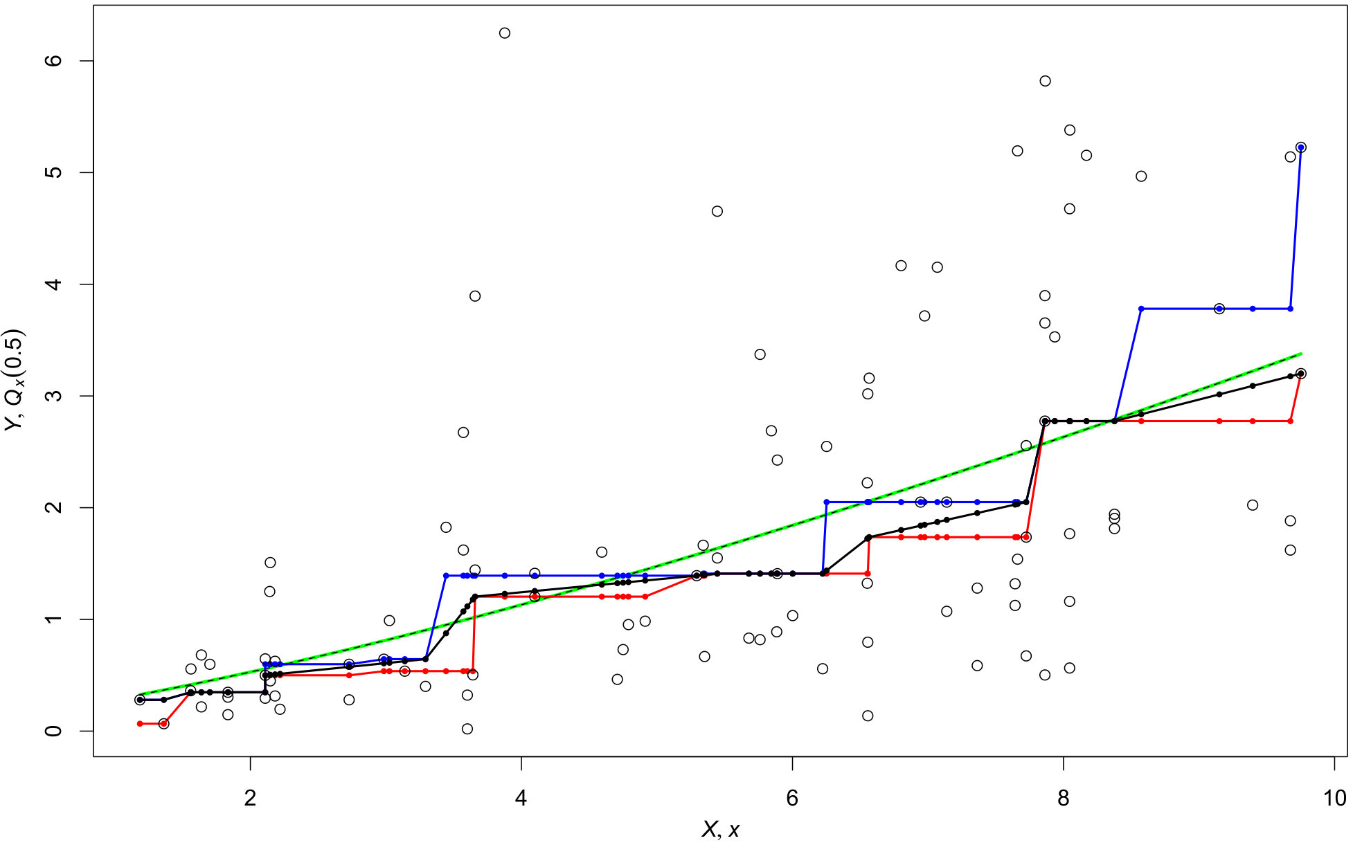 Figure 1
Peer Reviews
No public reviews on file for this paper yet. If you reviewed it on a platform where reviews are public (OpenReview, ICLR, NeurIPS, ICML), you can paste yours below so the community can read it here.
Videos
No videos yet. Explain this paper in a talk, walkthrough, or lecture? Add one.
Monotone Least Squares and Isotonic Quantiles
Alexandre Mösching, Lutz Dümbgen
University of Bern
Abstract
We consider bivariate observations such that, conditional on the , the are independent random variables with distribution functions , where is an unknown family of distribution functions. Under the sole assumption that is isotonic with respect to stochastic order, one can estimate in two ways:
(i) For any fixed one estimates the antitonic function via nonparametric monotone least squares, replacing the responses with the indicators .
(ii) For any fixed one estimates the isotonic quantile function via a nonparametric version of regression quantiles.
We show that these two approaches are closely related, with (i) being more flexible than (ii). Then, under mild regularity conditions, we establish rates of convergence for the resulting estimators and , uniformly over and in certain rectangles as well as uniformly in or for a fixed .
Keywords:
Regression quantiles, stochastic order, uniform consistency.
AMS 2000 subject classifications:
62G08, 62G20, 62G30.
1 Introduction
Suppose we observe pairs
[TABLE]
with random or fixed covariate values in a set such that, conditional on , the response values are independent with
[TABLE]
for and . Here is an unknown family of distribution functions on . Note that some values could be identical, so the corresponding random variables have the same conditional distribution, given .
Our goal is to estimate the whole family under the sole assumption that is isotonic (non-decreasing) with respect to stochastic order. This can be expressed in three equivalent ways:
(SO.1) For arbitrary fixed , is antitonic (non-increasing) in .
(SO.2) For any fixed , the minimal -quantile is isotonic in .
(SO.3) For any fixed , the maximal -quantile is isotonic in .
In what follows, we denote with any -quantile of and assume that it is isotonic in .
Such a constraint appears natural in several settings. For instance, an employee’s income tends to increase with his or her age . Other examples in which such a stochastic order is plausible are: The expenditures of a household for certain goods in relation to its monthly income ; the body height or weight of a child in relation to its age . Stochastic ordering constraints also have applications in forecasting. For example, and could be the predicted and actual cumulative precipitation amounts on different days, respectively, with the predictions being obtained from a numerical weather prediction model, see Henzi (2018).
With condition (SO.1) in mind, one could think about estimating the antitonic function by means of monotone least squares regression, replacing the response values with the indicator variables . Precisely, we would set with an antitonic function such that
[TABLE]
is minimal. The solution is unique on the set , and on one could extrapolate it in some reasonable way. In the special case of being finite this approach has been proposed and analyzed by El Barmi and Mukerjee (2005).
Conditions (SO.2-3) suggest to imitate the regression quantiles of Koenker and Bassett (1978). That means, we estimate the conditional -quantiles by with an isotonic function minimizing the empirical risk
[TABLE]
where denotes the loss function
[TABLE]
This estimator has been considered, for instance, by Poiraud-Casanova and Thomas-Agnan (2000) who showed that it coincides with an estimator of Casady and Cryer (1976) which is given by a certain minimax formula involving sample -quantiles. The characterization of isotonic estimators in terms of minimax formulae has also been derived by Robertson and Wright (1980) in a rather general framework including arbitrary partial orders on and general loss functions R_{i}(\makebox[4.30554pt]{{\cdot}}) in place of \rho_{\beta}(Y_{i}-\makebox[4.30554pt]{{\cdot}}), see also Section 4.1.
The goals of the present paper are to clarify the connection between these two estimation paradigms and to provide new consistency results in a suitable asymptotic framework.
In Section 2, we give a detailed description of the estimator based on monotone least squares and estimators based on monotone regression quantiles. Then we show that the estimators are essentially quantiles of the estimators , but the latter allow for smoother estimated quantile curves.
In Section 3, we analyze the estimators in a suitable asymptotic framework with a triangular scheme of observations and being a real interval. It turns out that under certain regularity conditions on the design points and the true distribution functions , one can prove rates of convergence for quantities such as
[TABLE]
with intervals , and . These results generalize and improve the findings of Casady and Cryer (1976), see also Mukerjee (1993) who analyzed a slightly different estimator. In addition we investigate
[TABLE]
for a fixed interior point of . These results complement the analysis of a single quantile curve by Wright (1984).
Proofs and technical details are deferred to Section 4. We also provide some general results about isotonic regression which are of independent interest.
2 Estimation of the conditional distributions
Throughout this section, we view the observations , , as fixed and focus mainly on computational aspects. Let be the different elements of the set of observed values , that means, . For , we set
[TABLE]
Then
[TABLE]
and the unconstrained maximum likelihood estimator of is given by
[TABLE]
2.1 Estimation of via monotone least squares
The estimator in (1) is rather poor by itself, unless the corresponding subsample size is large. But in connection with our stochastic order constraint, it becomes a useful tool. Note first that, for any function ,
[TABLE]
and the stochastic order assumption implies that the vector belongs to the cone
[TABLE]
Hence one can estimate by the unique least squares estimator
[TABLE]
It is well-known that may also be represented by the following minimax and maximin formulae, see Robertson et al. (1988): For ,
[TABLE]
where
[TABLE]
and stand for indices in such that . These formulae are useful for theoretical considerations. In particular, since the pointwise maximum or minimum of finitely many distribution functions is a distribution function, too, we may conclude that for ,
[TABLE]
The computation of is easily accomplished via the pool-adjacent-violators algorithm (PAVA), see Robertson et al. (1988). Note also that it suffices to compute for at most different values of . Precisely, if are the elements of , then for , for , and for and . Consequently, since the PAVA is known to have linear complexity, the computation of all estimators , , requires steps.
Finally, we extrapolate to an antitonic function on . We set for and for . For , , one could define by linear interpolation, but other antitonic interpolations are possible without affecting our asymptotic results.
2.2 Plug-in estimation of
Once we have estimated by as in Section 2.1, we can easily determine corresponding quantile functions. For any fixed and , , we could determine the minimal and maximal -quantiles,
[TABLE]
Both vectors and are isotonic, and any choice of an isotonic function such that , , is a plausible estimator of a -quantile curve.
2.3 Estimation of via monotone regression quantiles
Similarly as in Section 2.1, we focus on the vector . Writing
[TABLE]
one can estimate by some vector in the set
[TABLE]
where and
[TABLE]
Note that the function T_{\beta}(\makebox[4.30554pt]{{\cdot}}) is convex but not strictly convex on . Hence it need not have a unique minimizer. The next result provides more precise information in terms of the minimal and maximal sample -quantiles
[TABLE]
Lemma 2.1.
The set is a compact and convex subset of .
Two particular elements of are the vectors and with components
[TABLE]
Any vector satisfies componentwise.
On the other hand, suppose that satisfies and that is a subset of . Then .
Finally, for any , the set contains no data point .
Remark 2.2.
At first glance, one might suspect that any isotonic vector satisfying minimizes . But this conjecture is wrong. As a counterexample, consider the case of observations with but . Here , and , and
[TABLE]
Hence
[TABLE]
because , and
[TABLE]
But
[TABLE]
because for with ,
[TABLE]
with equality if, and only if, .
2.4 Connection between the two estimation paradigms
Restricting the plug-in quantile estimators of Section 2.2 to the set of observed -values leads to the set
[TABLE]
This set is closely related to the set :
Lemma 2.3.
The vectors and in Lemma 2.1 are given by
[TABLE]
In particular, .
Example 2.4.
The simple example in Remark 2.2 shows that in general. Let us illustrate this point with a more interesting numerical example. Figure 1 shows a simulated sample of size . In addition, it shows the minimal and maximal median curves obtained by linear interpolation of the points and , respectively, as well as a piecewise linear median curve minimizing among all isotonic functions such that , . Although is a natural candidate and smoother in than or , the corresponding values of T_{0,5}(\makebox[4.30554pt]{{\cdot}}) are (rounded to three digits)
[TABLE]
The true medians are depicted as well.
3 Asymptotic considerations
We provide some asymptotic properties of the estimators just introduced in case of a real interval and a triangular scheme of observations: For each sample size , consider observations with such that conditional on , the random variables are independent with
[TABLE]
for and . The resulting constrained estimators of and are denoted by and , respectively. In what follows, we derive asymptotic properties of these estimators under moderate assumptions, where asymptotic statements refer to .
El Barmi and Mukerjee (2005) derived asymptotic properties in case of a fixed finite set , which is easier to handle than the present setting.
3.1 Uniform consistency in both arguments
First of all, we assume that the distribution functions are Hölder-continuous in , at least on some subinterval of :
(A.1)
For given intervals and , there exist constants and such that
[TABLE]
Secondly, we assume that the design points are ‘asymptotically dense’ within this interval . To state this precisely, we need some notation. We write
[TABLE]
and \lambda(\makebox[4.30554pt]{{\cdot}}) stands for Lebesgue measure. Moreover, the absolute frequency of the design points is denoted by w_{n}(\makebox[4.30554pt]{{\cdot}}), that means,
[TABLE]
(A.2)
For given constants , let be the event that for arbitrary intervals ,
[TABLE]
Then,
[TABLE]
Remark 3.1** **(Fixed design points).
Suppose that with real numbers , and let for . Then Assumption (A.2) is satisfied for any fixed and .
Remark 3.2** **(Random design points).
Suppose that are independent random variables with density on such that on . With standard results from empirical processes on the real line, including exponential inequalities for beta distributions, we can show that for any choice of , and ,
[TABLE]
with asymptotic probability one as . Hence Assumption (A.2) is satisfied.
Under the two assumptions above, the estimator satisfies a uniform consistency property.
Theorem 3.3.
Suppose that Assumptions (A.1–2) are satisfied. Then there exists a such that
[TABLE]
where .
Concerning estimated quantiles, we combine Assumptions (A.1–2) with a growth condition on the conditional distribution functions :
(A.3)
For some numbers and ,
[TABLE]
for arbitrary and such that and .
For instance, if each , , has a density such that
[TABLE]
then (A.3) is satisfied with the latter parameter .
Theorem 3.4.
Suppose that Assumptions (A.1–3) are satisfied with in (A.1). Then, for any plug-in estimator of ,
[TABLE]
where and are defined as in Theorem 3.3, and denotes the interval .
3.2 Uniform consistency at a single point
In addition to the previous uniform convergence results, one may verify uniform consistency of and for a fixed interior point of . These results require similar but weaker assumptions.
(A’.1)
For a neighbourhood of and an interval , there exist constants and such that
[TABLE]
(A’.2)
For given constants , let be the event that
[TABLE]
Then,
[TABLE]
Under these two assumptions, the following consistency property holds.
Theorem 3.5.
Suppose that Assumptions (A’.1–2) are satisfied. Then
[TABLE]
(A’.3)
For some numbers and ,
[TABLE]
for arbitrary such that and .
Theorem 3.6.
Suppose that Assumptions (A.1–3) are satisfied with in (A.1). Then, for any plug-in estimator of ,
[TABLE]
where and .
4 Proofs and technical details
4.1 Monotone regression
In this section we review isotonic regression on a totally ordered set in a rather general setting, summarizing and extending results of numerous authors. Our main goal is a thorough understanding of isotonic regression in situations with potentially non-unique solutions. For extensions to partially ordered sets we refer to Mühlemann et al. (2019).
The starting point are loss functions with the following property: For arbitrary indices , the function
[TABLE]
is minimal on a compact interval , strictly antitonic on and strictly isotonic on .
This property is satisfied if all functions are convex with as . It implies a refined version of the so-called Cauchy-mean-value property.
Proposition 4.1.
Let be partitioned into index intervals . Then
[TABLE]
Proof.
The smallest minimizer of is the largest real number such that is strictly antitonic on and the smallest real number such that is isotonic on . Since , this function is strictly antitonic on \bigcap_{1\leq i\leq k}(-\infty,L_{a_{i}b_{i}}]=\bigl{(}-\infty,\min_{1\leq i\leq k}L_{a_{i}b_{i}}\bigr{]} and isotonic on \bigcap_{1\leq i\leq k}[L_{a_{i}b_{i}},\infty)=\bigl{[}\max_{1\leq i\leq k}L_{a_{i}b_{i}},\infty\bigr{)}. This yields the desired inequalities for . The largest minimizer can be handled analogously. ∎
Now we consider the function ,
[TABLE]
and the set
[TABLE]
The elements of can be characterized completely in terms of the minimizers of the functions . Throughout the sequel, we set and for a vector . Moreover, the componentwise minimum and maximum of vectors are denoted by and , respectively.
Proposition 4.2.
For a vector , the following two properties are equivalent:
(i) .
(ii) For arbitrary indices ,
[TABLE]
This characterization is a generalization of Theorem 8.1 of Dümbgen and Kovac (2009).
Proof of Proposition 4.2.
We first show that property (i) is equivalent to a seemingly weaker version of (ii):
(ii’) For arbitrary indices ,
[TABLE]
Suppose that property (ii’) is violated. Specifically, for some indices , let but . Since is strictly isotonic on ,
[TABLE]
defines a vector such that . Analogously, if but , one can find a vector such that . This shows that property (i) implies property (ii’).
Suppose that property (ii’) is satisfied, and let be an arbitrary vector in . If for some index , let be the smallest such index, and let be the largest index with . Thus and . Now we repeat the following step until : We choose the smallest index such that . Property (ii’) implies that , so is isotonic on . Consequently, if we replace with the smaller number , the value does not increase. These considerations show that replacing with yields a new vector with the same or a smaller value of . Repeating this construction finitely often shows that replacing with does not increase . Analogously one can show that replacing with does not increase . Combining both steps shows that the original vector satisfies the inequality . Hence belongs to .
It remains to show equivalence of properties (ii) and (ii’). The latter is obviously a consequence of the former one. Hence it suffices to show that a violation of property (ii) implies a violation of (ii’). Consider indices such that but . In case of , this is a violation of property (ii). In case of we partition into maximal index intervals on which is constant. Then , whereas Proposition 4.1 yields the inequality . Hence for some index , but , a violation of (ii). The situation that but can be handled analogously. ∎
Proposition 4.2 implies already an interesing property of the set .
Corollary 4.3.
If , then and belong to as well.
Proof.
For symmetry reasons it suffices to verify that , and this is equivalent to satisfying property (iii) in Proposition 4.2. Let , and suppose that . Then for some ,
[TABLE]
so property (iii) of implies that . In case of , we choose such that
[TABLE]
and then property (iii) of implies that . ∎
Now we provide the main result involving min-max and max-min formulae for the set .
Theorem 4.4.
For any index ,
[TABLE]
This defines vectors and in , and any vector satisfies componentwise.
Proof of Theorem 4.4.
For symmetry reasons, if suffices to verify the claims about . Precisely, with , we show subsequently that
[TABLE]
Inequality (3) follows from
[TABLE]
for .
As to (4), for and let be the largest index such that . Then , so property (ii) of in Proposition 4.2 implies that
[TABLE]
It remains to verify (5). For indices ,
[TABLE]
whence . To show that , it suffices to show that it has property (iii) in Proposition 4.2, and this is an immediate consequence of the following two claims: For ,
[TABLE]
As to (6), suppose that the conclusion is wrong, i.e. . Then , and for some index ,
[TABLE]
where we used Proposition 4.1. But then
[TABLE]
i.e. the assumption of (6) is wrong as well.
Concerning (7), suppose that that the conclusion is wrong, i.e. for some . Then , and
[TABLE]
Consequently,
[TABLE]
This is true for any index with . If is such that , then
[TABLE]
Thus for any . Consequently, , i.e. the assumption of (7) is wrong as well. ∎
We end this subsection with two additional conclusions for the special case of convex functions .
Theorem 4.5.
Suppose in addition that all loss functions are convex. Then the set is compact and convex. If is such that and , then . Moreover, each function is linear on the interval .
Proof.
The general assumptions imply that each function has a compact set of minimizers. Together with convexity, this implies that is continuous with as . But then, is a continuous and convex function such that as . Moreover, is a closed convex cone in . This implies that is a compact and convex set.
To verify the remaining statements, consider the vectors , . Since is a convex set, all these vectors belong to . But for ,
[TABLE]
Exploiting property (ii) of in Proposition 4.2 for all , we may conclude that for arbitrary indices ,
[TABLE]
In particular, any vector such that and is a subset of satisfies property (iii) in Proposition 4.2. Hence .
Finally, since
[TABLE]
is constant in , each summand R_{j}\bigl{(}(1-\lambda)\ell_{j}+\lambda u_{j}\bigr{)} has to be linear in , which is equivalent to being linear on . ∎
4.2 Proofs of Lemma 2.1 and 2.3
Proof of Lemma 2.1.
For , set
[TABLE]
This is a convex function of with as . To apply the results of the previous subsection, we need to determine the sets for . Note that , whence
[TABLE]
Consequently,
[TABLE]
Now all but the last statement of Lemma 2.1 follow from Theorems 4.4 and 4.5. As to the last statement, note that each is a convex and piecewise linear function with strict changes of slope at each such that . Consequently, since is linear on , there is no data point such that and . ∎
Proof of Lemma 2.3.
For arbitrary ,
[TABLE]
But the min-max formula (2) for implies that the inequality on the right hand side is equivalent to the following statements:
[TABLE]
Hence . Analogously, for any ,
[TABLE]
But (2) remains valid if we replace ‘’ with ‘’, so the inequality on the right hand side is equivalent to the following statements:
[TABLE]
Hence . ∎
4.3 Asymptotics
In what follows, we always work with the conditional distribution of , given . Moreover, we tacitly assume that is a “good” vector in the sense that the event in Assumption (A.2) or (A’.2) occurs.
To lighten the notation, we do not introduce an extra subscript for the weights or the empirical distribution functions . Furthermore, we define
[TABLE]
The norm denotes the usual supremum norm of functions on the real line.
The proofs make use of the following exponential inequality which follows from Bretagnolle (1980) and Hu (1985).
Theorem 4.6.
Let be independent random variables with respective distribution functions . For , let
[TABLE]
Then there exists a universal constant such that for all ,
[TABLE]
Corollary 4.7.
Let
[TABLE]
Then for any constant ,
[TABLE]
Proof of Corollary 4.7.
Note that is the maximum of the quantities
[TABLE]
and we may apply Theorem 4.6 to each of them. Consequently,
[TABLE]
for arbitrary . But the right hand side converges to zero as if for some . ∎
Proof of Theorem 3.3.
Recall that , and . Recall also that we treat as fixed and assume that the event in Assumption (A.2) occurs. Let be sufficiently large so that . For the indices
[TABLE]
are well-defined, because is a subinterval of of length , so Assumption (A.2) guarantees that this interval contains at least one observation . Moreover,
[TABLE]
Consequently, with as in Corollary 4.7, for any we obtain the inequalities
[TABLE]
In the first step we used antitonicity of , in the second last step we used antitonicity of , and the last step utilizes Assumption (A.1). But for any fixed , and on the event , the previous considerations imply that
[TABLE]
with .
Analogously one can show that on ,
[TABLE]
with the same constant . ∎
The proof of Theorem 3.4 is based on Theorem 3.3 and two elementary inequalities for distribution functions:
Lemma 4.8.
Suppose that are distribution functions such that
[TABLE]
Then
[TABLE]
Lemma 4.9.
Suppose that is a distribution function so that, for given and ,
[TABLE]
for arbitrary such that . Then and
[TABLE]
for arbitrary .
Proof of Lemma 4.8.
Let and . Then and thus
[TABLE]
Therefore, we have and letting yields the first inequality.
Next, let and . Then and thus
[TABLE]
This gives , and letting proves the second claim. ∎
Proof of Lemma 4.9.
Let be such that . Define and , so that . If , then (8) is trivial. In case , we have, for all , that
[TABLE]
so that . Therefore, we get
[TABLE]
∎
Proof of Theorem 3.4.
With , we may write . Let be large enough so that and are nondegenerate intervals; in particular, . The proof of Theorem 3.3 reveals that , where is the event that
[TABLE]
Here and denote two extremal ways to extrapolate from to arbitrary : With and , we define
[TABLE]
Then for any choice of . The event implies that is a proper distribution function for and all . Moreover, for and , it follows from Lemmas 4.8 and 4.9 that
[TABLE]
Consequently,
[TABLE]
as . ∎
We now proceed to the proof of Theorem 3.5. Theorem 4.6 and Lemma 4.11 in the next subsection imply the following exponential inequality:
Corollary 4.10.
With the same notation as in Theorem 4.6, for any there exists a universal constant such that
[TABLE]
for all and .
Proof of Theorem 3.5.
Let us define the indices
[TABLE]
Since we assume the event in (A’.2) to occur, we know that
[TABLE]
One can easily deduce from Corollary 4.10 that
[TABLE]
Consequently, for ,
[TABLE]
But the right hand side does not depend on and is of order O_{p}\bigl{(}(n\delta_{n})^{-1/2}+\delta_{n}^{\alpha}\bigr{)}=O_{p}(n^{-\alpha/(2\alpha+1)}). Consequently,
[TABLE]
Analogous arguments show that \sup_{y\in J}\bigl{(}F_{x_{o}}(y)-\widehat{F}_{x_{o}}(y)\bigr{)} is of order , too. ∎
Proof of Theorem 3.6.
The proof uses essentially the same arguments as the proof of Theorem 3.4. The main differences are that we replace with and with . ∎
4.4 An exponential inequality for the LLN
We consider stochastically independent random elements with values in a normed vector space . Defining the partial sums and for , we assume that is measurable for arbitrary integers .
Lemma 4.11.
Suppose that there are constants and such that for arbitrary integers and real numbers ,
[TABLE]
Then for arbitrary there exists a constant such that
[TABLE]
for arbitrary numbers .
Corollary 4.10 is a consequence of this result, where Z_{i}:=1_{[Y_{i}\leq\makebox[3.01389pt]{{\cdot}}]}-F_{i} is a random bounded function on the real line, and .
Proof of Lemma 4.11.
Note that the right hand side of (10) is continuous in and , and it is not smaller than in case of or . Hence it suffices to verify that
[TABLE]
for arbitrary numbers .
The essential ingredient will be the following inequality: For arbitrary real numbers and ,
[TABLE]
(with the maximum over the empty set interpreted as [math]). To verify this, it suffices to consider the case of and being integers; otherwise one could replace with and with , and this would even decrease the term in (12). Define the stopping time
[TABLE]
Then, for ,
[TABLE]
Here the fourth last step follows from the triangle inequality for : in case of and . The third last step follows from independence of the and the fact that the event depends on , whereas is a function of . If we take
[TABLE]
then the two exponents in our inequality are identical, and we obtain (12).
Since , the constant
[TABLE]
satisfies and
[TABLE]
With (12) at hand, we may argue that for arbitrary numbers ,
[TABLE]
where . Since is increasing in , we find the upper bound
[TABLE]
which yields
[TABLE]
For a number to be specified later, the bound above is not greater than
[TABLE]
whenever . But in case of , the latter bound is at least
[TABLE]
if we set . Consequently, with this choice of , (11) is true with C^{\prime}:=2C\bigl{(}1+(p_{o}\log\beta)^{-1}\bigr{)}. ∎
Acknowledgements.
This work was supported by Swiss National Science Foundation. The authors are grateful to Geurt Jongbloed for drawing their attention to El Barmi and Mukerjee (2005) and to Johanna Ziegel for stimulating discussions.
The reference list from the paper itself. Each links out to its DOI / PubMed record.
- 1Bretagnolle (1980) Bretagnolle, J. (1980). Statistique de Kolmogorov-Smirnov pour un échantillon nonéquiréparti. Colloques Internationaux du CNRS 307 39–44.
- 2Casady and Cryer (1976) Casady, R. J. and Cryer, J. D. (1976). Monotone percentile regression. Ann. Statist. 4 532–541.
- 3Dümbgen and Kovac (2009) Dümbgen, L. and Kovac, A. (2009). Extensions of smoothing via taut strings. Electron. J. Statist. 3 41–75.
- 4El Barmi and Mukerjee (2005) El Barmi, H. and Mukerjee, H. (2005). Inferences under a stochastic ordering constraint. J. Amer. Statist. Assoc. 100 252–261.
- 5Henzi (2018) Henzi, A. (2018). Isotonic Distributional Regression (IDR): A powerful nonparametric calibration technique . Master’s thesis, University of Bern.
- 6Hu (1985) Hu, I. (1985). A uniform bound for the tail probability of Kolmogorov-Smirnov statistics. Ann. Statist. 13 821–826.
- 7Koenker and Bassett (1978) Koenker, R. and Bassett, G. (1978). Regression quantiles. Econometrica 46 33–50.
- 8Mühlemann et al. (2019) Mühlemann, A. , Jordan, A. I. and Ziegel, J. F. (2019). Optimal solutions to the isotonic regression problem. Preprint, ar Xiv:1904.04761 [math.ST].