A bilevel optimization model for load balancing in mobile networks through price incentives
Marianne Akian, Mustapha Bouhtou, Jean Bernard Eytard and, St\'ephane Gaubert

TL;DR
This paper introduces a bilevel optimization model using price incentives to balance load in mobile networks, employing advanced mathematical techniques and demonstrating effectiveness with real data to reduce congestion peaks.
Contribution
It develops a polynomial-time decomposition algorithm for a bilevel pricing model in mobile networks, integrating tropical geometry and discrete convexity methods.
Findings
Efficient load balancing reduces network congestion peaks.
The model performs well on real Orange network data.
The approach is scalable to large networks.
Abstract
We propose a model of incentives for data pricing in large mobile networks, in which an operator wishes to balance the number of connections (active users) of different classes of users in the different cells and at different time instants, in order to ensure them a sufficient quality of service. We assume that each user has a given total demand per day for different types of applications, which he may assign to different time slots and locations, depending on his own mobility, on his preferences and on price discounts proposed by the operator. We show that this can be cast as a bilevel programming problem with a special structure allowing us to develop a polynomial time decomposition algorithm suitable for large networks. First, we determine the optimal number of connections (which maximizes a measure of balance); next, we solve an inverse problem and determine the prices generating…
Click any figure to enlarge with its caption.
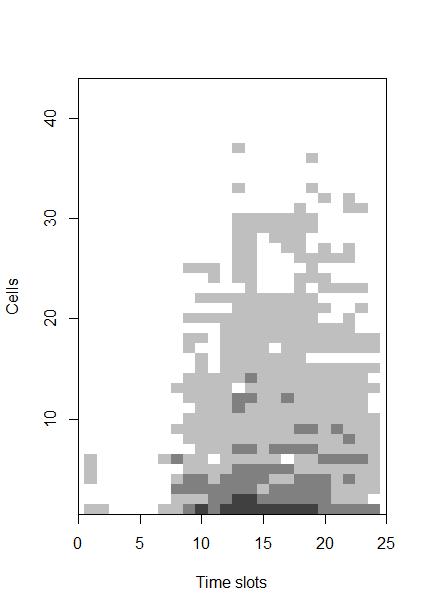 Figure 1
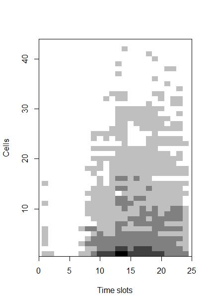 Figure 2
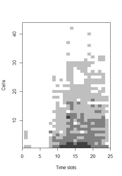 Figure 3
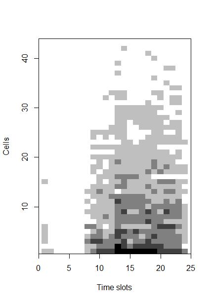 Figure 4
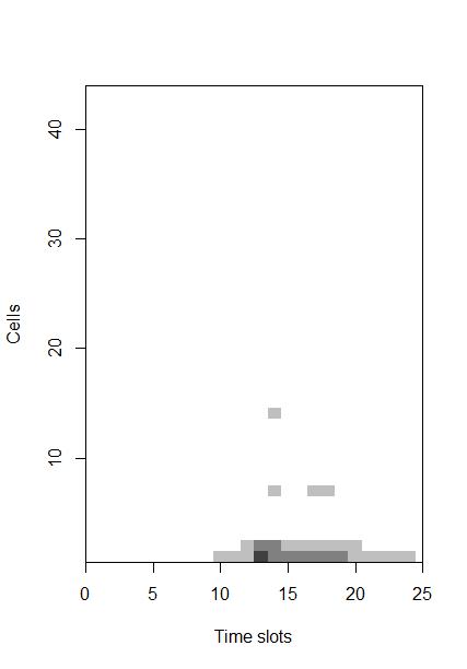 Figure 5
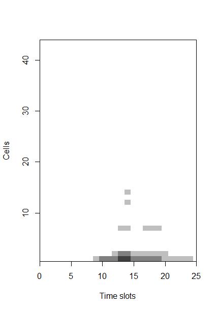 Figure 6
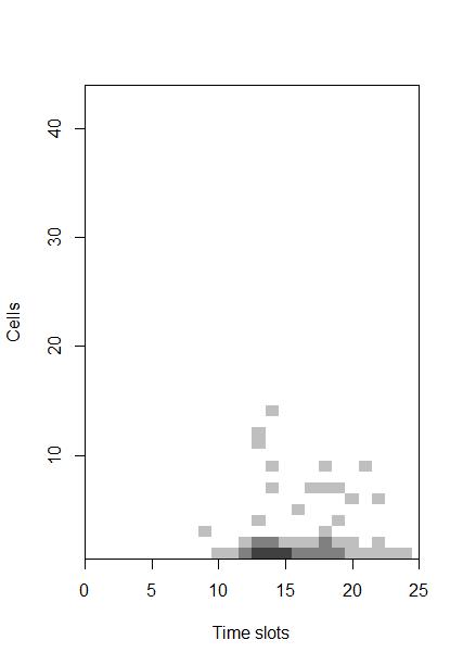 Figure 7
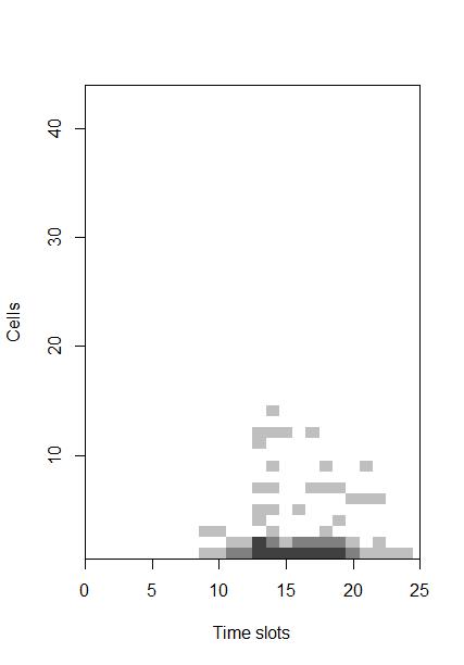 Figure 8
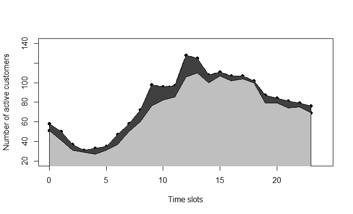 Figure 9
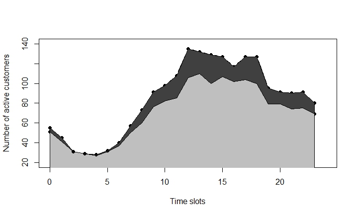 Figure 10
Peer Reviews
No public reviews on file for this paper yet. If you reviewed it on a platform where reviews are public (OpenReview, ICLR, NeurIPS, ICML), you can paste yours below so the community can read it here.
Videos
No videos yet. Explain this paper in a talk, walkthrough, or lecture? Add one.
Taxonomy
TopicsICT Impact and Policies · Auction Theory and Applications · Advanced Queuing Theory Analysis
∎
11institutetext: M. Akian 22institutetext: INRIA, CMAP, Ecole Polytechnique, CNRS
Route de Saclay
91128 Palaiseau Cedex, France
Tel.: +331 69 33 46 39
22email: [email protected] 33institutetext: M. Bouhtou 44institutetext: Orange Labs
44, avenue de la République
92320 Chatillon, France
44email: [email protected] 55institutetext: J.B. Eytard 66institutetext: INRIA, CMAP, Ecole Polytechnique, CNRS
Route de Saclay
91128 Palaiseau Cedex, France
66email: [email protected] 77institutetext: S. Gaubert 88institutetext: INRIA, CMAP, Ecole Polytechnique, CNRS
Route de Saclay
91128 Palaiseau Cedex, France
Tel.: +331 69 33 46 03
88email: [email protected]
Preprint submitted to EURO Journal on Computational Optimization October 31, 2018
A bilevel optimization model for load balancing in mobile networks through price incentives
Marianne Akian
Mustapha Bouhtou
Jean Bernard Eytard
Stéphane Gaubert
Abstract
We propose a model of incentives for data pricing in large mobile networks, in which an operator wishes to balance the number of connections (active users) of different classes of users in the different cells and at different time instants, in order to ensure them a sufficient quality of service. We assume that each user has a given total demand per day for different types of applications, which he may assign to different time slots and locations, depending on his own mobility, on his preferences and on price discounts proposed by the operator. We show that this can be cast as a bilevel programming problem with a special structure allowing us to develop a polynomial time decomposition algorithm suitable for large networks. First, we determine the optimal number of connections (which maximizes a measure of balance); next, we solve an inverse problem and determine the prices generating this traffic. Our results exploit a recently developed application of tropical geometry methods to mixed auction problems, as well as algorithms in discrete convexity (minimization of discrete convex functions in the sense of Murota). We finally present an application on real data provided by Orange and we show the efficiency of the model to reduce the peaks of congestion.
Keywords:
Bilevel programming Mobile data networks Tropical geometry Discrete convexity Graph algorithms
1 Introduction
With the development of new mobile data technologies (3G, 4G), the demand for using the Internet with mobile phones has increased rapidly. Mobile service providers (MSP) have to confront congestion problems in order to guarantee a sufficient quality of service (QoS).
Several approaches have been developed to improve the quality of service, coming from different fields of the telecommunication engineering and economics. For instance, one can refer to Bonald and Feuillet bonald2013network for some models of performance analysis to optimize the network in order to improve the QoS. One of the promising alternatives to solve such problems consists in using efficient pricing schemes in order to encourage customers to shift their mobile data consumption. In maille2006pricing , Maillé and Tuffin describe a mechanism of auctions based on game-theoretic methods for pricing an Internet network, see also maille2014telecommunication . In altman2006pricing , Altman et al. study how to price different services by using a noncooperative game. These different approaches are based on congestion games. In the present work, we are interested in how a MSP can improve the QoS by balancing the traffic in the network. We wish to determine in which locations, and at which time instants, it is relevant to propose price incentives, and to evaluate the influence of these incentives on the quality of service.
This kind of problem belongs to smart data pricing. We refer the reader to the survey of Sen et al. sen2013survey and also to the collection of articles sen2014smart . Finding efficient pricing schemes is a revenue management issue. The first approach consists in usage-based pricing; the prices are fixed monthly by analysing the use of the former months. It is possible to improve this scheme by identifying peak hours and non-peak hours and proposing incentives in non-peak hours in order to decrease the demand at peak hours and to better use the network capacity at non-peak hours. This leads to time-dependent pricing. Such a scheme for mobile data is developed by Ha et al. in ha2012tube . The prices are determined at different time slots and based on the usage of the previous day in order to maximize the utility of the customers and the revenue of the MSP. This pricing scheme was concretely implemented by AT&T, showing the relevance of such a model. In another approach, Tadrous et al. propose a model in which the MSP anticipates peak hours and determines incentives for proactive downloads tadrous2013pricing .
The latter models concern only the time aspects. One must also take into account the spatial aspect in order to optimize the demand between the different locations. In ma2014time , Ma, Liu and Huang present a model depending on time and location of the customers where the MSP proposes prices and optimizes his profit taking into account the utility of the customers.
Here, we assume (as in ma2014time ) that the MSP proposes incentives at different time and places. Then, customers optimize their data consumption by knowing these incentives and the MSP optimizes a measure of the QoS. In this way, we introduce a bilevel model in which the provider proposes incentives in order to balance the traffic in the network and to avoid as much as possible the congestion (high level problem), and customers optimize their own consumption for the given incentives (low level problem).
Bilevel programs have been widely studied, see the surveys of Colson, Marcotte and Savard colson2007overview and of Dempe dempe2003bilevel . They represent an important class of pricing problems in the sense that they model a leader wanting to maximize his profit and proposing prices to some followers who maximize themselves their own utility. Most classes of bilevel programs are known to be NP-hard. Several methods have been introduced to solve such problems. For instance, if the low level program is convex, it can be replaced by its Karush-Kuhn-Tucker optimality conditions and the bilevel problem becomes a classical one-stage optimization problem, which is however generally non convex. If some variables are binary or discrete, and the objective function is linear, the global bilevel problem can be rewritten as a mixed integer program, as in Brotcorne et al. brotcorne2000bilevel .
In the present work, we optimize the consumption of each customer in a large area (large urban agglomeration) during typically one day divided in time slots of one hour, taking into account the different types of customers and of applications that they use. Therefore, we have to confront both with the difficulties inherent to bilevel programming and with the large number of variables (around ). Hence, we need to find polynomial time algorithms, or fast approximate methods, for classes of problems of a very large scale, which, if treated directly, would lead to mixed integer linear or nonlinear programming formulations beyond the capacities of current off-the-shelve solvers.
This motivated us to introduce a different approach, based on tropical geometry. Tropical geometry methods have been recently applied by Baldwin and Klemperer in baldwin2012tropical to an auction problem. This has been further developed by Yu and Tran tran2015product . In these approaches, the response of an agent to a price is represented by a certain polyhedral complex (arrangement of tropical hypersurfaces). This approach is intuitive since it allows one to vizualize geometrically the behavior of the agents: each cell of the complex corresponds to the set of incentives leading to a given response. Then, we vizualize the collective response of a group of customers by “superposing” (refining) the polyhedral complexes attached to every customer in this group. We apply here this idea to represent the response of the low-level optimizers in a bilevel problem. This leads to the following decomposition method: first we compute, among all the admissible consumptions of the customers, the one which maximizes a measure of balance of the network; then, we determine the price incentive which achieves this consumption. In this way, a bilevel problem is reduced to the minimization of a convex function over a certain Minkowski sum of sets. We identify situations in which the latter problem can be solved in polynomial time, by exploiting the discrete convexity results developed by Murota murota2003discrete . In this approach, a critical step is to check the membership of a vector to a certain Minkowski sum of sets of integer points of polytopes. In our present model, these polytopes, which represent the possible consumptions of one customer, have a remarkable combinatorial structure (they are hypersimplices). Exploiting this combinatorial structure, we show that this critical step can be performed quickly, by reduction to a shortest path problem in a graph. This leads to an exact solution method when there is only one type of contract and one type of application sensitive to price incentive, and to a fast approximate method in the general case.
We finally present the application of this model on real data from Orange and show how price incentives can improve the QoS by balancing the number of active customers in an urban agglomeration during one day. These results indicate that a price incentive mechanism can effectively improve the satisfaction of the users by displacing their consumption from the most loaded regions of the space-time domain to less loaded regions.
The paper is organized as follows. In Section 2, we present the bilevel model. In Section 3, we explain how a certain polyhedral complex can be used to represent the user’s responses, and we describe the decomposition method. In Section 4, we deal with the high level problem and identify special cases which are solvable in polynomial time. In Section 5, we develop accelerated algorithms which enable to solve bilevel problems with a large number of customers. In Section 6, we propose a general relaxation method. The application to the instance provided by Orange is presented in Section 7.
The first results of this article (without proofs) were published in the proceedings of the conference WiOpt 2017 eytard2017bilevel .
2 A bilevel model
We consider a time horizon of one day, divided in time slots numbered , and a network divided in different cells numbered . We assume that customers, numbered , are in the network. The customers have different types of contracts and they make requests for different types of applications (web/mail, streaming, download, …). We denote by the set of customers with the contract . A given customer is characterized by the following data. We denote by the position of the customer at each time , so that the sequence represents the trajectory of this customer. We assume that this trajectory is deterministic, so we consider customers with a regular daily mobility (for example, the trip between home and work). We denote by the inclination of a customer to make a request for an application of type at time . We suppose that customer wishes to make a fixed number of requests using the application during the day. We consider a set of time slots in which the customer decides not to consume the application .
We denote by the consumption of the customer for the application at time , setting if is active at time and makes a request of type and otherwise. Therefore, the number of active customers with contract for the application at time and location is given by , where denotes the indicator function, and the total number of active customers at time and location is given by .
We consider the following two-stage model of price incentives. The first stage consists for the operator in announcing a discount at time and location for the customers of contract making requests of type . We consider only nonnegative discounts, so . The second stage models the behavior of customers who modify their consumption by taking the discounts into account. We will assume the preference of a customer of contract for consuming at time becomes , where denotes the sensitivity of customer to price incentives for the application . It corresponds to classical linear utility functions, see e.g. baldwin2012tropical . We also assume that the customers cannot make more than one request at each time, that is , . Therefore, each customer determines his consumptions for the applications, as an optimal solution of the linear program:
Problem 1 (Low-level, customers).
[TABLE]
[TABLE]
Consequently, each price determines the possible individual consumptions for the users with contract , and so the possible cumulated traffic vectors and . The aim of the operator is, through price incentives, to balance the load in the network into the different locations and time slots to improve the quality of service perceived by each customer. We introduce a coefficient relative to the kind of contracts of the different customers in order to favor some classes of premium customers. In lee2005non , Lee et al. suppose that the satisfaction of a customer depends on his perceived throughput, which can be considered as inversely proportional to the number of customers in the cell. Here, we assume that the satisfaction of each customer in the cell is a nonincreasing function of the total number of active customers in the cell , depending on the characteristics of the cell, of the type of application the user wants to do (some applications like streaming need a higher rate than others) and on the type of contract. We also assume that the satisfaction of all the customers with contract using a given application in a given cell is maximal until the number of active customers reaches a certain threshold , then for . After this threshold, the satisfaction decreases until a critical value . We add the constraint to prevent the congestion. For non-real time services like web, mail, download, the satisfaction function can be viewed as a concave function of the throughput, like where denotes the throughput, see Moety et al. moety2016satisfaction . Hence, we will consider that for contents like web, mail and download, , for and for where is a positive parameter depending on the kind of contract of the customer. The more expensive the contract of the customer is, the larger is . We can prove that this function is concave for . For real time services like video streaming, the customers need a more important throughput to ensure a good QoS lee2005non . We will here consider the same type of functions but with replaced by , that is for .
So, the first stage consists in maximizing the global satisfaction function which depends on the vectors and is defined by:
[TABLE]
with . Our final model consists in solving the following bilevel program:
Problem 2 (High-level, provider).
[TABLE]
where , and , , and , the vectors are solutions of Problem 1.
3 A decomposition approach for solving the first model
We will present a decomposition method for solving the previous bilevel problem. In this section, and in the next two ones, we suppose that there is only one kind of application and one kind of contract. This special case is already relevant in applications: it covers the case when, for instance, only the download requests are influenced by price incentives, whereas other requests like streaming or web are fixed. Whereas the analytical results of the present section carry over to the general model, the results of the next two sections (polynomial time solvability) are only valid under these restrictive assumptions. We shall return to the general case in Section 6, developing a fast approximate algorithm for the general model based on the present principles.
In the above special case, the bilevel model can be rewritten:
[TABLE]
where and , and for each the vectors are solutions of the problem:
[TABLE]
[TABLE]
In order to deal more abstractly with the bilevel model, we introduce the notation . Hence, we have if . By defining the set or , we have that implies that . We can then define if and otherwise. Then, we can rewrite each low-level problem as:
[TABLE]
where , and the global bilevel problem becomes:
[TABLE]
with . Notice that the set corresponds to the set of couples such that . It is possible to enumerate all the couples . Let us define and associate each couple to an integer . The quantities , , and can be respectively denoted by , , and . The function and the integer can be respectively denoted by and . It means that for two indices and associated to two couples and with the same , we have and . The low-level problem can be rewritten:
Problem 3 (Abstract low-level problem).
[TABLE]
where and .
The global bilevel problem is:
Problem 4 (Bilevel problem).
[TABLE]
with for all , solution of Problem 3.
Lemma 1.
Suppose that the functions are nonincreasing and concave on . Then, the functions are also concave on .
Proof.
The result comes easily if we suppose that the functions are twice differentiable, because we have:
[TABLE]
We could deduce that the same is true without the differentiability assumption by a density argument, writing a concave function as a pointwise limit of smooth concave functions. However, we prefer to provide the following elementary argument. Consider and . Because is nonincreasing, we have . We have:
[TABLE]
Because of the well-known inequality , we have:
[TABLE]
Then, because is nonincreasing, we have:
[TABLE]
so that:
[TABLE]
and is concave. ∎
3.1 A tropical representation of customers’ response
The lower-level component of our bilevel problem can be studied thanks to tropical techniques. Tropical mathematics refers to the study of the max-plus semifield , that is the set endowed with two laws and defined by and , see bcoq ; itenberg2009tropical ; butkovicbook ; MacLaganSturmfels for background. We first consider the relaxation in which the price vector can take any real value, i.e. . Each customer defines his consumption by solving the problem:
[TABLE]
The map is convex, piecewise affine, and the gradients of its linear parts are integer valued. It can be thought of as a tropical polynomial function in the variable . Indeed, with the tropical notation, we have
[TABLE]
where denotes the th tropical power. In this way, we see that all the monomials of have degree , so that is homogeneous of degree , in the tropical sense. This remark leads to the following lemma:
Lemma 2.
Denote by . Let be a solution of the relaxation of Problem 4. Then, for all , is a solution of the relaxation of Problem 4.
Proof.
Consider a solution of the relaxed problem. Because is homogeneous of degree , we have for all , . In particular:
[TABLE]
Hence, leads to the same repartition of the customers and corresponds also to an optimal solution of the relaxed bilevel problem. ∎
Corollary 1.
The bilevel problem 4 has the same value as its relaxation .
Proof.
Consider a solution of the relaxed problem, and take . Then, we have and solution of the relaxed problem according to Lemma 2. Consequently, is a solution of Problem 4. ∎
By definition, the tropical hypersurface associated to a tropical polynomial function is the nondifferentiability locus of this function. Since the monomial is homogeneous, its associated tropical hypersurface is invariant by the translation by a constant vector. Therefore, it can be represented as a subset of the tropical projective space . The latter is defined as the quotient of by the equivalence relation which identifies two vectors which differ by a constant vector, and it can be identified to by the map
, .
Example 1.
Consider a simple example with time steps (for instance morning, afternoon and evening), (that is ), and for each . The parameters of the customers are
[TABLE]
The tropical polynomial of the first customer is , meaning that this customer has no preference and consumes when the incentive is the best. Its associated tropical hypersurface is a tropical line (since has degree ), so it splits in three different regions corresponding to a choice of the vector among , and , see Figure 2. E.g., the cell labeled by represents a consumption concentrated the morning, induced by a price and .
To study jointly the responses of the five customers, we represent the arrangement of the tropical hypersurfaces associated to the (see Figure 3), with
[TABLE]
Lemma 3 (Corollary of (tran2015product, , §4, Lemma 3.1)).
Each cell of the arrangement of tropical hypersurfaces corresponds to a collection of customers responses and to a unique traffic vector , defined by .
3.2 Decomposition theorem
We next show that the present bilevel problem can be solved by decomposition. We note that the function to optimize for the higher level problem, i.e. the optimization problem of the provider, depends only on . The variables allow one to generate the different possible vectors .
Definition 1.
A vector is said to be feasible if there exists vectors such that and there exists such that for each , .
So, we will characterize the feasible vectors in order to optimize directly the satisfaction function on the set of feasible . We define the relaxation of Problem 4 to the case .
Problem 5 (Bilevel problem with real discounts).
[TABLE]
with and for all , solution of:
[TABLE]
According to Lemma 1, Problem 4 has the same value than the relaxation problem 5. Moreover, according to Lemma 2, if is an optimal solution of Problem 5, then is also an optimal solution of Problem 5 for every . We recall that is a vector defined by . Then, if we find an optimal solution of Problem 5, then with is a solution of Problem 5 such that . Consequently, is a solution of Problem 4. Hence, a solution of Problem 5 (with real discounts) provides a solution of Problem 4 (with nonnegative discounts). In the sequel, we will study the bilevel problem 5.
Most of the following results are applications of classical notions of convex analysis which can be found in rockafellar1970convex . It is convenient to introduce the convex characteristic function of a set , defined by if , and otherwise. If is a convex set, then is a convex function. We define also for every the polytope as the convex hull of , together with the convex function defined by .
Lemma 4.
* and and is exactly the set of vertices of .*
Proof.
Let us define the polytope and . Clearly, . Then, .
Consider a point of which is not in . There exists an index such that . In particular . However, . So, there exists another index such that . Hence, there exists such that the points ans defined by:
[TABLE]
are in . Because with and , is not a vertex of . Consequently, the set of vertices of is included in . Because is the convex hull of its vertices, we have .
The polytope is such that , with if and otherwise, and . Then, because is a totally unimodular matrix, the vertices of are exactly its integer points, that is . ∎
Corollary 2.
The value of each low level problem 3 is the value of the Legendre-Fenchel transform of at point , i.e. .
Proof.
The vertices of are . Hence:
[TABLE]
∎
We want to characterize the feasible vectors. We have first the following result.
Lemma 5.
Let be a real vector. Then, there exists and such that and for every , if and only if .
Proof.
Such vectors belong to , so .
Let and . A vector is such that if and only if , where denotes the subdifferential of the convex function . Then, a vector if and only if . By (rockafellar1970convex, , Th. 23.8), , where is the inf-convolution of the functions .
Let be a real vector. Then, there exists and such that and for every , if and only if , or equivalenty (because is convex), that is if and only if . The function is polyhedral (as the inf-convolution of polyhedral convex functions) and it is finite at every point in . So, is a non-empty polyhedral convex set (rockafellar1970convex, , Th. 23.10). The result comes straightforwardly. ∎
It is now possible to characterize the feasible vectors.
Lemma 6.
A vector is feasible if and only if .
Proof.
According to Definition 1, a vector is feasible if and only if there exists and vectors such that and . As a consequence of Lemma 4, . Then, by Lemma 5, a vector is feasible if and only if . We have now to prove . Because , the inclusion is obvious. Conversely, consider . Then, the set is a non-empty polytope. A vector belongs to if it satisfies the following constraints:
[TABLE]
, that is , with such that for every , and and defined by:
[TABLE]
By Poincaré’s lemma, is totally unimodular. In particular, the extreme points of are integer. Then, there exists with for every , such that . ∎
Each vector can be written as sum of vectors for such that there exists with . In order to determine such vectors , we have the following lemma:
Lemma 7.
Let with . The following assertions are equivalent:
There exists such that for each , . 2. 2.
The vectors realize the minimum in the inf-convolution , i.e.
[TABLE]
.
Proof.
(1) (2) : We have for every :
[TABLE]
By summing those equalities, we have:
[TABLE]
By considering only the vectors such that , we can write which is exactly the second assertion.
(2) (1): The set is non-empty. Consider , that is . We can write:
[TABLE]
So:
[TABLE]
Consequently, if one is not an optimal solution of the low-level problem, the previous equality cannot be true. ∎
The high-level problem of Problem 5 consists in maximizing a function depending only on a vector which has to be a feasible vector. It is now possible to write the main theorem of this section, which establishes a decomposition method for solving Problem 5.
Theorem 3.1.
(Decomposition)* The bilevel problem 5 can be solved as follows:*
Find an optimal solution to the high level problem with unknown :
[TABLE] 2. 2.
Find vectors solutions of the following problem:
[TABLE] 3. 3.
Find a vector such that , is a solution of the low level problem.
Proof.
The bilevel programming problem 5 can be rewritten subject to . According to Lemma 6, is feasible if and only if . So, a necessary condition for a vector to be an optimal solution of the bilevel problem is that for every , there exists such that is an optimal solution of the problem:
[TABLE]
After finding , it is possible to find by solving the inf-convolution problem as a consequence of Lemma 7. Because is equivalent to , each point of is an optimal solution of the bilevel problem.
∎
The second step of this theorem consists in solving a linear program. We next show that the third step reduces to a linear feasibility problem.
Lemma 8.
Let be a feasible vector and () be vectors such that and . Then, the set of vectors such that , is non-empty and is the polytope defined by the following inequalities:
[TABLE]
Proof.
According to Lemma 7, there exists . Hence, we have , .
Consider indices with , , and the vector defined by , and . We verify easily , so that the condition , which can be rewritten , is satisfied.
Moreover, this condition is sufficient. Consider such that with , , we have . Consider . By definition of , the quantity corresponds to the sum of coordinates of for which the index is not in . Hence,
[TABLE]
because of the lemma hypothesis and because
∎
For every , the latter inequalities define a polytope, and we have to find in the intersection of all these polytopes.
4 A first algorithm
In this section, we explain how the decomposition method provided by Theorem 3.1 leads to a polynomial time algorithm for solving Problem 5. We will use some elements of discrete convexity developed by Danilov, Koshevoy danilov2004discrete and Murota murota2003discrete , that we recall first. We next explain how to solve Problem 5.
An integer set is -convex (murota2003discrete, , Ch. 4, p.101) if such that such that , and , where is the -th vector of the canonical basis in .
Lemma 9.
The feasible domain of the high-level program
[TABLE]
is a -convex set of .
Proof.
We can check easily that , the set is -convex. Taking two different vectors and in , there exist such that and . These indices do not belong to . The vectors and have coordinates in with a sum equal to and all coordinates in equal to 0.
It is known that a Minkowski sum of -convex sets is -convex (murota2003discrete, , Th. 4.23, p.115), and so the set is -convex.
Finally, consider two vectors and of . They belong to , so for each with , we can find with such that and are in . The -th coordinate of is and the -th coordinate of is . So and similarly , which proves the -convexity of .
∎
A function is -convex (murota2003discrete, , ch. 6.1, p.133) if such that and are finite real values, such that , such that and the following condition holds true:
[TABLE]
A function is -concave if is -convex. It follows from this definition that if is a -convex set, then is a -convex function (we recall that is defined by if and otherwise). An important property of -convex functions is that local optimality guarantees global optimality (murota2003discrete, , Th. 6.26, p.148) in the following sense. Let be a -convex function and . Then if and only if .
According to Theorem 3.1, we have to solve , where is a separable concave function, and is the -convex set introduced in Lemma 9. The function is -concave (murota2003discrete, , Th. 6.13.(4), p.143). Then, we have the following result as a direct consequence of (murota2003discrete, , Th. 6.26, p.148) :
Theorem 4.1.
Let . Then, is a maximum point of over if and only if such that .
Moreover, Murota (murota2003discrete , ch.10, p.281) gives an algorithm which runs in pseudo-polynomial time to minimize -convex functions (see Algorithm 1).
By adding a priority rule in Step 2 of Algorithm 1 in the case where is not reduced to a single point, a global minimizer of is obtained by Algorithm 1in pseudo-polynomial time.
Proposition 1 (murota2003discrete , Prop.10.2).
Assume that is bounded. Let be the number of arithmetic operations needed to evaluate and . Then, if a vector in is given, Algorithm 1 finds a global minimizer of in time.
However, the minimization of a -convex function can be achieved in polynomial time.
Proposition 2 (murota2003discrete , Prop.10.4).
Assume that is bounded. Let be the number of arithmetic operations needed to evaluate and . Then, if a vector in is given, a global minimizer of can be found in time.
The different algorithms developed by Murota (murota2003discrete, , Section 10.1) provide a minimizer of a -convex function in polynomial time, if an initial point is given and if the domain of the function is bounded. Whereas it is trivial to find a vector of such that or a vector belonging to , it is not obvious to find one satisfying both conditions. In fact, such a point can be obtained by solving the minimization problem:
[TABLE]
The condition is equivalent to if is non-empty. The function is separable convex. Then, the function is -convex according to (murota2003discrete, , Th. 6.13.(4), p.148). Because is bounded and a point in can be obtained in operations by summing vectors taken in each set , it is possible to find a point in polynomial time, by Proposition 2.
We can finally write the following result about the complexity of the decomposition method given by Theorem 3.1.
Theorem 4.2.
Let , for every , and . An optimal solution of Problem 5 can be obtained in arithmetic operations, where is the input size of the bilevel problem.
Proof.
The first step of Theorem 3.1 is a maximization of a -concave function over a bounded domain . Finding a point in can be done by solving the -convex minimization problem:
[TABLE]
The domain of the function is . We define by:
[TABLE]
For every , the entries of are sum of binary values. Then, . We have to estimate the number of operations needed to evaluate the function . The function can be evaluated in operations. As a consequence of Lemma 6 and Lemma 7, . Hence, for any vector , the conditions is equivalent to . A vector belongs to if there exists for every a vector such that . Hence, to know whether belongs to or not is a linear feasibility problem in dimension , It can be solved in arithmetic operations by an interior point method (renegar1988polynomial ). Here is the input size of the linear program. Consequently, , and a point in can be obtained in by Theorem 2.
After obtaining a point in , the first step of Theorem 3.1 consists in solving the -concave maximization problem:
[TABLE]
The domain of the function is bounded and equal to . We define by:
[TABLE]
For every , the entries of are sum of binary values. Then, for every , we have Then, , with . The number of operations needed to evaluate the function is like previously. Hence, a point can be obtained in by Theorem 2.
According to the proof of Lemma 6, the second step of Theorem 3.1 is a linear program in dimension . In fact, we have:
[TABLE]
and the extreme points of the polyhedron defined by:
[TABLE]
are integer. Hence, the second step of Theorem 3.1 can be solved in arithmetic operations.
The third step of Theorem 3.1 is a linear program in variables. For some , the constraints of this program are:
[TABLE]
For every , the number of entries of equal to is , and the number of entries of equal to [math] and which do not belong to is . Hence, the number of inequality constraints of this linear program is . Hence, a solution of this linear program can be found in by interior-point methods. ∎
5 A faster algorithm for solving the bilevel problem
5.1 A polynomial time algorithm for the bilevel problem
Algorithm 1 can be applied to solve problem (6) of Theorem 3.1, that is maximizing the -concave function , or equivalently minimizing the -convex function .
Step 1 consists in finding an initial vector . As explained in Section 4, this can be done by solving a -convex minimization problem. Another approach consists in replacing the function by , where is an integer. If , then . If is sufficiently large, then if , and the maximum of the function is attained for . Moreover is separable convex, then is -concave according to (murota2003discrete, , Th. 6.13.(4), p.148). Then, both problems and are equivalent, and we can apply Algorithm 1 to solve the problem . An initial point is obtained by taking any point in .
We need first part is to determine the number of operations to evaluate . Because the different functions are known, we have to determine the number of operations to decide whether a vector belongs to or not. More precisely, the different evaluations of are done in Step 2. Hence, the question is the following: given a vector , how many operations are needed to check whether (for ) belongs to . We next show that this problem can be studied as a shortest path problem in a graph. Consider and let us define for such that , that is an optimal decomposition of in Theorem 3.1. For each and , we define by the following quantity: if and , and otherwise. Then, we define for each , . We consider the oriented valuated graph where the set of vertices and there is an oriented edge between each vertices of value .
Theorem 5.1.
Let . Suppose that there exists a path in with finite valuation between the vertices . Then . Moreover, there are no negative cycles and there is a shortest path between and . Let be any sequence such that , and let be a shortest path between and . Let also be any sequence such that for all . Let us finally define the vectors , such that for each and for each . Then, .
Proof.
By Lemma 6 and 7, we know that if and only if there exists vectors such that with each and . We consider with each . Hence, is equal to:
[TABLE]
We have . When describes , the possible are the vectors with the following properties:
[TABLE]
Hence, , where is such that . Consequently, can be written as a sum of for certain . Because of the condition , we have , with the notations introduced in Theorem 5.1.
Consider now the graph defined in Theorem 5.1. If there exists a path between and , then its value can be written (with the convention and ). By defining if and for , the value of the path is equal to . Because , we have and . Then, each . Consequently, the value is finite and . Moreover, the value corresponds to the minimal values of the path between and in , that is the shortest path. Hence, if the value of the shortest path is , we have , with defined as in the statement of Theorem 5.1. Moreover, we can prove that there exists no cycle with negative weight in this graph. Suppose that such a cycle exists. It can be written . For all , we have and . We consider for the vectors defined by , and for . We have and so which refutes the optimality of the vectors in the definition of . ∎
Example 2.
We consider the cell (a) of Figure 3. We build the graph associated to (see Figure 4).
Consider . The shortest path in is with . Then, according to Theorem 5.1, the optimal decomposition of is , , , and .
Thanks to Theorem 5.1, if we know that a vector belongs to , it is possible to check whether a vector belongs to by checking if there exists a path between and in the graph . Generally, has vertices and edges. From each vertex , it is possible to find if there exists a path between and by using a depth-first or breadth first search algorithm in operations. Consequently, the number of operations needed to evaluate is .
According to Theorem 5.1, by checking if , we obtain the optimal decomposition of such that by solving a shortest path problem between two vertices. This can be done in operations thanks to Ford-Bellman algorithm (bellman1958routing , ford1956network ), because the graph has vertices and at most edges. Hence, according to Theorem 3.1, it suffices to solve the bilevel problem 5 to solve the linear feasibility problem of Lemma 8. Moreover, this problem can also be viewed as a shortest path problem in , according to the following result.
Theorem 5.2.
Consider vectors for each such that, if we define , we have . Consider the graph associated to . Consider an index . Let be any real scalar such that and let us modify such that for all with and , we have . Let us define a vector by and for each with , is the length of the shortest path between and in . Then, for sufficiently large and for each , .
Proof.
According to Lemma 8, a vector is such that for every ,
[TABLE]
if and only if the following inequalities are satisfied:
[TABLE]
Consider such a vector . Consider also the graph associated to The previous inequalities can be rewritten , or equivalently : . For each , is also a solution. Consequently, it is possible to fix a coordinate to [math]. Take a coordinate such that . Consider such that and modify the graph as in the statement of the theorem. Consider an elementary cycle (that is a cycle containing no smaller cycle) of the modified graph. The cycle has no more than edges. Suppose that exactly edges have a modified weight, with . If , then no edge has a modified weight, and this cycle is a cycle of . So, its weight is nonnegative. If , then the total weight of the cycle is bigger than . Consequently, the modified graph has no negative cycles.
For each , with , there exists a path between and . Let us define such that and for each with , corresponds to the length of the shortest path between and . Consider . Then is the length of a path between and defined as the concatenation of the shortest path between and and the edge . So . Hence, according to Lemma 8, we have for each , . ∎
These different results lead to Algorithm 2 to solve the bilevel problem 5. First, we have to find an initial point in , with its optimal decomposition . We can calculate for each and for each the value , store them, and then define the graph associated to . Hence, with a graph search algorithm, we know for each whether or not, and can calculate for each and find . By finding the shortest path between and in , we obtain the optimal decomposition . Like in Algorithm 1, if , then is the maximum value of over . Else, we take . For all the indices such that , we evaluate the new value of and we define the graph associated to and restart the algorithm. Notice that the number of indices such that is bounded by the length of the shortest path in ; it means that this number is less than . After finding the optimal and having its optimal decomposition , we can redefine the graph associated to and return an optimal defines as in the statement of Theorem 5.2.
Algorithm 2 can be written as follows. We take in input a function GraphSearch, which associate to a graph (defined by the weight vector of its edges) a Boolean vector such that if there is an edge between and and [math] otherwise. We also take a function ShortestPath, which associate to a graph (also defined by the weight vector ) and two vertices and , the value of the shortest path and a vector with the indices of this shortest path. Finally, we consider the function ShortestPath2, which associate to and a vertex a vector corresponding to the values of the shortest path between and all other vertices in . For much ease, we denote by the function .
Note that the pseudo-polynomial time bound for Murota’s greedy algorithm 1 given by Proposition 1 leads in this special case to a polynomial time bound, as explained in the following result.
Theorem 5.3.
Let us define , for each (that is the number of possible non-zero entries of the vectors of and . Algorithm 2 returns a global optimizer with a time complexity of and a space complexity of .
Proof.
The vector returned by the algorithm is a global optimizer according to Algorithm 1 and Theorem 5.1. The initialization consists in taking vectors in each and in adding them; it can be done in operations. Then, to define the graph , we have to calculate for each and each , and to store the values. Let us define for each . For each , we have , and there are precisely coordinates of equal to 1 for each . Then, for each , there are exactly finite values of to store. Then, by defining , we need operations to define and . The function needs operations by a depth-first or breadth-first algorithm to know if there is a path between and . The function needs also operations to calculate the shortest path between and with Ford-Bellman algorithm. The length of the path is bounded by . Consequently, there is less than vectors which have to be updated; and then less than values to update. operations are needed to calculate the new values of and . So, the number of operations in each step of the "while" loop is . The number of iterations of the loop is the same as in Algorithm 1, and is bounded by where . For each , we have:
[TABLE]
by defining . Finally, to find the optimal , operations are needed to find , and operations are needed to evaluate the function by using again the Ford-Bellman algorithm. Step 7 consists in calculating the shortest path between a vertex and the other ones in a graph with vertices and edges. Then, Step 7 can be obtained in thanks to Ford-Bellman algorithm. Hence, the global time complexity of Algorithm 2 is and space complexity is . ∎
Notice that for each , and . Then and . Therefore, the time complexity of Algorithm 2 is in the worst case, whereas the space complexity is .
Example 3.
Consider again Example 1 together with the concave function defined by
[TABLE]
We suppose that . Hence, we can prove that and . First, we want to solve . We start from , a feasible point. Following Algorithm 1, we compute and which is a minimizer. We take . Now, we solve . We obtain , , , , . Applying Lemma 8, we obtain the linear inequalities , and . In particular, is an optimal solution.
5.2 A particular case : theory of majorization
Algorithm 2 can be accelerated in the particular case , that is .
As previously, an important step of the maximization of the function consists in being able to know whether a point belongs to or not. In this particular case, we can use the majorization order olkin1979inequalities . For every , denote by the coordinates of arranged in nonincreasing order. A vector is said to be majorized by another vector , denoted , if and , .
We have the following result.
Theorem 5.4 (Gale-Ryser , see (olkin1979inequalities, , Th. 7.C.1)).
Let and be two integer vectors with nonnegative values. Let defined by . Then, the following assertions are equivalent:
** 2. 2.
There exists a matrix such that for each , , and
Corollary 3.
Denoting by the vector with exactly and by , for , we have .
Proof.
A vector belongs to if and only if for each , corresponds to the sum of the coefficients of the -th column of a matrix of size with coefficients in and such that the sum of the coefficients of the -th line is . We conclude by 5.4. ∎
Example 4.
Consider Example 1. We have , and . So is feasible iff verifies .
Like for Algorithm 2, we need to know for a given whether for each . It is possible to answer to this question in polynomial time in by sorting for each and by checking the condition . The time complexity of such a procedure is . However, it can be accelerated thanks to the following result.
Lemma 10.
Let , and . Let be the function defined on such that , is the sum of the largest values of the coordinates of . Suppose finally that is the -th largest value of the coordinates of (if , then we suppose that the -th largest value of is strictly bigger than ), and that is the -th largest value of the coordinates of (if , then we suppose that the -th largest value of is strictly smaller than ). Then if and only if and, either or .
Proof.
Suppose . Then and . Moreover, suppose . Then, and . Then, .
Conversely, if , then all the coordinates of are nonnegative integers. If , then we easily see that . So and . Suppose that . Because we suppose that the -th largest value of is strictly bigger than , then . We also suppose that . The -th largest value of is strictly bigger than , so it is bigger than . Consequently, we have for all , (because ). Moreover, . Because the -th larger coordinate of is strictly smaller than , then it is smaller than and we have and , . Hence, and . ∎
To solve the bilevel problem 5 in this specific case, we need to find such that . In Algorithm 2, such vectors are found in the same time as . Then, to accelerate Algorithm 2, we need to be able to solve this problem rapidly. In particular, to use a classical linear programming approach leads to a time complexity, which is not acceptable. The problem to solve can be written:
Problem 6.
[TABLE]
We already mentioned in the proof of Theorem 5.4 that the constraints of this linear program can be written , where is a totally unimodular matrix. Therefore, the value of this problem is equal to the value of its continuous relaxation. Moreover, it can be interpreted as a minimum cost flow problem (see (schrijver2003combinatorial, , Ch. 12) for background). We define a bipartite graphs with vertices and , and edges between each and each . Each vertex has an incoming flow equal to , whereas each vertex has an outgoing flow equal to . Moreover, the capacity of each edge is , meaning that each flow satisfies , and a cost is associated to each edge. Hence, the problem consists in finding the flow minimizing the total cost in this graph. Plenty of algorithms exist to solve such a problem. In our case, we have . According to Theorem 5.3, Algorithm 2 needs operations to solve Problem 5. Notice that . Therefore, in order to accelerate Algorithm 2 in the studied case, we need an algorithm solving the flow problem with a complexity depending on in with .
We can interpret the minimum cost flow problem as a minimum cost circulation problem, as presented in (schrijver2003combinatorial, , Ch. 12). We introduce a sink . We define an edge between each and of cost equal to [math], with a lower-bound for the flow equal to and a capacity of . We also define an edge between and each of cost equal to [math], with a lower-bound for the flow equal to and a capacity of . Such a graph is represented on Figure 5.
Such a graph has vertices and edges. The sum of the capacities of the different edges is . In (gabow1989faster, , Sec. 3.3), an algorithm is proposed to solve such a problem. Different complexity bounds of such an algorithm are given in (gabow1989faster, , Th. 3.5). In the case , the optimal vectors can be found in .
We can now write an algorithm for solving the bilevel problem in this specific case. We need first to calculate , where is defined as in the statement of Theorem 5.4, and to find an initial point . We apply the same method as in Algorithm 1. In order to calculate for each , we sort the coordinate of in the decreasing order, and we use Lemma 10 to decide whether for all . We use the same loop as in Algorithm 1 to compute an such that is the maximal value of over . Then, we solve the minimum cost flow problem 6, as described previously, to find the optimal and then we use Lemma 5.2 to determine an optimal . It leads to Algorithm 3. The function associates to a vector a couple , where is a permutation of such that and is such that for each . The function is defined by . The function associates to the different vectors the vectors solving the minimum cost flow problem 6. The functions and are defined as for Algorithm 2.
Theorem 5.5.
Let us define , , for each and . Algorithm 3 is correct and returns a global optimizer in time and space.
Proof.
According to Theorem 3.1, Theorem 5.4, Lemma 10 and Algorithm 1, this algorithm returns an optimal solution of the high-level problem and an optimal discount vector . Similarly as in the proof of Algorithm 2, the number of calls of the "while" loop is bounded by . The function needs time and space operations. operations are needed to evaluate the vector , then the global time complexity of the "while" loop is whereas the space complexity is . Then, the optimal vectors can be obtained in time and space. By calculating only the finite values of (which are not necessary stored here), the number of operations needed to determine each and is , with and for each , . We need only space to store the values and . Finally, the vector can be found by using the Ford-Bellman algorithm in a graph of vertices and edges, that is in time complexity of . ∎
In the worst case, we have and . Then, the time complexity of Algorithm 3 is If the number of bits needed to write is polynomial in and if , then Algorithm 3 is faster than Algorithm 2. We finally notice that a minimum cost flow problem is strongly polynomial time solvable, and it is then possible to adapt Algorithm 3 to return an optimal in strongly polynomial time. However, Algorithm 3 does not go faster than Algorithm 2 in this case.
6 The general algorithm
In this section, we come back to the general bilevel problem 2 proposed in Section 2, and extend Algorithm 2 to it. In the low level problem of each customer, the consumptions for different contents verify the constraints , and . We make the assumption that for each customer , the sets of possible instants at which this customer makes a request for the different applications are disjoint, meaning that for any two applications , the complements of and in have an empty intersection. Then the constraint is automatically verified and the low-level problem of each customer can be separated into different optimization problems corresponding to the consumption vector of each customer for each application . Each of these problems takes the following form:
Problem 7.
[TABLE]
[TABLE]
We denote by the feasible set of this problem. The above assumption (that the complements of and have an empty intersection) is relevant in particular if only one kind of application is sensitive to price incentives. For instance, requests for downloading data can be anticipated (see tadrous2013pricing ) and it makes sense to assume that customers are only sensitive to incentives for this kind of contents. In this case, the assumption means that customers wanting to download data can shift their consumption only at instants when they do not request another kind of content.
Moreover, under this assumption, the decomposition theorem is still valid and Problem 2 can be solved with the following method:
Theorem 6.1 (Decomposition (general case)).
The bilevel problem 2 can be solved as follows:
Find an optimal solution to the high level problem with unknown for each , :
Problem 8.
[TABLE] 2. 2.
For each and , find vectors solutions of the following problem:
[TABLE] 3. 3.
Find for each and a vector such that ,
[TABLE]
.
Proof.
The different problems corresponding for each , for each and for each to Problem 7 are independent. Thus, according to Lemma 6, the global bilevel program consists in solving Problem 8. Moreover, the optimal decomposition of and the optimal price vector are totally independent for each and . Then, the proof of the last two parts in the theorem is the same as in Theorem 3.1. ∎
The last two parts of Theorem 6.1 are independent for each and . Thus, they can be solved similarly as in the case of one kind of application and one kind of contracts, studied in Section 3. We need to solve Problem 8. The function to optimize is separable (it can be written as a sum of function depending only of one coordinate), but these functions are not concave in . However, because each function is concave nonincreasing and each is positive, we notice that , the function which sends to is still concave. Consequently, the function to optimize in Problem 8 is -concave in each vector considered separately, the other one being fixed. This leads to a block descent method, in which we use the same scheme as in Algorithm 1, successively, to maximize the objective function over every vector . We denote by the objective function of the high-level problem. We consider for each a vector . For each couple taken successively, we find belonging to:
[TABLE]
If , then the algorithm stops and returns . Otherwise, we take for each , and begin again. Consequently, Algorithm 2 can be modified to solve the bilevel problem 6 in the general case. It leads to Algorithm 4. The function , and are the same as for Algorithm 2. The function is here defined by:
[TABLE]
with .
Because the objective function of Problem 8 is not -convex in , we have no guarantee of convergence of Algorithm 4 to a global optimal of the function . However, we can characterize the nature of the optimum returned by Algorithm 4. In order to estimate the complexity of Algorithm 4, we define the function by:
[TABLE]
If for each we have , then . Thus, we have
[TABLE]
. Because the set is finite, we can define the value by:
[TABLE]
because has not a constant value.
Theorem 6.2.
Let us define . Let us also define , for each and (that is the number of possible non-zero coordinates of the vectors of and . Algorithm 4 terminates in time and space, and returns vectors and such that :
[TABLE]
Proof.
Algorithm 4 continues while the value is strictly larger than . Because the set is finite, the algorithm terminates. When it stops, the vector is such that :
[TABLE]
For each , the function is -concave. The statement of the theorem comes straightforwardly from the equivalence between local and global optimality for -concave functions.
Algorithm 4 differs from Algorithm 2 by the different applications and kind of contracts and by the number of iterations of the loop. The set of customers is split following the different kind of contracts . Thus, we have to define the parameters for each and and the global space complexity becomes . The number of iterations of the loop can be estimated with a pseudo-polynomial bound. The algorithm continues while . Then, the new value of is . Consequently, at each iteration of the loop, the value of increases of at least until the algorithm stops. The finite values of are nonnegative, and an upper bound is because each function takes values between [math] and . In each loop, the number of operations is to calculate the new values of and to solve a shortest path problem for each and in the graph with nodes corresponding to all couples in and edges with values between vertices . ∎
7 Experimental results
We consider an application based on real data provided by Orange. It involves the data consumptions in an area of cells, during one day divided in time slots of one hour, that is time slots. We will focus here our study on price incentives only for download contents. During this day, a number of more than customers make some requests for downloading data in this area and we are interested in balancing the number of active customers in the network. Even though they are insensitive to price incentives, other kind of requests (web, mail, etc.) have to be satisfied and they are taken into account in the high level optimization problem. We consider two classes of users: standard and premium customers. The premium ones demand a better quality of service. Hence, they are less satisfied than the standard customers if they share their cell with a given number of active customers. We therefore define the satisfaction function as in Section 2. The provider wants to favor the premium customers. Hence, we take for the latter ones and for the standard customers, in the high-level optimization problem. We also assume that the premium customers are less sensitive to the incentives, and thus take for all standard customers and for all premium customers in the low-level problem 1. We estimate very simply the parameters . We take when the customer consumes download at time without incentives, when he does not make any request without incentives but makes a request for download at times or (we assume he could shift his consumption of one hour) and otherwise.
We solve the bilevel problem using Algorithm 4, implemented in Scilab. The computation took 9526 seconds on a single core of an Intel i5-4690 processor @ 3.5 GHz.
On Figures 6– 9, we show the evolution of the satisfaction of different kind of customers for different kind of contents without and with incentives. These results show that price incentives have an effective influence on the load, especially in the most loaded cells (the number of black regions in the space-time coordinates, in which the unsatisfaction of the users is critical, is considerably reduced). Moreover, Figure 10 reveals that the consumption of users is not only moved in time, but also in space: not only some consumption is moved from the peak hour to the night (off peak), but the surface of the dark grey region, representing the total download consumption in the cell over the whole day, is decreased, indicating that some part of the consumption has been shifted to other cells.
8 Conclusion
We presented here a bilevel model for price incentives in data mobile networks. We solved this problem by a decomposition method based on discrete convexity and tropical geometry. We finally applied our results to real data. In further work, we shall consider more general models: unfixed number of requests, nonlinear preferences of the customers, satisfaction functions of the provider taking into account the profit. Stochastic models shall also be considered in particular to take into account the partial information of the provider about the customers preferences and trajectories.
9 Acknowledgments
We thank the reviewers of our earlier work eytard2017bilevel for their remarks and comments. We also thank Orange for providing us real data for our experimental results.
The reference list from the paper itself. Each links out to its DOI / PubMed record.
- 1(1) Altman, E., Barman, D., El Azouzi, R., Ros, D., Tuffin, B.: Pricing differentiated services: A game-theoretic approach. Computer Networks 50 (7), 982–1002 (2006)
- 2(2) Baccelli, F., Cohen, G., Olsder, G., Quadrat, J.: Synchronization and Linearity. Wiley (1992)
- 3(3) Baldwin, E., Klemperer, P.: Tropical geometry to analyse demand. Tech. rep., Working paper, Oxford University (2012)
- 4(4) Bellman, R.: On a routing problem. Quarterly of applied mathematics 16 (1), 87–90 (1958)
- 5(5) Bonald, T., Feuillet, M.: Network performance analysis. John Wiley & Sons (2013)
- 6(6) Brotcorne, L., Labbé, M., Marcotte, P., Savard, G.: A bilevel model and solution algorithm for a freight tariff-setting problem. Transportation Science 34 (3), 289–302 (2000)
- 7(7) Butkovič, P.: Max-linear systems : theory and algorithms. Springer monographs in mathematics. Springer (2010)
- 8(8) Colson, B., Marcotte, P., Savard, G.: An overview of bilevel optimization. Annals of operations research 153 (1), 235–256 (2007)