Optimal VWAP execution under transient price impact
Alexander Barzykin, Fabrizio Lillo

TL;DR
This paper derives explicit solutions for optimal VWAP trading strategies considering linear, transient market impact, extending previous models to more general trading intervals and revealing that optimal strategies can involve both buying and selling.
Contribution
It introduces a comprehensive model for optimal VWAP execution with transient impact, encompassing various benchmark cases and providing explicit solutions for risk-averse investors.
Findings
Explicit solutions for continuous and discrete time models.
Optimal strategies may involve both buying and selling.
Contrasts with Implementation Shortfall where only one direction is optimal.
Abstract
We solve the problem of optimal liquidation with volume weighted average price (VWAP) benchmark when the market impact is linear and transient. Our setting is indeed more general as it considers the case when the trading interval is not necessarily coincident with the benchmark interval: Implementation Shortfall and Target Close execution are shown to be particular cases of our setting. We find explicit solutions in continuous and discrete time considering risk averse investors having a CARA utility function. Finally, we show that, contrary to what is observed for Implementation Shortfall, the optimal VWAP solution contains both buy and sell trades also when the decay kernel is convex.
Click any figure to enlarge with its caption.
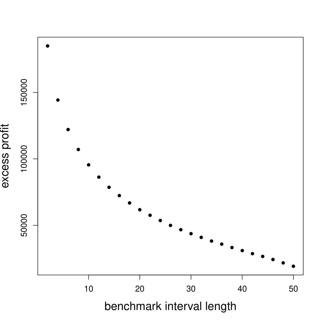 Figure 1
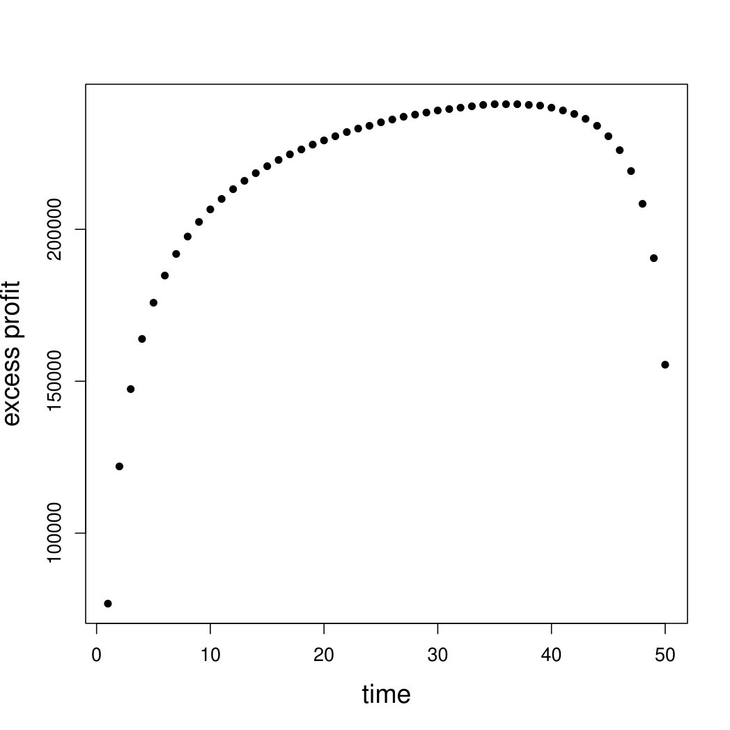 Figure 2
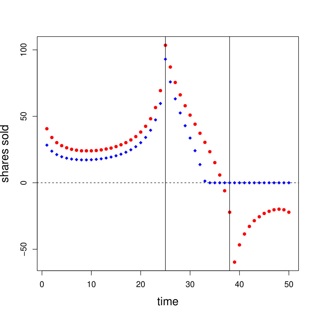 Figure 3
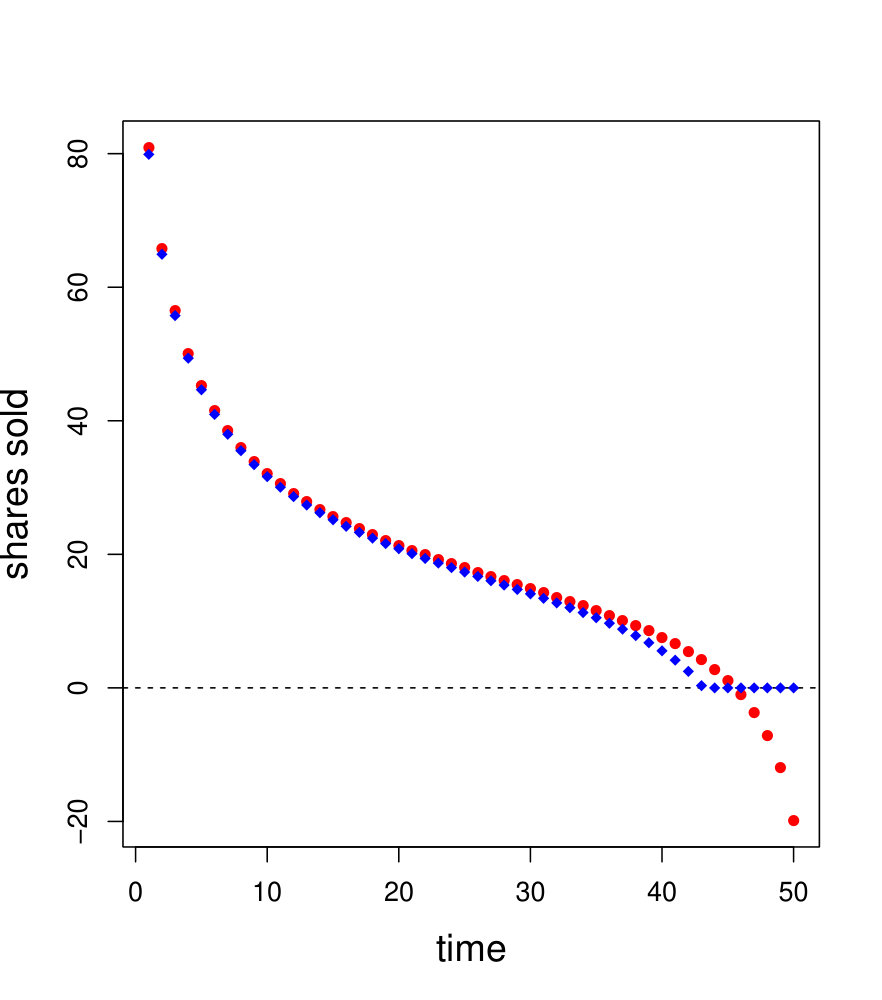 Figure 4
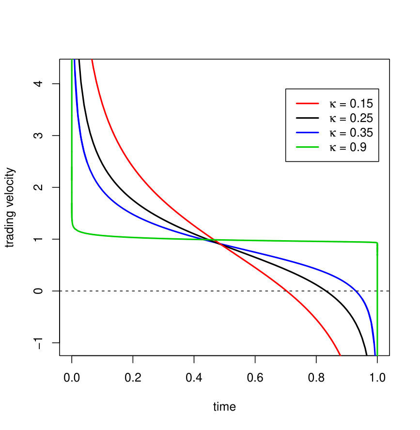 Figure 5
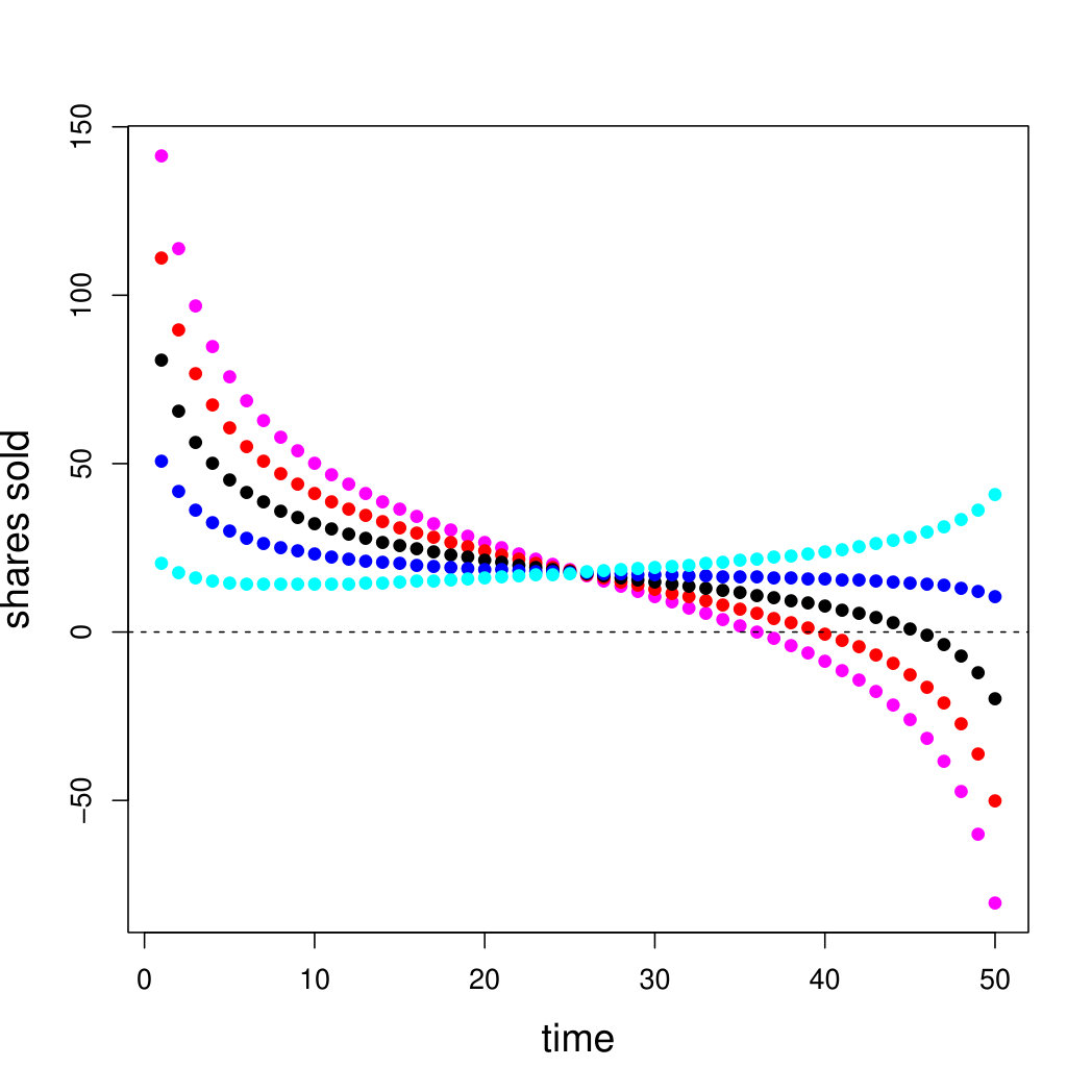 Figure 6
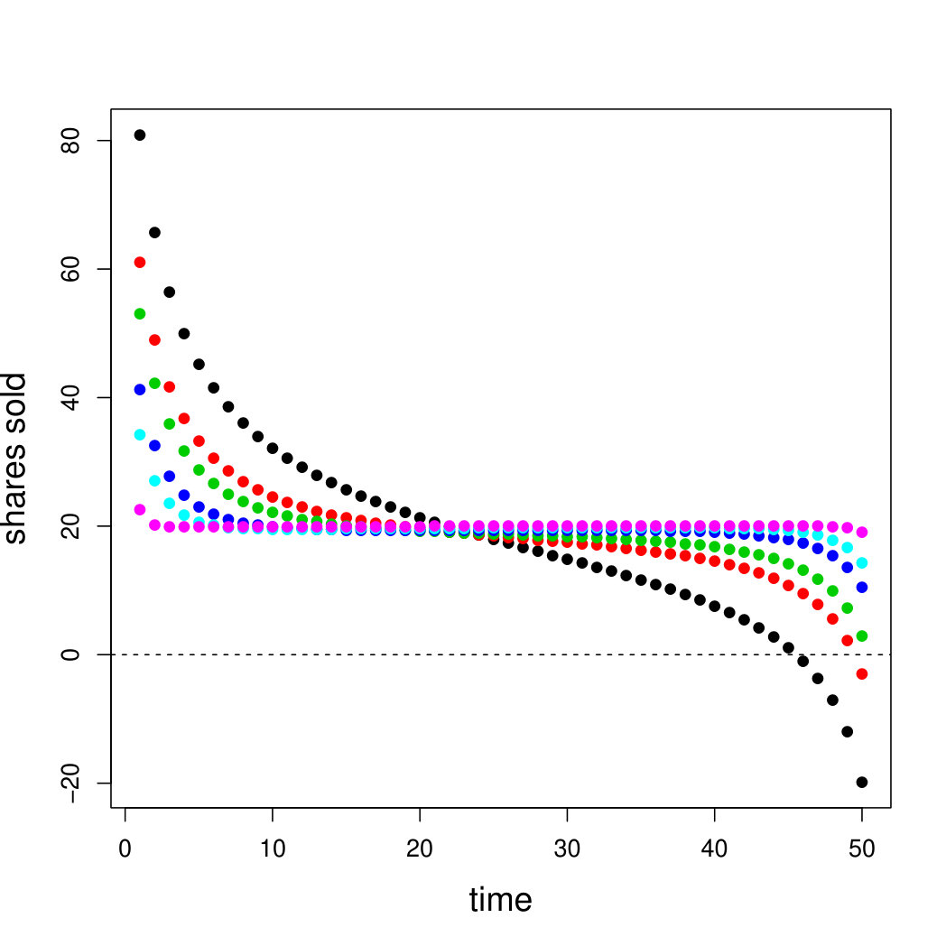 Figure 7
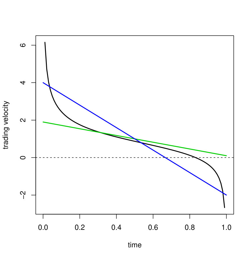 Figure 8
Peer Reviews
No public reviews on file for this paper yet. If you reviewed it on a platform where reviews are public (OpenReview, ICLR, NeurIPS, ICML), you can paste yours below so the community can read it here.
Videos
No videos yet. Explain this paper in a talk, walkthrough, or lecture? Add one.
Optimal VWAP execution under transient price impact
Alexander Barzykin and Fabrizio Lillo111Barzykin: HSBC FX eRisk, Global Markets, HSBC Bank Plc., UK. [email protected]. Lillo: Dipartimento di Matematica, Università di Bologna, Italy. [email protected]. We thank Jeanine Baumert (who participated to the early stage of this project) and James Newbury for useful discussions.
Abstract
We solve the problem of optimal liquidation with Volume-Weighted Average Price (VWAP) benchmark when the market impact is linear and transient. Our setting is indeed more general as it considers the case when the trading interval is not necessarily coincident with the benchmark interval: Implementation Shortfall and Target Close execution are shown to be particular cases of our setting. We find explicit solutions in continuous and discrete time considering risk averse investors having a CARA utility function. Finally, we show that, contrary to what is observed for Implementation Shortfall, the optimal VWAP solution contains both buy and sell trades also when the decay kernel is convex.
Keywords: Optimal execution; Volume Weighted Average Price (VWAP); Transient price impact; Transaction costs; Market microstructure.
1 Introduction
Optimal execution is becoming a hot field in market microstructure and mathematical finance. The reason is that, with the electronification and fragmentation of financial markets, the execution of a trade requires advanced infrastructure and sophisticated knowledge on how the trading orders affect prices. In a situation where the available liquidity at the best price is vanishingly small, the best strategy to minimize costs is to split the order in may trades to be executed sequentially, as postulated well before the modern markets by Kyle [19]. For this reason, starting from the seminal papers of Bertsimas and Lo [1] and Almgren and Chriss [2], many contributions have been proposed to find solve the optimal execution problem (for extensive reviews, see [14, 17, 7]).
The problem setting crucially depends on two elements: (i) the market impact model and (ii) the benchmark criterion. Concerning the first one, empirical literature [5, 22, 27, 3] has documented that the assumption of permanent and fixed market impact postulated in the original papers [1, 2] is not observed. On the contrary, market impact is transient, i.e. impact is strongest immediately after being triggered and then it decays in time, typically very slowly. This evidence has lead to the development of new models, the most famous one being the Transient Impact Model (TIM, earlier known as the propagator model) [5], whose continuous time version was proposed in [15]. Other approaches, which model in more details the limit order book [23, 12, 9] behave in some limit as the TIM model222But of course they deviate in other aspects, thus what is optimal for the TIM is not necessarily so for these other order book models.. Originally developed for modeling market impact, the TIM has immediately become subject of intense studies for the optimal execution problem. Refs. [3, 6, 10, 8] constitute an incomplete list.
All the above papers, however, solve the optimal execution problem under the assumption that the benchmark criterion is the Implementation Shortfall (IS) or Arrival Price. For a sell order, this means that the execution tries to maximize the risk adjusted difference between the expected revenue from the proceeds and the value of the order marked to market just before the execution starts. Despite being very used in academic literature, the IS is probably not the most used benchmark in the industry. More common alternatives are the Volume Weighted Average Price (VWAP)333The frequently used Time Weighted Average Price can be seen as a special case of the VWAP when the market volume is considered constant., the Target Close (TC), and the Percentage of Volume (POV). Surprisingly, relatively few studies have considered these benchmarks. Among the exceptions, Refs. [18, 20, 16, 11] considered the VWAP, but the price impact model used is the one of Almgren and Chris (with or without stochastic market volume).
To the best of our knowledge, there is no paper studying the optimal execution problem under the TIM when the execution is benchmarked against the VWAP (TWAP) or the TC. In this paper we fill this gap by solving the problem in continuous and in discrete time. We frame a setting where a broker has to sell a quantity of shares in a time window and we consider as benchmark the VWAP in an interval . In the next Section we motivate when such situation can arise in practice. Here it is worth noticing that IS, TC, and VWAP are special cases of this general problem. The first one when and , the second when and and the last one when and . Interestingly, also the case when is finite and not coincident with (dubbed interval VWAP) is of interest in practice, as detailed below.
The problem setting postulates that the broker has a CARA utility function, which is standard in this kind of problems (see, for example, [17]). We solve the problem in continuous time, by transforming the problem of maximizing of the utility function to the one of solving an integral equation, similarly to what done in [10] for the IS case. The setting of the problem in discrete time is instead useful if more constraints (for example on the maximal participation rate) must be added to the problem. In fact, the maximization of the utility function can be transformed in a quadratic optimization problem, to which additional constraints in a linear or even quadratic form can be added, without changing dramatically the complexity of the problem. Finally, the discrete case allows to add the trading volume of the execution to the benchmark, an addition that can be relevant for very large trades.
The paper is organized as follows. Section 2 introduces the TIM and its known properties also in relation to the existence of dynamic arbitrage. Section 3 sets the optimization problem in continuous time and find the equivalence with the integral equation. Moreover, explicit solution in simple cases are given. In Section 4 we restate the problem in discrete time (discussing the connections with continuous time case), solve it, and present some specific numerical examples. Finally. in Section 5 we draw conclusions and provide suggestions for further work.
2 The Transient Impact Model
Any optimal execution problem depends critically on the market impact model, i.e. on how the price reacts to trades of the execution. In this paper we will consider the Transient Impact Model (TIM) (aka the propagator model) introduced in [5] (see also [3]). Originally introduced in transaction (i.e. discrete) time, it has been generalized to continuous time in [15]. Considering a time interval and indicating with the price at time , the evolution of the price under the TIM is
[TABLE]
where is the amount of shares sold by the considered execution in , is a Wiener process in a suitable probability space, and volatility is a deterministic function. The function describes the instantaneous impact of the executed trades on price and in the linear case444Despite empirical literature suggests a nonlinear behavior of [3], models, TIM with nonlinear appears to admit price manipulation [8]. considered in this paper, it is
[TABLE]
The function , termed the kernel or propagator of the model, describes the delayed effect of trading on price and characterizes how a trade at time affects the price at time . Since is generally observed to be a decreasing function [5, 25], impact is of transient nature in this model. By contrast, other models of market impact, such as the one of Almgren and Chriss [2], postulate a permanent impact (i.e. a constant ) plus a temporary impact affecting only costs.
A significant part of the literature has considered the problem of price manipulation and dynamic arbitrage under different market impact models [15, 4, 14, 10, 8, 26]. An impact model admits price manipulation when there exists a round trip strategy leaving some profit on expectation [14]. The model, instead, admits transaction triggered price manipulation if the expected revenues of a sell (buy) program can be increased by intermediate buy (sell) trades” [4]. It is possible to show that the absence of transaction-triggered price manipulation implies the absence of price manipulation [14].
When considering the TIM as a market impact model, a series of conditions for the absence of market manipulation have been derived (see [14]). In particular, when the function in (1) is linear, the convexity of is sufficient to guarantee the absence of transaction triggered price manipulation. This result is however obtained when considering Implementation Shortfall as the function to minimize. In this paper we show that when the objective is different (in our case the VWAP), convexity of is not anymore sufficient and indeed optimal solutions for a sell program contain both buy and sell trades.
3 Problem setting in continuous time
We consider a general problem setup where a broker has to sell a quantity of shares in a time window , termed the trading interval, and she is benchmarked against the market VWAP in a time window , termed the benchmark interval. This formulation covers the majority of standard settings, such as Implementation Shortfall with , Target Close with , and interval VWAP with , . The general situation of may arise where the broker has to guarantee the VWAP price in a given time interval but is too large to be traded within this interval due to constraints (e.g., maximum POV). Point in time benchmarks, such as Market Close, provide a limiting scenario, which is typically solved with Target Close algorithm executing before Market Close. Trading after close is possible for certain instruments and may be preferable due to volatility risk reduction. Industry point in time benchmarks are being replaced with interval benchmarks, thus supporting the general formulation.
The normalization condition requires
[TABLE]
even if it is possible that , i.e. the broker can decide also to buy in the market a part of shares (if this is allowed). Let be the deterministic market volume traded in . The VWAP benchmark is given by
[TABLE]
where
[TABLE]
where is the indicator function of the set .
The objective function of the broker is the difference between the cash she is able to obtain from the proceeds in the trading interval and the cash she will give back to the client, equal to . This difference is of course a random variable, thus we must assume some utility function to model the risk aversion of the broker. To this end let us define the cash process
[TABLE]
Assuming a CARA risk averse agent, the objective function for a strategy is
[TABLE]
where is the risk aversion parameter. We can now plug in the TIM of Eq. (1) for the dynamics of price and prove the following proposition:
Proposition 1
Under linear impact, with , the maximization of the utility function (7) is equivalent to the minimization of the functional
[TABLE]
The proof of this and the following propositions are in the appendix.
In order to find the optimal execution we make use of calculus of variations following the approach of [10, 21]. We consider a strategy
[TABLE]
corresponding to a instantaneous purchase of one unit at time which is sold instantaneously at time . Indicating with the optimal strategy and setting , the integral equation satisfied by the optimal strategy is obtained by setting
[TABLE]
Although it is possible to obtain the integral equation in the general case, in the following we will restrict our attention to the case of a risk neutral investor (). In Section 4 we will explore also the case of a risk averse investor () in discrete time setting. This procedure leads to the following proposition:
Proposition 2
The strategy minimizing the functional (8) with satisfies the integral equation
[TABLE]
where is a constant set by the normalization of the total volume traded
[TABLE]
Remark 1
We remind [10] that the optimal execution under TIM when the objective function is the Implementation Shortfall satisfies the equation
[TABLE]
thus under VWAP objective function there is an additional term in the left hand side of the equation.
Remark 2
When , it is , and the second integral in Eq. 11 becomes555Note that here and in the following we use the convention that . Thus, since , when is a Dirac delta centered either at or at , we must include a factor .
[TABLE]
Since , the integral equation reduces to Eq. 13 i.e. the one obtained by Schied et al. [10] for the the optimization of the Implementation Shortfall.
We can use Remark 1 to write the solution of the integral equation as the sum of two terms. To this end we introduce the variable
[TABLE]
with and, by replacing in (11), we obtain
[TABLE]
One can write the solution where the second term solves
[TABLE]
Setting , the first term solves
[TABLE]
which is the equation when the objective function is the IS and the number of shares is .
Remark 3
When (Target Close) it is , the second integral in Eq. 11 reduces to
[TABLE]
and the integral equation becomes
[TABLE]
The solution of this integral equation is with the normalization . In other words, the optimal schedule under the TC benchmark is the sum of shares traded as in the IS case and the remaining shares traded at .
3.1 Explicit Solution for a VWAP when the benchmark interval and the trading interval coincide
We consider here the case when the benchmark VWAP interval coincides with the trading interval and , , i.e. the market volume is constant in the interval (TWAP). In this case we are able to find the explicit solution for two different kernels and compare the results with the optimal schedule obtained under different impact models. More general cases will be explored numerically using time discretization in Section 4.
3.1.1 Exponential kernel
We consider first the exponential kernel . It is known that this type of kernel is consistent with the model of Obizhaeva-Wang [23] for the resilience of the order book. We remind that when minimizing the IS, the solution is to trade a finite fraction instantaneously at times and and a fraction at constant speed in . As for any kernel, the IS optimal trading schedule is symmetric with respect to .
Defining the trading velocity , it is straightforward to test that the solution of the type
[TABLE]
satisfies (11), and, by imposing the normalization condition, we obtain the result
[TABLE]
Therefore, it is optimal to sell a finite amount at time , then selling at a constant rate for the whole interval and finally buying a finite amount at time .
Thus we see that differently from the case of IS, the optimal execution under VWAP (i) is not anymore symmetric around and (ii) allows for transaction triggered price manipulation even when is convex. As we will see next, these properties also hold for other choices of the kernel function.
3.1.2 Power law kernel
It is well known that empirical data show unambiguously that the kernel behaves as a power law for large lags [5, 3]: indeed for small tick stocks the power law behavior is observed for all values of , while for small tick stocks there is a bump for very small lags [25]. For analytical tractability we will consider here the case with .
To find the optimal solution of the VWAP execution, we use the decomposition leading to (15). We remind that in the case of IS the optimal solution for an execution of shares is [3, 10]
[TABLE]
Note that is always positive in and symmetric with respect to (U-shaped), diverging at and .
The function solves the integral equation
[TABLE]
This is a generalized Abel integral equation with constant limits [13, 24]. Using Eqs. (2.58) and (2.62) of [24], the solution can be found as666Note that the following expression can be used also for finding the optimal execution for a generic , since when the kernel is power law, Eq. 11 is a generalized Abel integral equation with constant limits.
[TABLE]
where indicates the Cauchy principal value integral. When , this expression can be rewritten as
[TABLE]
Since
[TABLE]
where is the hypergeometric function, the solution is
[TABLE]
By direct integration
[TABLE]
This value is used in the expression for and finally we obtain for the trading velocity
[TABLE]
Since , diverges positively when (as in the IS case), whereas the conditions and imply that diverges negatively for . This means that in a VWAP sell execution it is optimal to buy toward the end of the trading period and thus that this strategy allows for transaction triggered price manipulation even when is convex. Finally, it is interesting to observe that in the limit , the optimal schedule is , i.e. to trade at constant speed.
For illustrative purposes we consider the case of and . The left panel of Figure 1 shows the optimal schedule for . Clearly this solution is not symmetric w.r.t. . Moreover, qualitatively similarly to the case of exponential kernel, the optimal solution is to sell very intensely around , then to sell at a lower speed, and to buy very intensely when getting close to . When is small, the region of negative trading velocity becomes larger. On the contrary, as mentioned above, when becomes close to one, the optimal schedule becomes close to a constant with a positive and negative peak at and , respectively.
Remark 4
It is interesting to compare our solution with with the one obtained in [16] for a linear permanent impact model á la Almgren-Chriss. Assuming a linear permanent impact with constant and a quadratic temporary impact with constant , [16] finds that the optimal solution for a risk neutral agent is
[TABLE]
where and is the market volume. Figure 1 shows two solutions corresponding to (green) and (blue). Qualitatively, also in these solutions it is optimal to trade faster at the beginning of the interval and, in the case of large , (i.e. small temporary impact) it is optimal to buy back a part toward the end.
4 Solution in discrete time
In this Section we derive the solution of the optimal VWAP by using a discrete time framework. This setting will allow to obtain explicit solutions and to explore also the role of additional constraints (for example the requirement that in a sell program no buying is allowed). The discrete time setting can be applied at three different levels: (i) express the cost function (8) in discrete time and solve the optimization; (ii) use discrete time to obtain a quadrature of the integral equation (15); (iii) write the TIM (1) in discrete time, derive the corresponding cost, and then minimize it. It is worth noticing that the three procedures do not give exactly the same result, however if the time intervals used in the discretization are sufficiently small, the differences become negligible. In the following we will consider approach (iii) and we will briefly discuss the difference with approach (i).
Let us divide the interval in equal intervals and define . The strategy is now a vector , where is the amount of shares traded in interval , i.e. for . The price dynamics of a sell execution in discrete time is
[TABLE]
which can be rewritten in vector form as
[TABLE]
where , , is the lower triangular matrix of ones (i.e. if , zero otherwise), and is the lower triangular matrix such that if and zero otherwise. Finally is a Gaussian random vector describing the price dynamics without execution. Even if in the following we will focus mainly on and , we will provide solutions in the presence of drift and correlated returns. The cash amount at the end of the period is .
In full generality, we consider a VWAP benchmark between and , corresponding to are the rounding to the nearest integer giving the initial and final trading intervals. We indicate and we introduce a vector with components
[TABLE]
where is the market volume traded in interval and is the indicator function777For the moment we are neglecting our trading on the benchmark, see the subsection 4.2.. The benchmark is and the normalization ensures that . The utility function is and, using the Gaussian assumption under CARA utility function with risk aversion , the expected utility is
[TABLE]
In the Appendix we prove the following proposition.
Proposition 3
Under CARA utility function with risk aversion , the optimal VWAP execution, which maximizes the expected utility (28), is the solution of the quadratic optimization
[TABLE]
where
[TABLE]
Moreover, the matrix is positive definite if is positive definite. Thus the solution of the quadratic optimization exists and is unique.
Since the problem can be recast in a quadratic optimization form, several additional constraints can be added without affecting the difficulty of the problem. For example, it is possible to add the constraint that all the trades have the same sign, e.g. no buys in a sell execution (), or a constraint on the maximal trading speed ().
Remark 5
Note that when and , one does not obtain the same solution derived by discretizing the cost function. This is because here we have discretized the impact model and not the cost. The difference between the two solutions is due to the diagonal terms of which when discretizing the cost are half than those obtained by discretizing the impact model. The difference between the strategies is however small and tends to zero when .
4.1 Numerical results
In this section we explore the optimal solutions under different parameter choices. In all analyses we will set , , , and . Moreover we choose a power law kernel with . Finally we assume a flat market volume profile, i.e. .
Figure 2 shows the baseline case where (i.e. a risk neutral broker), (no drift), and . The red dots refer to the unconstrained problem, while the blue ones to the case with constraint . The first one is similar to the solution in continuous time shown in Fig. 1 with negative positions (buys) toward the end of the execution, while in the second one the negative are essentially capped to zero. In both cases the value of the expected utility, which in the risk neutral case corresponds to the expected cash minus the VWAP, is positive indicating a liquidation value larger than the VWAP, thus a net profit for the broker.
We then consider the role of drift and risk aversion. Left panel of Fig. 3 shows the optimal solution for risk neutral agents and different values of the (constant) drift. Blue (red) lines refer to positive (negative) drift, while the black line refers to the driftless benchmark case. As is intuitive, when the drift is positive (negative), it is optimal to delay (anticipate) the sale of the shares. The right panel of Fig. 3 shows the optimal solution in the driftless case for different risk aversion parameter . We set with a constant volatility .
Remark 6
It is interesting to note that for very large risk aversion, the optimal trading profile becomes flat, i.e. if the broker cares only about the variance of the profit, the optimal choice is to trade at constant speed, which, under the assumption of constant market volume , means fixed percentage of volume (like in a POV strategy). Note that this is different to what happens under IS benchmark [6], since in this case the risk neutral U-shape becomes asymmetric and the strategy is front loaded (i.e. more trading at the beginning of the execution than at the end)
We now come to the case of the benchmark period not coincident with the trading period . Figure 4 shows the solution for drifless prices and risk neutral broker when and . The figure shows the result with (black) and without (red) constraint on the sign of the trades. We observe that the optimal solution is to trade before, during, and after the benchmark interval. If the constraint that all the trades must have the same sign is imposed, it is optimal not to trade after the benchmark period. Interestingly, before the start of the benchmark period the trading pattern resembles the U-shape of the optimal execution under IS (see Eq. 18 for the expression in continuous time), while during the benchmark period the trading pattern is similar to the one obtained when the trading interval coincides with the benchmark interval (see Fig. 2).
Finally, we consider how the expected excess profit of the broker depends on the benchmark interval. The excess profit is the difference between the cash at the end of the trading period and the VWAP in the benchmark period (which is the cash given by the broker to the client). We again consider , drifless prices, risk neutral broker, and the other parameters as above. The left panel of figure 5 shows the expected excess profit of a benchmark period centered in and of variable length. It is clear that the interval providing the largest profit is the shortest one. Given this result, the right panel shows the excess profit for a benchmark period of length one as a function of the time within the trading period where the benchmark period is located. The shape is non-monotonic and, for the chosen parameter, the benchmark period providing the largest profit is of length one and located at time .
In conclusion the benchmark period providing the largest profit is very short and located in the second half of the trading interval. It is important to remark however that we have implicitly assumed that the market impact model of Eq. (1) continues to hold also for the very large trading intensities required for short benchmark periods. This is unlikely in reality and additional constraints (for example on the maximal trading speed) should be added to the optimization of Proposition 3 to have more realistic results.
4.2 Including executed volume in the benchmark
Especially for short benchmarks, the volume coming from the optimal execution can be a significant fraction of the market volume and therefore one should add it to build the benchmark. Thus Eq. (27) can be imprecise and should be replaced by
[TABLE]
Due to the fact that appears with absolute value and in the denominator, plugging this benchmark price in the optimization leads to a non quadratic optimization which can be very hard to solve. We will consider here the case when , leading to the expansion
[TABLE]
Note that the norm of this vector, , is equal to one. For simplicity we consider the case and denote with the length of the benchmark time, thus
[TABLE]
The argument of the utility function can be rewritten as where and
[TABLE]
and is the identity matrix and is the unit matrix (matrix where all elements are ones). In conclusion the optimization is the same as before with the only change
5 Conclusions
In this paper we have set and solved the problem of the optimal execution of an order when the benchmark is the volume weighed average price on a specific time interval and the price impact is transient. By considering the general case when the trading interval is larger than the benchmark interval, we have shown that several existing optimal execution benchmarks (Implementation Shortfall, Target Close, VWAP, and TWAP) can be seen as special cases. We have considered the solution in continuous time, mapping the maximization problem into the solution of an integral equation, in line with what was done for IS in [10]. Solution in discrete time has been reduced to standard quadratic optimisation problem. We have not explicitly considered transaction costs and child order placement as being part of optimisation which would be required for practical applications. One of the ways to approximately take this into account is by incorporating tactical cost into the impact kernel [6]
Appendix A Proofs of propositions
A.1 Proof of proposition 1
Since is a Gaussian distributed variable, the broker maximizes
[TABLE]
The expected value is
[TABLE]
because the first term identically vanishes due to the normalization of and and the third term is the expectation of a stochastic integral.
In the case of linear impact, this becomes
[TABLE]
Similarly for the variance term
[TABLE]
The last expectation can be written as
[TABLE]
Finally, given that and , the maximization of the utility is equivalent to the minimization of the functional of Eq. (8).
A.2 Proof of proposition 2
The quantity to minimize in a VWAP execution is
[TABLE]
that we rewrite as .
Following [10, 21], we consider a strategy
[TABLE]
and indicate with the optimal strategy. Hence, setting , it is
[TABLE]
where . The quantity
[TABLE]
where is the step function, while
[TABLE]
If the strategy is optimal then
[TABLE]
i.e. if
[TABLE]
or equivalently
[TABLE]
where is a constant set by the normalization on the total volume traded
[TABLE]
Generically we will be interested in the trading velocity defined in , thus we solve
[TABLE]
A.3 Proof of proposition 3
The utility function is . Since everything is Gaussian and assuming as in the continuous time case a CARA utility function with risk aversion , the expected utility is
[TABLE]
The mean value term is
[TABLE]
where the first term vanishes because and .
The variance term is
[TABLE]
[TABLE]
Thus the maximization of the expected utility is equivalent to the minimization of
[TABLE]
which can me rewritten in matrix form as
[TABLE]
where and are given in Eq. (29) and (30) and
[TABLE]
is a constant not affecting the optimal solution (but of course affecting the value of the optimal expected utility).
To prove that is Positive Definite (PD), let us note first that is PD, since it is lower triangular with diagonal elements . The other term, can be rewritten as , where and is the lower triangular matrix obtained from the Cholesky decomposition of (which exists because is PD). Clearly is lower triangular with the same diagonal entries of . These entries are positive, again because is PD, and therefore is invertible. The product of an invertible matrix and its transpose, such as , is PD. Finally, is the sum of two PD matrices, and therefore it is PD.
The reference list from the paper itself. Each links out to its DOI / PubMed record.
- 1[1] Bertsimas, D. & Lo, A. (1998), Optimal Control of Execution Costs, Journal of Financial Markets 1 1–50.
- 2[2] Almgren, R., & Chriss, N. (2000), Optimal Execution of Portfolio Transactions, J. Risk 3 5–39.
- 3[3] Bouchaud, J.-P., Farmer, J.D. & Lillo, F. (2009), How markets slowly digest changes in supply and demand. In Handbook of Financial Markets: Dynamics and Evolution , edited by T.Hens and K. Schenk-Hoppe, Academic Press: New York.
- 4[4] Alfonsi, A., Schied, A., & Slynko, A. (2012), Order book resilience, price manipulation, and the positive portfolio problem. SIAM Journal on Financial Mathematics , 3 (1), 511-533.
- 5[5] Bouchaud, J.-P., Gefen, Y., Potters, M. & Wyart, M. (2004), Fluctuations and response in financial markets: the subtle nature of ’random’ price changes, Quantitative Finance 4 176–190.
- 6[6] Busseti, E. & Lillo, F. (2012), Calibration of optimal execution of financial transactions in the presence of transient market impact, J. Stat. Mech. P 09010.
- 7[7] Cartea, A., Jaimungal, S., & Penalva, J. (2015). Algorithmic and High-Frequency Trading . Cambridge University Press.
- 8[8] Curato, G., J. Gatheral, & F. Lillo (2017), Optimal execution with nonlinear transient market impact, Quantitative Finance 17 , 41-54