Travelling Corners for Spatially Discrete Reaction-Diffusion System
Hermen Jan Hupkes, Leonardo Morelli

TL;DR
This paper demonstrates the existence of travelling corner solutions in spatially discrete reaction-diffusion systems, extending planar travelling waves into corner solutions using a novel reduction technique.
Contribution
It introduces a new method to continue stable planar travelling waves into corner solutions in lattice reaction-diffusion equations, especially when the group velocity is zero.
Findings
Corners exist in Nagumo lattice systems with stable planar waves.
A non-standard center manifold reduction is used to analyze bifurcations.
The approach handles regularity issues caused by spatial discreteness.
Abstract
We consider reaction-diffusion equations on the planar square lattice that admit spectrally stable planar travelling wave solutions. We show that these solutions can be continued into a branch of travelling corners. As an example, we consider the monochromatic and bichromatic Nagumo lattice differential equation and show that both systems exhibit interior and exterior corners. Our result is valid in the setting where the group velocity is zero. In this case, the equations for the corner can be written as a difference equation posed on an appropriate Hilbert space. Using a non-standard global center manifold reduction, we recover a two-component difference equation that describes the behaviour of solutions that bifurcate off the planar travelling wave. The main technical complication is the lack of regularity caused by the spatial discreteness, which prevents the symmetry group from…
Click any figure to enlarge with its caption.
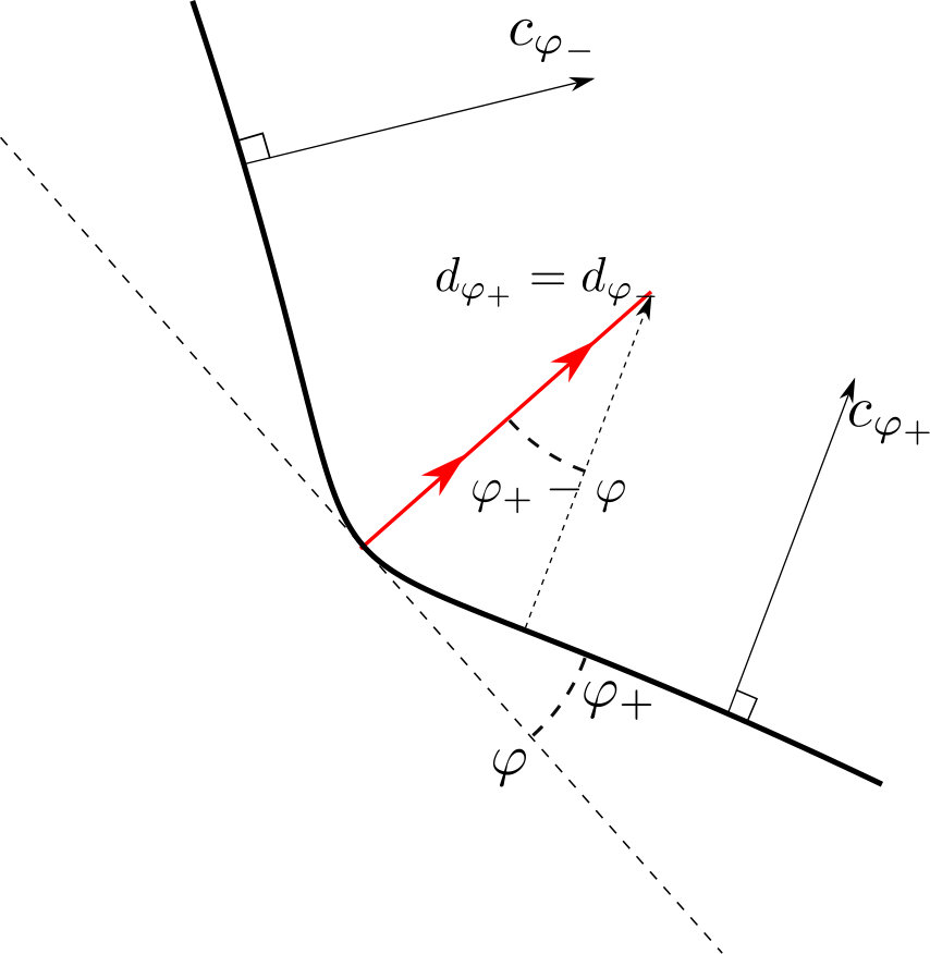 Figure 1
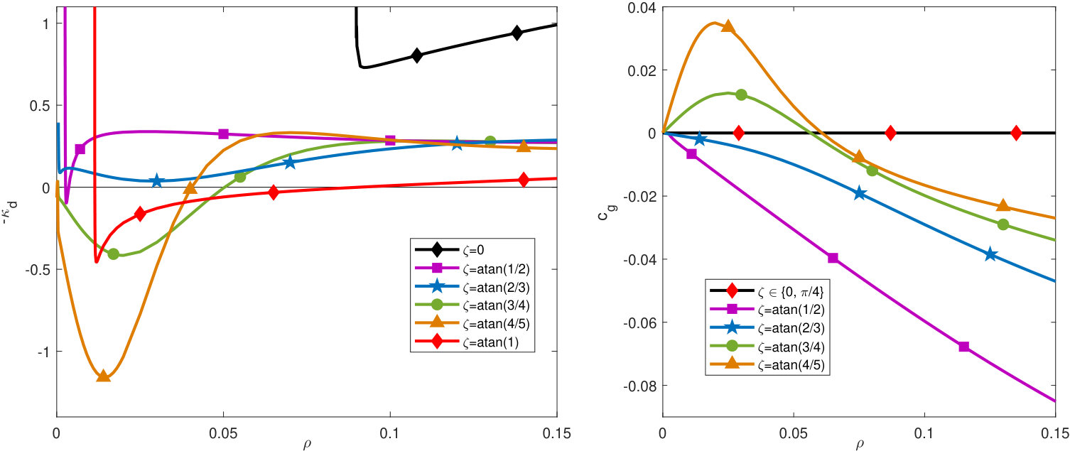 Figure 2
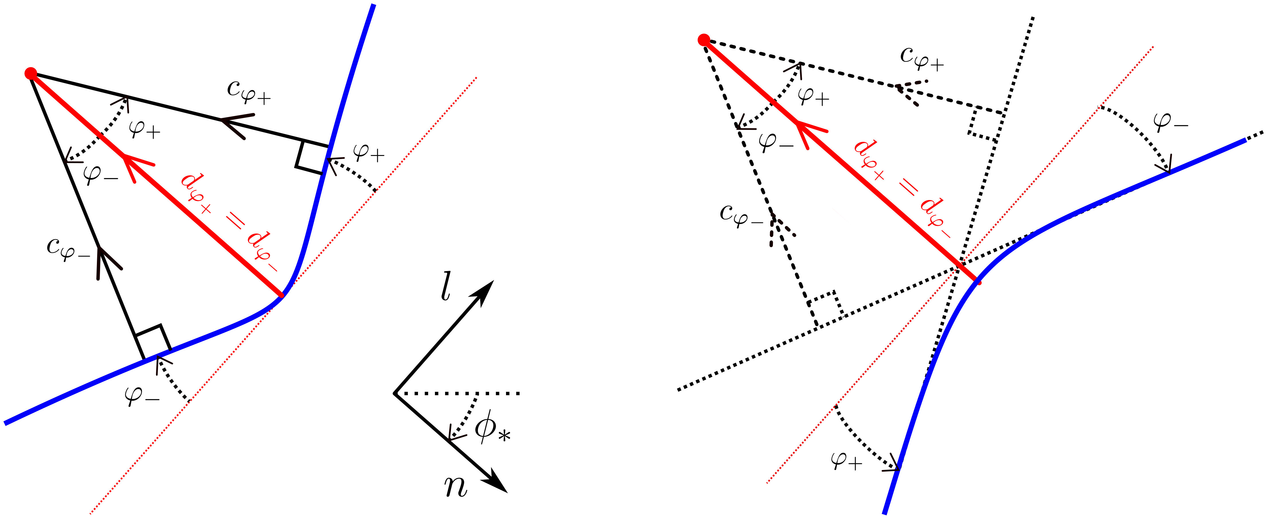 Figure 3
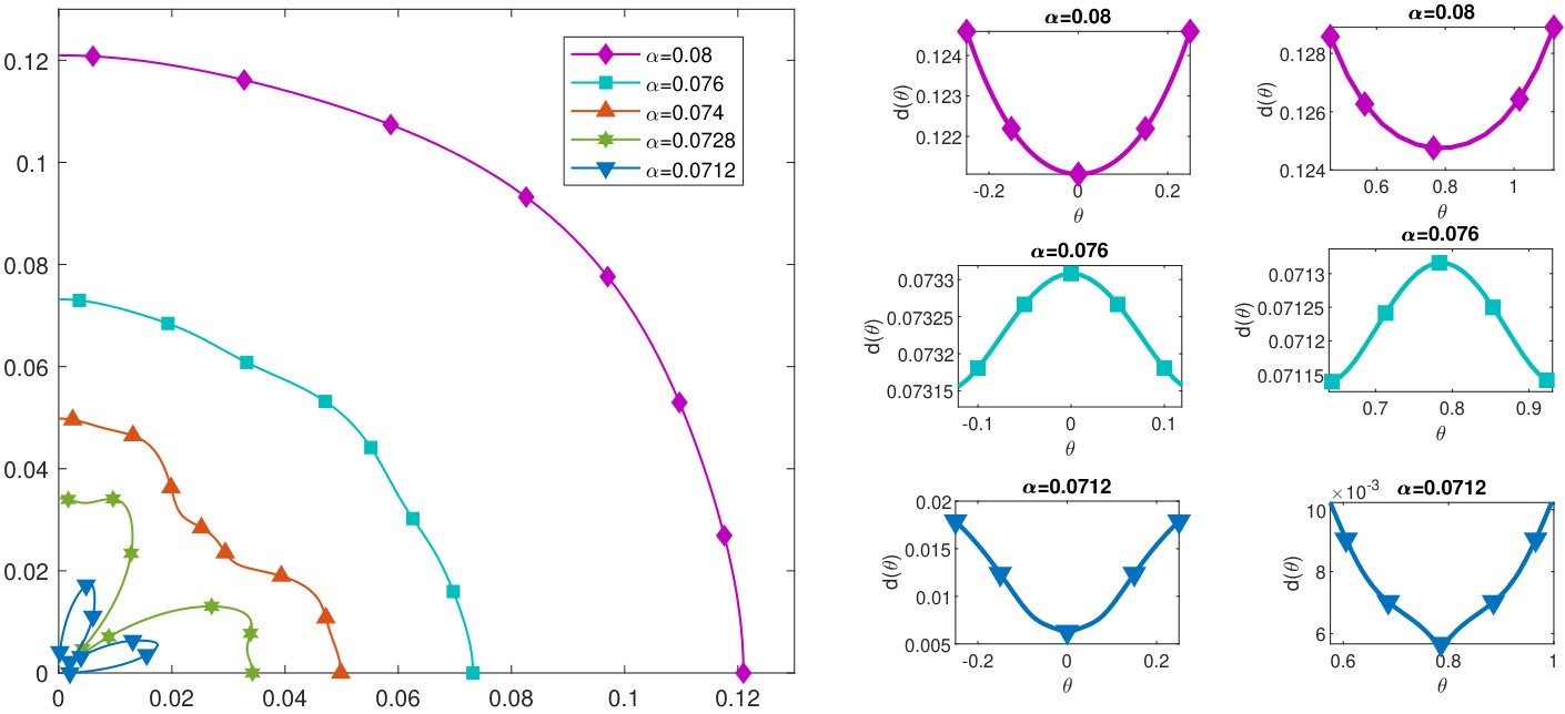 Figure 4
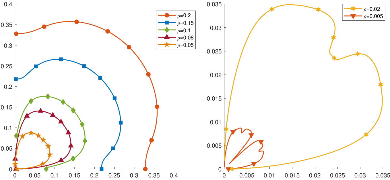 Figure 5
Peer Reviews
No public reviews on file for this paper yet. If you reviewed it on a platform where reviews are public (OpenReview, ICLR, NeurIPS, ICML), you can paste yours below so the community can read it here.
Videos
No videos yet. Explain this paper in a talk, walkthrough, or lecture? Add one.
Taxonomy
TopicsNonlinear Dynamics and Pattern Formation · Mathematical and Theoretical Epidemiology and Ecology Models · Stability and Controllability of Differential Equations
Travelling Corners for Spatially Discrete
Reaction-Diffusion Systems
H. J. Hupkes
L. Morelli \corauthrefcoraut
(Version of )
Abstract
We consider reaction-diffusion equations on the planar square lattice that admit spectrally stable planar travelling wave solutions. We show that these solutions can be continued into a branch of travelling corners. As an example, we consider the monochromatic and bichromatic Nagumo lattice differential equation and show that both systems exhibit interior and exterior corners.
Our result is valid in the setting where the group velocity is zero. In this case, the equations for the corner can be written as a difference equation posed on an appropriate Hilbert space. Using a non-standard global center manifold reduction, we recover a two-component difference equation that describes the behaviour of solutions that bifurcate off the planar travelling wave. The main technical complication is the lack of regularity caused by the spatial discreteness, which prevents the symmetry group from being factored out in a standard fashion.
{frontmatter}\journal
…
,
\corauth[coraut]Corresponding author.
\address
[LD1] Mathematisch Instituut - Universiteit Leiden
P.O. Box 9512; 2300 RA Leiden; The Netherlands
Email: [email protected]
\address[LD2] Mathematisch Instituut - Universiteit Leiden
P.O. Box 9512; 2300 RA Leiden; The Netherlands
Email: [email protected]
{subjclass}
34A33 \sep35B36.
{keyword}
travelling corners, anisotropy, lattice differential equations, global center manifolds.
1 Introduction
In this paper we construct travelling corner solutions to a class of planar lattice differential equations (LDEs) that includes the Nagumo LDE
[TABLE]
posed on the two-dimensional square lattice , in which the nonlinearity is given by the bistable cubic
[TABLE]
Such corners can be seen as interfaces that connect planar waves travelling in slightly different directions. In particular, our analysis does not require the use of the comparison principle, but merely requires a number of spectral and geometric conditions to hold for the underlying planar travelling waves. This allows our results to be applied to a wide range of LDEs, highlighting the important role that anisotropy and topology play in spatially discrete settings.
Reaction-diffusion systems
The LDE (1.1) can be seen as a nearest-neighbour spatial discretization of the Nagumo PDE
[TABLE]
In modelling contexts one often uses the two stable equilibria of the nonlinearity to represent material phases or biological species that compete for dominance in a spatial domain. Indeed, the diffusion term tends to attenuate high frequency oscillations, while the bistable nonlinearity promotes these. The balance between these two dynamical features leads to interesting pattern forming behaviour.
As a consequence, the PDE (1.3) has served as a prototype system for the understanding of many basic concepts at the heart of dynamical systems theory, including the existence and stability of planar travelling waves, the expansion of localized structures and the study of obstacles. Multi-component versions of (1.3) such as the Gray-Scott model [19] play an important role in the formation of patterns, generating spatially periodic structures from equilibria that destabilize through Turing bifurcations. Memory devices have been designed using FitzHugh-Nagumo-type systems with two components [31], which support stable stationary radially symmetric spot patterns. Similarly, one can find stable travelling spots [46] for three-component FitzHugh-Nagumo systems, which have been used to describe gas discharges [38, 42].
At present, a major effort is underway to understand the impact that non-local effects can have on reaction-diffusion systems. For example, many neural field models include infinite-range convolution terms to describe the dynamics of large networks of neurons [10, 11, 39, 43], which interact with each other over long distances. The description of phase transitions in Ising models [3, 4] features non-local interactions that can be both attractive and repulsive depending on the length scale involved.
It is well-known by now that the topology of the underlying spatial domain can have a major impact on the dynamical behaviour exhibited by such non-local systems. For example, nerve fibers have a myeline coating that admits gaps at regular intervals [40], which can block signals from propagating through the fiber [15, 30, 34]. In order to study the growth of plants, one must take into account that cells divide and grow in a fashion that is influenced heavily by the spatial configuration of their neighbours [20]. Finally, the periodic structure inherent in many meta-materials strongly influences the phase transitions that can occur [13, 14, 44] as a consequence of the visco-elastic interactions between their building blocks.
We view the planar LDE (1.1) as a prototype model that allows the impact of such non-local spatially-discrete effects to be explored. Indeed, the spatial transition breaks the locality but also the translational and rotational symmetry of (1.3), leading to several interesting phenomena and mathematical challenges.
Existence of planar waves
It is well-known that the balance between the diffusion and reaction terms in the PDE (1.3) is resolved through the formation of planar travelling wave solutions
[TABLE]
which connect the two stable equilibria . When , these waves can be thought of as a mechanism by which the fitter species or more energetically favourable phase invades the spatial domain. The existence of these waves can be obtained by applying a phase-plane analysis [18] to the travelling wave ODE
[TABLE]
which results after substituting (1.4) into (1.3).
On the other hand, substitution of the analogous Ansatz
[TABLE]
into the LDE (1.1) leads to the mixed-type functional differential equation (MFDE)
[TABLE]
The broken rotational invariance in the transition from (1.3) to (1.1) is manifested by the explicit presence of the propagation direction in (1.7). The broken translational invariance causes the wavespeed to appear in (1.7) as a singular parameter.
A comprehensive existence theory for solutions to (1.7) was obtained in [36]. In particular, for every and there exists a unique wavespeed for which (1.7) admits a solution. However, it is a delicate question to decide whether or . Indeed, a sufficient energy difference between the two stable equilibrium states is needed for the propagation of waves [4, 6, 17, 33], a phenomenon referred to as propagation failure. In fact, due to the angular dependence in (1.7), planar waves can fail to propagate in certain directions that resonate with the lattice, whilst travelling freely in others [12, 25, 37].
Linearization
It is well-known that planar travelling waves can be used as a skeleton to describe the global dynamics of the PDE (1.4) [1]. In particular, they have been used as building blocks to construct other more complicated types of solutions. A key ingredient in such constructions is to understand the dynamics of the system that arises after linearizing (1.3) around the planar waves (1.4).
Performing this linearization for , we obtain the system
[TABLE]
which can be transformed to the temporally autonomous system
[TABLE]
by the variable transformation . Since this system is also autonomous with respect to the -coordinate, which is transverse to the motion of the wave, it is convenient to apply a Fourier transform in this direction. Upon introducing the symbol
[TABLE]
we readily find
[TABLE]
Inspecting (1.10), we readily see that the spectrum of can be obtained by rigidly shifting the spectrum of by . In particular, writing , we find that
[TABLE]
Noting that , we hence see that perturbations of the form evolve under (1.9) according to the heat semiflow . These perturbations are important because they correspond at the linear level with transverse deformations of the planar wave interface.
On the other hand, linearizing the LDE (1.1) around the spatially-discrete wave (1.6) that travels in the horizontal direction , we obtain the temporally non-autonomous system
[TABLE]
Although the time dependence cannot be readily transformed away, it is still possible to take a discrete Fourier transform in the -direction. This leads to the system
[TABLE]
Looking for solutions of the form
[TABLE]
we arrive the eigenvalue problem
[TABLE]
for the linear operator
[TABLE]
The theory developed in [5, 7] essentially justifies this formal calculation and confirms that the spectral properties of can be used to understand the dynamics of the time-dependent problem (1.14). Upon writing , we again have
[TABLE]
To find the evolution of perturbations of the form under (1.14), we must now solve the discrete heat equation
[TABLE]
The situation is hence similar to that encountered for the PDE (1.3).
More material changes arise however when considering the diagonal direction . Following a similar procedure as above, one arrives at the linear operator
[TABLE]
which has a spectrum that can no longer be directly related to that of . It is hence no longer clear how to formulate an analogue for (1.19) to describe the linear evolution of interface deformations. However, it is still the case that as for the curve of eigenvalues that bifurcates from the zero eigenvalue .
For general rational angles this quadratic behaviour need no longer be true. In fact, we obtain the relation
[TABLE]
for the quantity that is often referred to as the group velocity. A similar relation was found in [21] for planar PDEs with direction-dependent diffusion coefficients. However, in this case it is always possible to change the coordinate system in such a way that holds again.
Such a transformation is not possible in the spatially discrete setting (1.1), since this would require the transverse spatial coordinate to become continuous. However, we do remark here that the function can behave rather wildly in the critical regime where is small, allowing the group velocity to vanish at specific values for even if .
Stability of planar waves
The realization that transverse interfacial deformations are governed by a heat equation led to the development of two main approaches to establish the nonlinear stability of the planar waves (1.4). Both approaches exploit the coordinate system
[TABLE]
in the neighbourhood of the planar travelling wave and require the initial perturbations and to be localized in a suitable sense.
The first approach was pioneered by Kapitula in [32], where he used semigroup methods and fixed-point arguments to show that tends algebraically to zero, while decays exponentially fast. The advantage of this approach is that only weak spectral assumptions need to be imposed on the underlying system. However, the crude estimates on the nonlinear terms lead to rather weak estimates for the basin of attraction.
The second approach leverages the comparison principle to obtain stability for a much larger class of initial perturbations. By slowing down the natural decay-rate of the fundamental solution of the heat equation, the authors of the landmark paper [8] were able to construct explicit super and sub-solutions to (1.3) that trap perturbations that can be arbitrarily large (but localized). In fact, the authors use their construction to show that these planar waves can pass around large compact obstacles and still eventually recover their shape.
In [23, 24] these approaches were generalized to the discrete setting of (1.1), thereby continuing the early work by Bates and Chen [2] featuring a related four-dimensional non-local problem. In both cases the key technical challenge was the analysis of troublesome non-selfadjoint terms spawned by the anisotropy of the lattice, especially in situation where the group velocity does not vanish. These terms have slower decay rates than their PDE counterparts and hence require special care to close the nonlinear bootstrapping procedure. For example, the sub-solutions in [8] consist of only two terms, while 33 terms were required in [23] to correct for the slower decay.
Spreading phenomena
The classic result [1, Thm. 5.3] obtained by Weinberger for the PDE (1.3) states that large compact blobs with inside and outside can expand throughout the plane. The proof of this result relies on the construction of radially expanding sub- and super-solutions by glueing together planar travelling waves.
In [23] a weak version of this expansion result was established for the LDE (1.1) in the special case that no direction is pinned. However, the underlying sub- and super-solutions expand at the speeds and respectively, which still leaves a considerable hole in our knowledge of the expansion process. Indeed, the numerical results in [45] provide strong evidence that the limiting shape of the expanding blob can be found by applying the Wulff construction [41] to the polar plot of the relation. For a large subset of parameters this limiting shape resembles a polygon.
The main motivation behind the current paper is to take a step towards understanding this expansion process by looking at the evolution of a single corner. Indeed, when the expanding blob is sufficiently large, it would seem to be very reasonable to assume that the corners of the polygon behave in an almost independent fashion.
Corners for PDEs
Assuming for concreteness that , the horizontal planar wave given by (1.4) with satisfies , which means that it travels towards the left. In [22] Haragus and Scheel construct travelling corner solutions to (1.3) by ‘bending’ this planar wave to the left in the spatial limits , so that the interface resembles a sign.
In particular, for any small opening angle , the authors establish the existence and stability of solutions of the form
[TABLE]
Here uniformly in , while the phase satisfies the limits
[TABLE]
Notice that the horizontal speed of these corners is faster than the original speed of the planar wave.
The result is obtained by using the change of variable to recast (1.3) as
[TABLE]
and subsequently demanding . The resulting system can be written in the first-order form
[TABLE]
which admits the family of -independent equilibria
[TABLE]
The linearization of (1.26) around can be written as
[TABLE]
This system admits the -independent solutions caused by the translational invariance, together with the linearly growing solution . In particular, the desired corner (1.23) lives on the two-dimensional global center manifold associated to the family (1.27). The solutions on this manifold can be represented in the form
[TABLE]
for some function
[TABLE]
One can subsequently obtain two skew-coupled ODEs to describe the dynamics of the scalar functions and . A relatively straightforward analysis shows that these ODEs have solutions for which satisfies the limits (1.24), while remains small. This suffices to establish the existence of the corners (1.23).
In addition, in [21] anisotropic effects were introduced into the problem by allowing the nonlinearity to depend on the gradient of and considering non-diagonal diffusion coefficients. In such cases the group velocity defined by the quantities (1.21) need not vanish, but it can be removed by applying a coordinate transformation in the transverse direction.
By restricting their attention to small opening angles and using center manifold arguments, Scheel and Haragus were also able to apply their techniques to multi-component reaction-diffusion PDEs such as the FitzHugh-Nagumo and Gray-Scott equations [21, 22] However, it is also possible to consider large opening angles when considering equations that admit a comparison principle. Indeed, in [9] explicit sub- and super-solutions are used to construct corners for the Nagumo PDE (1.3) that can be arbitrarily sharp.
Corners for LDEs
The crucial point in the analysis outlined above for the corners (1.23) is that the phase shift can be completely factored out from the system. This implies that the ODE for does not depend on . In addition, it allows the center manifold to be constructed by a standard fixed point argument analogous to the local case.
This is possible because the right-hand side of (1.28) maps into , which roughly means that its inverse gains an order of regularity in both components. This precisely compensates for the loss of regularity that arises by factoring out the phase-shift.
However, when attempting to mimic this procedure for the LDE (1.1) one runs into a fundamental difficulty. Indeed, the analog of (1.28) has a right-hand side that now maps into due to the lack of second derivatives in the equation. This forces us to construct a full two-dimensional global center manifold that takes into the account the dynamics of and simultaneously.
A similar situation was encountered by one of the authors in [27], where modulated travelling wave solutions were constructed to a class of non-local systems. However, the analog of (1.28) is a difference equation rather than a differential equation. The order of this difference equation can become arbitrarily large depending on the height of the fraction , which we require to be rational. Nevertheless, the final step in our analysis requires us to uncover a first-order difference equation for the center variables.
The main technical contribution in this paper is that we adapt the spirit of the approach in [27] to construct global center manifolds for the differential-difference systems that we encounter here. This approach uses two intertwined fixed point procedures to separate the flow problem for the two center variables from the task of capturing the shape of the remainder function . The underlying linear problems have non-autonomous slowly-varying coefficients, for which we develop appropriate solution operators.
In this paper we do require the group velocity (1.21) to vanish. Unlike in the spatially continuous setting, this cannot always be arranged by a simple variable transformation. Indeed, such a transformation would force the spatial variable transverse to the propagation direction to become continuous, destroying the difference structure of the system. This prevents us from exploiting the periodicity in the Fourier variable. As a result, resonances start to appear in the spectrum that are very hard to control. A similar situation was encountered in [27], which forced the authors to add a smoothening term to the underlying system.
We emphasize that the group velocity for (1.1) vanishes automatically in the directions and . In addition, directions where the wavespeed is minimal (and hence the group velocity is zero) play an important role in the Wulff construction, which is the primary motivation for our analysis here. In any case, the delicate behaviour of the map for the Nagumo LDE (1.1) leads to a much richer class of behaviour than that displayed by its continuous counterpart (1.3). For example, the latter only features interior corners, while the former can also admit exterior corners. The former also allows for so-called bichromatic corners, which connect spatially homogeneous equilibria to checkerboard patterns.
While we are confident that our center manifold construction will also allow us to establish the (linearized) stability of the corners constructed here along the lines of the approach in [21], we do not pursue this in the present paper. The main reason is that there is no coordinate transformation that can freeze our corners and also leave the discrete structure of the equation intact. One would need to generalize the approach developed in [7, 5, 24] to accommodate solutions that vary in two directions instead of just one, which we expect to be a tedious task.
Organization
Our main results are formulated in §2 and applied to the Nagumo LDE (1.1) in §2.1-2.2. In §3 we derive the differential-difference system that the pair must satisfy and formulate the global center manifold result. We proceed in §4 by deriving a representation formula for solutions to the linearized problem with constant phase. This requires us to compute a convoluted spectral projection operator that arises from the second order pole that the operator has in . In §5-§6 we combine this representation formula with Fourier analysis to construct a solution operator for the linearized problem where the phase is allowed to vary slowly. Finally, we setup the fixed point problems required to build the global center manifold in §7, appealing at times to the results in [27] for overlapping parts of the program.
Acknowledgements
HJH acknowledges support from the Netherlands Organization for Scientific Research (NWO) (grant 639.032.612). LM acknowledges support from the Netherlands Organization for Scientific Research (NWO) (grant 613.001.304).
2 Main Results
In this paper we consider the nearest-neighbour lattice differential equation
[TABLE]
posed on the planar lattice , in which takes values in . For convenience, we introduce the operator that acts as
[TABLE]
for any , which allows us to rewrite (2.1) in the condensed form
[TABLE]
The plus sign corresponds with the fact that a ”+”-shaped stencil is used to sample .
The conditions we impose on the nonlinearity are summarized in the following assumption.
- (Hf)
The nonlinearity is -smooth for some and there exist two points with
[TABLE]
We emphasize that the two points are allowed to be equal. These two equilibria are required to be connected by a planar travelling wave solution to (2.1). In particular, we pick an arbitrary rational direction with and impose the following condition.
- (H)
There exists a wave speed and a wave profile so that the function
[TABLE]
satisfies (2.1) for all . In addition, we have the limits
[TABLE]
Upon introducing the operator that acts as
[TABLE]
we note that the pair must satisfy the functional differential equation of mixed type (MFDE)
[TABLE]
In particular, the -continuity mentioned in (H) is automatic upon assuming that is merely continuous.
For convenience, we now introduce the new coordinates
[TABLE]
which are parallel respectively orthogonal to the direction of motion of the wave (2.5). Upon introducing the notation
[TABLE]
the LDE (2.3) transforms into the equivalent problem
[TABLE]
which admits the travelling wave solution
[TABLE]
A standard approach towards establishing the stability of the wave (2.12) under the nonlinear dynamics of the LDE (2.11) is to consider the linear variational problem
[TABLE]
Looking for a solution of the form
[TABLE]
we readily find that must satisfy the eigenvalue problem
[TABLE]
Here the linear operator acts as
[TABLE]
with shifts and functions that are given by
[TABLE]
Since approaches as , it is possible to define the characteristic -valued functions
[TABLE]
Our first spectral assumption states that these characteristic functions cannot have roots on the imaginary axis whenever is purely imaginary.
For all and we have
[TABLE]
We note that (2.19) can be used to rule out kernel elements of that behave as as . In fact, using [35, Thm. A] we see that (HS1) implies that is a Fredholm operator for all . Our next condition demands that these operators are actually invertible for .
For any the operator is invertible as a map from into .
Since the Fredholm index varies continuously, (HS1) and (HS2) together imply that the Fredholm index of is zero. The translational invariance of the problem implies that , which means that zero is an eigenvalue for . Our next assumption states that this eigenvalue is in fact algebraically simple.
We have the characterization
[TABLE]
and the algebraic simplicity condition
[TABLE]
For any we now introduce the linear operator
[TABLE]
that acts as
[TABLE]
An easy computation shows that
[TABLE]
holds for all pairs . For these reason, we refer to this operator as the formal adjoint of .
Using [35, Thm. A] together with , one sees that the kernel of must also be one-dimensional. In particular, it is spanned by a function that can be uniquely fixed by the identity
[TABLE]
on account of (2.21). We note that (HS1) implies that both and decay exponentially as .
We now explore two important consequences of the algebraic simplicity condition (HS3). The first of these states that the zero eigenvalue can be extended to a branch of eigenvalues for when is small.
Lemma 2.1** (see [24, Prop. 2.2]).**
Assume that (Hf), and (HS1)-(HS3) are all satisfied. Then there exists a constant together with pairs
[TABLE]
defined for each with , such that the following hold true.
- (i)
The characterization
[TABLE]
together with the algebraic simplicity condition
[TABLE]
hold for each with .
- (ii)
We have , and the maps and are analytic.
- (iii)
The normalization condition
[TABLE]
holds for every with .
The second consequence is that wave travelling in the rational direction can be perturbed to yield waves travelling in nearby directions. In particular, we introduce the constants by writing
[TABLE]
Looking for solutions to the LDE (2.11) of the form
[TABLE]
a short computation shows that the pair must satisfy the MFDE
[TABLE]
in which we have introduced the notation
[TABLE]
In order to translate these waves back to the original coordinates, we remark that any solution to (2.32) yields a solution to the original LDE (2.1) by writing
[TABLE]
with the rescaled quantities
[TABLE]
Lemma 2.2** (see §4).**
Assume that (Hf), and (HS1)-(HS3) are all satisfied. Then there exists a constant together with pairs
[TABLE]
defined for each , such that the following hold true.
- (i)
For every , the pair satisfies the MFDE (2.32), while the function
[TABLE]
satisfies the LDE (2.11) for all .
- (ii)
The maps and are -smooth. In addition, we have , together with .
- (iii)
The normalization condition
[TABLE]
holds for every .
- (iv)
We have the identities
[TABLE]
We remark that the first quantities in (2.39) can be interpreted as a so-called group velocity, which represents the speed at which long-amplitude perturbations travel in the transverse direction. Indeed, expanding (2.14) with and we find
[TABLE]
Our final condition requires to depend quadratically on , which means that this group velocity has to vanish. We emphasize that the inequality was required in [24] to obtain the nonlinear stability of the planar wave .
We have the identities
[TABLE]
together with the inequality
[TABLE]
As a final preparation, we introduce the directional dispersion
[TABLE]
Assuming that the original wave travels in the horizontal direction , the quantity represents the speed at which level-sets of the wave travel along the horizontal axis; see Figure 1. An easy calculation using (2.41) shows that
[TABLE]
Our main result establishes the existence of travelling corners in the setting where . Assuming again that and that and are both strictly positive, the level-sets resemble a sign. In particular, when this resembles an interior corner travelling to the left.
Theorem 2.3** (see §3).**
Assume that (Hf), , (HS1)-(HS3) and (HM) are all satisfied. Assume furthermore that and pick a sufficiently large . Then for any sufficiently close to with
[TABLE]
there exist two sequences
[TABLE]
together with two angles that satisfy the following properties.
- (i)
The function
[TABLE]
satisfies the LDE (2.11) for all .
- (ii)
We have for all .
- (iii)
We have the identities
[TABLE]
- (iv)
If and have the same sign, then we have the limits
[TABLE]
*On the other hand, if these quantities have opposing signs, then we have the limits *
[TABLE]
- (v)
For every we have the bound
[TABLE]
2.1 The Nagumo LDE
As an example, we return to the Nagumo LDE
[TABLE]
in which the nonlinearity is given by the scaled cubic
[TABLE]
for some detuning parameter . In the terminology of (2.1), we hence have
[TABLE]
which shows that (Hf) is satisfied upon picking .
Turning to , we note that the results in [36] show that for each and there is a unique wavespeed for which the system
[TABLE]
admits a monotonic solution that also satisfies the limits (2.6). Figure 2 contains polar plots of the relation, which can be very delicate whenever is small.
By symmetry, we have and hence for all angles . Upon writing
[TABLE]
the results in [36] show that for all . In particular, this means that is satisfied whenever is rational (or infinite) and . Under the same conditions, the discussion in [24, §6] uses arguments based on the comparison principle to show that also (HS1)-(HS3) are valid.
The verification of the conditions in (HM) is much more subtle. In order to make the angular dependence fully explicit, we first pick
[TABLE]
and consider the operators
[TABLE]
that act as
[TABLE]
Writing for the branch of eigenvalues for bifurcating from and comparing this to the branch defined in Lemma 2.1, we have
[TABLE]
with the smallest number so that
[TABLE]
In particular, we have
[TABLE]
In view of the similar rescalings (2.35) and the fact that the statements in Theorem 2.3 merely depend on the signs of the quantities and , we simply write111 The terms involving and should be evaluated twice, once with the top signs and once with the bottom signs. For example, .
[TABLE]
and focus on the eigenvalues and eigenfunctions bifurcating from for . We write for the solution to the adjoint equation
[TABLE]
that is normalized to have .
In our context, the operators defined in (4.13) and (4.13) act as
[TABLE]
In particular, Lemma 4.2 allows us to compute
[TABLE]
which in turn allows us to find by solving the MFDE
[TABLE]
In addition, item (iv) of Lemma 2.2 shows that
[TABLE]
Turning to the second derivatives, we again use Lemma 4.2 to compute
[TABLE]
We remark that the last line vanishes in principle if the normalization (2.29) is imposed. However, numerically it is convenient to be free to utilize a different normalization, in which case this term should be included.
Finally, in view of the fact that that acts only on its fifth argument, we can use Lemma 4.5 to obtain
[TABLE]
The last line can be ignored if indeed .
In the special cases where for some , we have and hence
[TABLE]
For this allows us to write
[TABLE]
On the other hand, for we have
[TABLE]
Since and are strictly positive we hence see that
[TABLE]
for all . The numerical results in [24, §6] suggest that this inequality extends to a wide range of and we take this for granted for the remainder of our discussion. However, even for the straightforward expressions (2.72)-(2.73), it is not clear whether the quantity has a sign.
For any fixed , we now introduce the notation
[TABLE]
for the group velocity and second derivative of the directional dispersion that play a role in Theorem 2.3. In particular, to apply this result we need and . Since whenever , we have an interior corner for and an exterior corner for . In both cases the corner travels in the rightward direction (provided ).
In Figure 3 we have numerically computed the quantities (2.75) for a range of rational directions. In all cases, we also confirmed numerically that . In particular, the results predict interior corners travelling in the horizontal direction , while both types of corners can travel in the diagonal direction . In addition, for two critical values of there are interior corners that travel in the direction respectively . To obtain these results, we simultaneously solved the systems (2.55), (2.64) and (2.67). For well-posedness reasons, we added the extra terms , respectively to the right-hand side of each equation, taking . For the precise procedure, we refer to [24, §6].
2.2 Bichromatic Nagumo LDE
We here reconsider the Nagumo LDE
[TABLE]
but are now interested in so-called bichromatic planar travelling wave solutions. Such solutions can be written in the form
[TABLE]
for some wavespeed and -valued waveprofile
[TABLE]
These waves fit into the framework of this paper, since they can be seen as travelling wave solutions for the ‘doubled’ LDE
[TABLE]
We now introduce the notation
[TABLE]
together with the matrix
[TABLE]
and the operator
[TABLE]
Substitution of the bichromatic wave Ansatz (2.77) into the LDE (2.76) leads to the travelling wave MFDE
[TABLE]
while the spatially homogeneous equilibria to the doubled LDE (2.79) satisfy the system
[TABLE]
The results in [26] show that there exists an open set of values with and for which (2.84) admits solutions that are stable spatially homogeneous equilibria for (2.79). By applying the theory in [28], we hence obtain the existence of solutions to (2.83) that satisfy the limits
[TABLE]
together with similar solutions that connect with .
We remark that the existence theory in [28] does not prescribe whether or . However, in the special case the travelling wave system can be written as
[TABLE]
After a spatial rescaling, this corresponds precisely with the bichromatic travelling wave MFDE [26, Eq. (2.5)] encountered in the one-dimensional spatial setting. We remark here that this does not hold for the horizontal direction .
In any case, this observation allows us to apply [26, Thm. 2.3]. As a consequence, for there exists an open set of values for which the wavespeed does not vanish, allowing us to verify . By continuity in , this hence also holds for nearby angles. In addition, our numerical results suggest that the diagonal direction is the first to become pinned as is decreased; see Figure 4. This contrasts the situation encountered in the monochromatic case, where the diagonal waves satisfy the same travelling wave MFDE as the horizontal waves, but with a doubled diffusion coefficient. As a result, the monochromatic horizontal waves pin earlier than their diagonal counterparts.
Since the spectral conditions (HS1)-(HS3) can be verified with techniques similar to those used for the monochromatic case, we now turn our attention to (HM). In particular, writing for the solution to (2.83) that satisfies the limits (2.85), we introduce the operator
[TABLE]
for any . We now introduce the notation , and for the operators (2.65) defined for the monochromatic equation. In addition, we write , and for the operators defined in (4.13) and (4.13) associated to the bichromatic problem (2.83). It is not hard to verify the relations
[TABLE]
We write and for the analogs of the similar named expressions defined in §2.1. Since for and , we again have
[TABLE]
for all .
For this allows us to write
[TABLE]
On the other hand, for we have
[TABLE]
Since both components of and are strictly positive, we again see that
[TABLE]
for all .
As before, it is unclear if the derivatives of have a sign. As a consequence of the increasing number of components in the MFDEs, our numerical method is at present unable to compute the desired derivatives in the same fashion as above. Instead, we simply compute the directional dispersion relation directly and determine by inspection whether it is concave or convex; see Figure 4. Interestingly enough, we find that this characterization flips at least twice as is decreased, both for the horizontal direction and the diagonal direction . In contrast to the monochromatic case, we hence see that interior and exterior bichromatic corners can both travel in the horizontal direction.
3 Problem setup
In this section we setup a differential-algebraic equation to describe solutions to the LDE
[TABLE]
that can be written in the form
[TABLE]
for some sequence
[TABLE]
The elements will be required to lie in the orbital vicinity of the waveprofile . In particular, we formulate a global center manifold reduction that allows us to find an equivalent two component difference equation of skew-product form.
For any sequence of the form (3.3), we introduce the notation
[TABLE]
to refer to the expanded sequence
[TABLE]
In addition, for any
[TABLE]
we introduce the function that is given by
[TABLE]
This allows us to write
[TABLE]
for the function defined in (3.2). In particular, this function satisfies the LDE (3.1) if and only if
[TABLE]
holds for all and .
From now on, we often drop the explicit -dependence. For instance, we simply write
[TABLE]
instead of the longer form (3.9).
For technical reasons it is advantageous to recast (3.10) as a -component system. To this end, we introduce the first differences
[TABLE]
In addition, we introduce the notation
[TABLE]
for the summed sequence
[TABLE]
in which we make the convention that sums where the lower index is strictly larger than the upper index are set to zero. For example, in the special case we have
[TABLE]
These definitions allow us to observe that
[TABLE]
In particular, the system (3.10) can now be rewritten in the equivalent form
[TABLE]
In the special case , the travelling wave solution (2.12) gives rise to -independent solutions to (3.16) of the form
[TABLE]
in which can be chosen arbitrarily. Here we have introduced the left-shift operator
[TABLE]
for any .
We now look for a branch of solutions to (3.16) that bifurcates from the travelling waves (3.17) for . In particular, we consider the Ansatz
[TABLE]
for three sequences
[TABLE]
that much hence satisfy
[TABLE]
In order to close the system, we augment (3.21) by demanding that
[TABLE]
for all .
We now set out to isolate the linear and nonlinear parts of the system (3.21). For any and we therefore introduce the function that is given by
[TABLE]
In addition, for any phase and difference we introduce the function by writing
[TABLE]
Using these functions, the system (3.21) can be recast as
[TABLE]
in which we have
[TABLE]
For any , we now introduce the notation
[TABLE]
Applying a difference to (3.22), we obtain
[TABLE]
Substituting the equation for , we arrive at
[TABLE]
In order to formulate this in a more compact fashion, we write
[TABLE]
together with
[TABLE]
for any sequence . In addition, we introduce the shorthand notation
[TABLE]
With a slight abuse of notation, we introduce the function that acts as
[TABLE]
This allows us to rewrite (3.29) in the form
[TABLE]
Substituting this back into (3.25), we obtain
[TABLE]
For any triplet , we now introduce the sequences
[TABLE]
defined by
[TABLE]
In addition, we introduce the nonlinear function
[TABLE]
that acts as
[TABLE]
Finally, we introduce the operators
[TABLE]
and the associated projections
[TABLE]
This allows us to represent the full problem as
[TABLE]
in which we have introduced the pointwise evaluation operator
[TABLE]
that acts on sequences .
Lemma 3.1**.**
Assume that (Hf), and - are satisfied. Pick a constant together with three sequences
[TABLE]
and consider the pair defined by (3.19). Then the differential-algebraic system (3.16) and the identity
[TABLE]
are both satisfied for all , if and only if (3.42) holds for all .
Proof.
The computations above shows that indeed (3.42) holds whenever (3.16) and (3.45) are satisfied. The converse implication can be checked by using (3.35) to compute
[TABLE]
which gives (3.45). The identity (3.16) then follows readily. ∎
We now proceed to obtain estimates on the nonlinear terms. These are mostly standard bounds for quadratic nonlinearities that will be used in §7 for the center manifold construction. Notice however that any dependencies on the phase always involve differences in .
Lemma 3.2**.**
Assume that (Hf) and hold and pick a sufficiently large constant . Then for any \tilde{v}\in H^{1}\big{(}\mathbb{R};(\mathbb{R}^{d})^{5}\big{)} with we have the bound
[TABLE]
In addition, for any pair and any pair
[TABLE]
with and , we have the Lipschitz estimate
[TABLE]
Proof.
Upon writing
[TABLE]
we readily see that
[TABLE]
Since is at least -smooth, there exists so that the pointwise bound
[TABLE]
holds whenever
[TABLE]
This yields
[TABLE]
for some , from which (3.47) follows.
Upon writing
[TABLE]
a short computation shows that
[TABLE]
Under the assumption that (3.53) holds for both and , we hence find
[TABLE]
for some . The bound (3.49) now follows from the fact that
[TABLE]
for some . ∎
Lemma 3.3**.**
Assume that (Hf), and (HS1) hold and pick a sufficiently large constant . Then for any pair and we have the bound
[TABLE]
In addition, for any pair and any pair we have the bound
[TABLE]
Proof.
Assumptions (Hf), and (HS1) imply that is a continuous function that decays exponentially, from which (3.59) follows. Writing
[TABLE]
one can compute
[TABLE]
The inequality (3.60) follows directly from this representation. ∎
Corollary 3.4**.**
Assume that (Hf), and (HS1) hold and pick a sufficiently large constant . Then for any triplet of sequences
[TABLE]
that has
[TABLE]
for all , we have the bounds
[TABLE]
for all . In addition, for any pair of triplets
[TABLE]
that has
[TABLE]
for all , the quantities
[TABLE]
satisfy the bounds
[TABLE]
Proof.
This follows from Lemma’s 3.2-3.3 upon inspecting the definitions of and . ∎
We are now in a position to state our main center manifold result. The fact that this manifold is two dimensional is related to the observation that the linear problem
[TABLE]
has the constant solutions and , as we will see in §5.
Proposition 3.5** (see §7).**
*Assume that (Hf), , (HS1)-(HS3) and (HM) all hold, recall the integer defined in (Hf) and pick sufficiently small constants and . Then there exists a function *
[TABLE]
together with functions
[TABLE]
such that the following properties are satisfied.
- (i)
The function is smooth. In addition, we have the behaviour
[TABLE]
for and , uniformly for . 2. (ii)
The functions and are -smooth. In addition, we have the behaviour
[TABLE]
as and . 3. (iii)
For each small there is a unique for which . Similarly, whenever is small there is a unique for which . In both cases we have . 4. (iv)
Pick a and consider a triplet of sequences
[TABLE]
that satisfies (3.42) and admits the bound
[TABLE]
for all . Then upon writing
[TABLE]
the identity
[TABLE]
together with the difference equation
[TABLE]
are both satisfied for all . 5. (v)
Pick a speed and pair of sequences
[TABLE]
that satisfies (3.79) and admits the bound
[TABLE]
for all . Then the triplet obtained by applying the identity (3.78) satisfies (3.42).
Proof of Theorem 2.3.
For explicitness, we assume that and . Whenever is sufficiently small, the identity allows us to use a Taylor expansion to show that there exist for which . Noting that
[TABLE]
we use (iii) of Proposition 3.5 to define two quantities for which we have the identity
[TABLE]
In addition, possibly after further restricting the size of , we can ensure that the inequalities
[TABLE]
hold for all . As a consequence, for any such we have the bounds
[TABLE]
In particular, for any one can apply the contraction mapping principle to the fixed point problem
[TABLE]
and obtain a unique solution in .
For any choice of , the problem
[TABLE]
can therefore be iterated backwards and forwards with respect to to yield a solution . This solution is strictly increasing and satisfies the limits
[TABLE]
By applying the representation (3.78) one can now construct the desired solution . ∎
4 Preliminaries
In this section we obtain a number of preliminary results related to the constant-coefficient linear system
[TABLE]
In particular, we study the Fourier symbol associated to this system and obtain a representation formula for solutions that are allowed to grow at a small exponential rate.
As a preparation, we introduce the notation
[TABLE]
for the linearization of the travelling wave MFDE (2.8) around and the corresponding projection onto the kernel element . In addition, for any we define the vector
[TABLE]
recalling the convention that sums where the lower index is strictly larger than the upper index are set to zero. By construction, this allows us to write
[TABLE]
for any .
Upon introducing the linear operators that act as
[TABLE]
we hence have the identity
[TABLE]
for any . Our first main result shows that these operators are invertible along vertical lines that are close to the imaginary axis.
Proposition 4.1**.**
Assume that (Hf), , (HS1)-(HS3) and (HM) are all satisfied and pick a sufficiently small . Then there exists a constant so that for every with and every , the operator
[TABLE]
is invertible and satisfies the bound
[TABLE]
In order to gain insight regarding solutions to the homogeneous linear system
[TABLE]
we briefly discuss the maximal Jordan chain associated to at . In particular, we set out to construct an analytic function with so that
[TABLE]
for the largest possible value of .
As a preparation, we note that
[TABLE]
whenever . Recalling the definition (2.16), we hence see that
[TABLE]
Upon introducing the notation
[TABLE]
for any integer , we may differentiate (4.12) to find
[TABLE]
In particular, we may write
[TABLE]
Using (HS3) we immediately see
[TABLE]
which allows us to pick . This chain can be extended by exploiting the following preliminary identities.
Lemma 4.2**.**
Assume that (Hf), and (HS1)-(HS3) are satisfied. Then we have the identities
[TABLE]
together with
[TABLE]
Proof.
Differentiating the definition , we obtain the identities
[TABLE]
Evaluating these expressions at we find (4.17). The deriatives (4.18) can then be obtained by recalling the normalization and using the fact that for all . ∎
Indeed, we now write
[TABLE]
for a pair of analytic functions z\mapsto\big{(}v(z),w(z)\big{)}\in H^{1}\times H^{1}. Using the identity
[TABLE]
we may exploit (4.17) to compute
[TABLE]
In particular, we have achieved in (4.10). This corresponds with the presence of two solutions
[TABLE]
to the linear homogeneous problem (4.9). However, it is not possible to achieve . Indeed, setting the term in (4.22) to zero, we obtain
[TABLE]
and hence
[TABLE]
Taking the inner product with , we may use (HM) to obtain the contradiction
[TABLE]
Our second main result confirms that there are no other linearly independent solutions to (4.9) that are bounded by . In addition, it provides a representation formula for solutions to the inhomogeneous system (4.1) that share such an exponential bound.
In order to formulate this conveniently, we introduce the family of sequence spaces
[TABLE]
for any and any Hilbert space . In addition, for any we introduce the forward discrete Laplace transform
[TABLE]
together with the backward discrete Laplace transform
[TABLE]
Proposition 4.3**.**
Assume that (Hf), , (HS1)-(HS3) and (HM) are all satisfied. Fix four constants for which and all hold, together with
[TABLE]
Consider any and write
[TABLE]
Then we have the representation formula
[TABLE]
for some pair of bounded linear maps
[TABLE]
that satisfy
[TABLE]
when and
[TABLE]
otherwise.
Whenever is invertible, a short calculation shows that the same is true for with
[TABLE]
It is hence crucial to understand the behaviour of for small , which we set out to do by exploiting the Fredholm properties of .
As a preparation, we introduce the notation
[TABLE]
for the unique that has and satisfies the problem
[TABLE]
This allows us to rephrase the identities (4.17) in a more explicit form.
Corollary 4.4**.**
Assume that (Hf), and (HS1)-(HS3) are satisfied. Then we have the identities
[TABLE]
Proof.
These expressions follow from (4.17), noting that . ∎
At this point, it is natural to briefly turn our attention to the angular dependence of the waves , which can be analyzed using techniques that are similar to those used above. Unfortunately, the expressions for the second derivatives are somewhat more involved. In order to accomodate this, we introduce the notation
[TABLE]
for any .
Lemma 4.5**.**
Assume that (Hf), and (HS1)-(HS3) are satisfied. Then the statements in Lemma 2.2 hold true. In addition, we have the identities
[TABLE]
together with
[TABLE]
Proof.
Items (i)-(iii) of Lemma 2.2 can be established as in [23, Prop 3.7]. Differentiating the travelling wave MFDE (2.32), we find
[TABLE]
together with
[TABLE]
For any , we can compute
[TABLE]
together with
[TABLE]
Based on (4.14), we may hence write
[TABLE]
Using these identities to evaluate the expressions (4.43)-(4.44) at readily leads to the identities (4.41). The deriatives (4.42) can then be obtained by using the fact that for all . Item (iv) of Lemma 2.2 follows directly by comparing the first identities in (4.17) and (4.18) with those in (4.41) and (4.42). ∎
We now construct a preliminary inverse for that behaves as as . As a preparation, we implicitly define the remainder expressions by writing
[TABLE]
Lemma 4.6**.**
Assume that (Hf), , (HS1)-(HS3) and (HM) are satisfied. Pick a sufficiently large together with a sufficiently small . Then there exists an analytic map
[TABLE]
so that is the unique that satisfies
[TABLE]
whenever and .
Proof.
We set out to seek a solution a solution to (4.50) of the form
[TABLE]
for some and that satisfies . Writing
[TABLE]
we may use (4.17) to compute
[TABLE]
The identity (4.50) is hence equivalent to the system
[TABLE]
Whenever is sufficiently small, we may use the quantity
[TABLE]
to rewrite the first line of (4.54) in the form
[TABLE]
Substituting this into the second line of (4.54), we find
[TABLE]
in which
[TABLE]
The desired properties now follow from the fact that is invertible whenever is sufficiently small. ∎
In the following result we explicitly identify the singular and terms in the expansion of . In order to express these in a convenient fashion, we introduce the operator that acts as
[TABLE]
Lemma 4.7**.**
Assume that (Hf), , (HS1)-(HS3) and (HM) are satisfied and pick a sufficiently small constant . Then there exists an analytic function
[TABLE]
so that we have
[TABLE]
whenever .
Proof.
Fix together with and consider the functions
[TABLE]
Performing the expansion
[TABLE]
and demanding that is analytic in zero for , we can use Lemma 4.2 to compute
[TABLE]
together with
[TABLE]
and finally
[TABLE]
Summing these expressions we see that
[TABLE]
where we used (4.59) to simplify the second expression.
In particular, Lemma 4.6 allows us to write
[TABLE]
from which the desired expansion follows. ∎
Proof of Proposition 4.1.
For any and sufficiently small , (HS1) implies that is invertible for and . The result now follows from the expansion obtained for in Lemma 4.7. ∎
We now proceed towards establishing the representation formula (4.32). To this end, we introduce the left-shift operator that acts on sequences as
[TABLE]
Lemma 4.8**.**
Consider any sequence and pick an integer . Then we have the identities
[TABLE]
whenever , together with
[TABLE]
whenever .
Proof.
Upon computing
[TABLE]
together with
[TABLE]
the identities (4.70) readily follow. In addition, we compute
[TABLE]
together with
[TABLE]
from which (4.71) follows. ∎
We now introduce for any and any the notation
[TABLE]
Corollary 4.9**.**
Consider any sequence and pick an integer . Then we have the identity
[TABLE]
whenever , together with
[TABLE]
whenever .
Proof.
For the first compoment, we compute
[TABLE]
For the second component, we note that
[TABLE]
The desired expression follows directly from these computations, noting that the third and fourth component can be obtained by flipping and in the expressions for the second respectively first component. ∎
Corollary 4.10**.**
Consider any . Then we have the identities
[TABLE]
Proof.
The expressions follow from the direct computation
[TABLE]
together with
[TABLE]
∎
For any pair of sequences
[TABLE]
we introduce the notation
[TABLE]
This allows us to take the two discrete Laplace transforms of the main linear system (4.1).
Corollary 4.11**.**
Assume that (Hf) and are satisfied. Pick a pair , consider any and write
[TABLE]
Then we have the identity
[TABLE]
whenever , together with
[TABLE]
whenever .
Proof.
Writing and , we may use Lemma 4.8 and Corollary 4.9 to compute
[TABLE]
which is equivalent to (4.87). The remaining identity (4.88) follows in a similar fashion. ∎
For convenience, we introduce the linear operators
[TABLE]
together with the projections
[TABLE]
Lemma 4.12**.**
Assume that (Hf), , (HS1)-(HS3) and (HM) are satisfied. Then we have the identity
[TABLE]
Proof.
Pick any for which is invertible. Upon introducing the representation
[TABLE]
with
[TABLE]
one can use (4.36) and (4.85) to verify the expressions
[TABLE]
Using the Laurent expansion (4.61), we readily compute
[TABLE]
together with
[TABLE]
The desired expressions now follow readily. ∎
Lemma 4.13**.**
Assume that (Hf), , (HS1)-(HS3) and (HM) are satisfied. Then we have the identities
[TABLE]
Proof.
As preparations, we use Lemma 4.2 to compute
[TABLE]
together with
[TABLE]
Using Corollary 4.10 together with (4.14), we also compute
[TABLE]
together with
[TABLE]
In particular, we find
[TABLE]
together with
[TABLE]
∎
Proof of Proposition 4.3.
Applying the inverse Laplace transform to the identity (4.87), the representation formula (4.32) follows directly from the Cauchy integral formula and Lemma’s 4.12-4.13. ∎
5 Inhomogeneous linear system for constant
In this section we are interested in the constant-coefficient linear system
[TABLE]
in which . This equation can be seen as the linear part of the system in our main problem (3.42) for the special case of a constant sequence .
Our main result constructs a solution operator for this system acting on sequences that are allowed to grow at a small exponential rate. In order to accomodate this, we introduce the notation
[TABLE]
for any Hilbert space . In addition, we recall the definitions (3.40) for the projections and .
Proposition 5.1**.**
Assume that (Hf), , (HS1)-(HS3) and (HM) are satisfied and recall the constant appearing in (Hf). Pick a sufficiently small together with a sufficiently large . Then for every there exists a -smooth map
[TABLE]
that satisfies the following properties.
- (i)
Pick any and . For any , the function satisfies (5.1) and admits the orthogonality conditions
[TABLE] 2. (ii)
Pick any and assume that satisfies (5.1) with for some . Then there exists a pair for which we have
[TABLE] 3. (iii)
For any and we have the bound
[TABLE] 4. (iv)
Pick any . Then for any pair , we have the identity
[TABLE] 5. (v)
Consider a pair together with a function
[TABLE]
Then for any we have
[TABLE]
Our strategy is to exploit the representation formula derived in §4 for the unprojected problem
[TABLE]
In particular, we first use the Fourier symbols defined in (4.5) to construct an inverse in the sequence spaces
[TABLE]
where again is a Hilbert space. This can subsequently be used to obtain an inverse in the spaces
[TABLE]
by exploiting the fact that interactions between lattice sites decay exponentially with respect to the separation distance.
Lemma 5.2**.**
Assume that (Hf), , (HS1)-(HS3) and (HM) are satisfied and pick a sufficiently small together with a sufficiently large . Then for every with , there exists a bounded operator
[TABLE]
that satisfies the following properties.
- (i)
For any , the sequence satisfies (5.10).
- (ii)
We have the bound
[TABLE]
- (iii)
We have the explicit expression
[TABLE]
Proof.
This follows directly from Proposition 4.1 and standard properties of the Fourier transform; see for example [29, §3]. ∎
Lemma 5.3**.**
Assume that (Hf), , (HS1)-(HS3) and (HM) are all satisfied. Pick a sufficiently small together with a sufficiently large . Then for every pair and any
[TABLE]
we have the inclusion , together with the bound
[TABLE]
In addition, for any
[TABLE]
we have the inclusion , together with the bound
[TABLE]
Proof.
Following the approach in [27, Lem. 5.8], we introduce the sequences
[TABLE]
for by writing
[TABLE]
In view of the convergence
[TABLE]
the boundedness of implies that also
[TABLE]
and hence
[TABLE]
for all .
We now pick two constants in such a way that
[TABLE]
By construction, we have
[TABLE]
Recalling the left-shift operator defined in (4.69), we note that
[TABLE]
In particular, we have
[TABLE]
Here the last identity follows from Proposition 4.3, since the sequence
[TABLE]
satisfies the inclusions
[TABLE]
together with the homogeneous problem
[TABLE]
We are now able to use item (ii) of Lemma 5.2 to compute
[TABLE]
for some . Summing over , we hence find
[TABLE]
The result follows directly from this bound, possibly after decreasing the size of . ∎
For any we now introduce the splitting
[TABLE]
by writing
[TABLE]
We subsequently write
[TABLE]
for some small , which by construction implies that satisfies the unprojected problem (5.10) with . In addition, Lemma 5.3 implies that . In order to allow for any , we introduce the operator
[TABLE]
In view of the orthogonality conditions (5.4), we finally write
[TABLE]
Lemma 5.4**.**
Assume that (Hf), , (HS1)-(HS3) and (HM) are all satisfied. Pick a sufficiently small together with a sufficiently large . Then for any , any and any , the function satisfies the unprojected problem (5.10) and admits the orthogonality conditions
[TABLE]
In addition, properties (iii) - (v) from Proposition 5.1 are satisfied after replacing by .
Proof.
In view of the discussion above, the statements follow directly from the fact that the set of solutions to the homogeneous problem (4.9) in is two-dimensional as a consequence of Proposition 4.3. A detailed discussion can be found in the proof of [27, Prop. 5.1]. ∎
We now set out to lift the results above from the unprojected system (5.10) to the full system (5.1). A key role is reserved for the summation operator that acts on a sequence as
[TABLE]
with the usual remark that sums are set to zero when the lower bound is strictly larger than the upper bound.
Lemma 5.5**.**
Pick a Hilbert space together with a constant . Then for any , we have , with
[TABLE]
Proof.
These statements follow directly by inspecting the definition (5.40). ∎
We now write
[TABLE]
for the set of solutions to the homogenous version of (5.1). By relating this set to its counterpart for (4.9) we show that is also two-dimensional for small .
Lemma 5.6**.**
Assume that (Hf), , (HS1)-(HS3) and (HM) are all satisfied. Then for all sufficiently small , we have the identification
[TABLE]
Proof.
A direct computation shows that
[TABLE]
together with
[TABLE]
In particular, we find
[TABLE]
which verifies that the right-hand-side of (5.43) is indeed contained in .
Conversely, let us consider a sequence , which implies that
[TABLE]
Upon writing
[TABLE]
we note that the identity implies that . We may hence compute
[TABLE]
Notice that the map W\mapsto W+P^{(1)}_{0}\mathcal{J}\big{[}\mathcal{T}(0)[W]\big{]} maps into itself. It is also injective, which can be easily seen by looking at the second component. This implies that is at most two-dimensional. ∎
Proof of Proposition 5.1.
Pick and write
[TABLE]
Using we may compute
[TABLE]
Using the commutation relation together with (5.41), we see that
[TABLE]
In particular, we may compute
[TABLE]
Upon writing
[TABLE]
the desired properties now follow readily from Lemma’s 5.4 and 5.6. ∎
6 Slowly varying coefficients
In this section we study the properties of the bounded linear operator
[TABLE]
that for any sequence acts as
[TABLE]
We are specially interested in cases where the sequence varies slowly with respect to , which means
[TABLE]
for some small .
Our first main result states that the kernel of is again two-dimensional, provided that (6.3) holds. For technical reasons, we also extend the two basis functions for the kernel to situations where (6.3) fails to hold.
Proposition 6.1**.**
Assume that (Hf), , (HS1)-(HS3) and (HM) are all satisfied. Pick a sufficiently small constant together with a sufficiently small . Then for every there exist two functions
[TABLE]
that satisfy the following properties.
- (i)
For any with , we have the identities
[TABLE] 2. (ii)
The normalization conditions
[TABLE]
hold for all . 3. (iii)
Pick any and suppose that for some and for which . Then we have the identity
[TABLE]
Our second main result constructs operators that can be seen as an inverse for whenever (6.3) holds. Naturally, the kernel elements above obtained in the result above need to be projected out, which is performed in (6.9). Special care needs to be taken when considering the smoothness with respect to . Indeed, the smoothness criteria below are based on the arguments involving nested Banach spaces argument that are traditionally used to establish the smoothness of center manifolds; see for example [16, §IX.7]. We remark that the notation stands for bounded -linear maps.
Proposition 6.2**.**
Assume that (Hf), , (HS1)-(HS3) and (HM) are all satisfied. Recall the integer appearing in (Hf) and pick two sufficiently small constants . Then for every , there exists a map
[TABLE]
that satisfies the following properties.
- (i)
There exists a constant so that for any , any and any for which , the function satisfies . 2. (ii)
Pick any and . Then for any , the function satisfies the orthogonality conditions
[TABLE] 3. (iii)
For any and we have the bound
[TABLE] 4. (iv)
Pick a triplet
[TABLE]
for which . Then for any pair and any we have the estimate
[TABLE] 5. (v)
Consider a pair together with a function
[TABLE]
Then for any we have
[TABLE] 6. (vi)
Pick an integer together with a triplet
[TABLE]
for which . Then the map
[TABLE]
is -smooth. In addition, for any integer , the derivative can be seen as a map
[TABLE]
for every . This map in continuous in the first variable if .
Our strategy is to exploit the inverses for the constant-coefficient problem (5.1) to introduce an approximate inverse
[TABLE]
for by writing
[TABLE]
In order to turn this into an actual inverse, we need to establish bounds for the remainder term
[TABLE]
To this end, we introduce the coordinate projection together with the sequence
[TABLE]
A short computation shows that
[TABLE]
In a similar spirit, we introduce the sequences
[TABLE]
and compute
[TABLE]
These computations allows us to obtain the identity
[TABLE]
In order to formulate appropriate bounds for this expression, we introduce the notation
[TABLE]
Lemma 6.3**.**
Assume that (Hf), , (HS1)-(HS3) and (HM) are all satisfied. Pick a sufficently small constant together with a sufficiently large . Then for any and any , the following estimates hold.
- (i)
For any sequence we have the bound
[TABLE]
- (ii)
For any pair of sequences we have the bound
[TABLE]
Proof.
As a consequence of the bound (5.6) and the smoothness of the map , there exists for which
[TABLE]
In particular, we see that for all we have
[TABLE]
The bound (6.27) hence follows immediately from the representations (6.22), (6.24) and (6.25).
In addition, (6.29) also implies that
[TABLE]
The second bound (6.28) readily follows from this. ∎
In order to restrict the size of the remainder term, we need to introduce an appropriate cut-off function. To this end, we pick an arbitrary -smooth function that has for and for . For any , we subsequently write for the function
[TABLE]
With this definition in hand, we pick a constant and introduce the cut-off remainder term
[TABLE]
The pointwise estimates in Lemma 6.3 immediately yield the following bounds on this new remainder term.
Corollary 6.4**.**
Assume that (Hf), , (HS1)-(HS3) and (HM) are all satisfied. Pick a sufficently small constant together with a sufficiently large . Then for any and any the following estimates are valid.
- (i)
For any sequence we have the bound
[TABLE]
- (ii)
For any and any pair of sequences , we have the bound
[TABLE]
After picking to be sufficiently small, the bound (6.35) allows us to define the full inverse
[TABLE]
We remark that the normalization conditions (6.9) hold as a direct consequence of (5.4) and the construction of .
Proof of Proposition 6.2.
Items (i), (ii), (iii) and (v) follow directly from the discussion above. To obtain (iv) and (vi) one can use the bounds (6.31) and (6.35); see e.g. the proof of [27, Prop. 6.1]. ∎
Turning to identify the kernel of , we introduce the operator
[TABLE]
that acts as
[TABLE]
for any sequence . We now write
[TABLE]
Proof of Proposition 6.1.
Item (i) follows from the fact that
[TABLE]
together with a similar identity for . Item (ii) follows directly from the normalization (6.9). Finally, (iii) can be established by following the proof of [27, Lem. 6.4]. ∎
7 The center manifold
Our goal here is to construct and analyze a global center manifold for the system (3.42) that captures all the solutions where the pair remains small. In particular, we set out to establish Proposition 3.5. While the main spirit of the ideas in [27, §7] can be used to establish the existence of the manifold, we need to take special care to identify the reduced equation that is satisfied on the center space. The key issue is that we wish to recover a first order difference equation from a differential-difference system of order .
Let us choose two small constants and and recall the constant defined in Proposition 6.2. The main idea is that we look for solutions to (3.42) that can be written in the form
[TABLE]
for a triplet of scalar functions
[TABLE]
and a map
[TABLE]
that satisfies
[TABLE]
In order to setup an appropriate fixed point argument for the pair , we first need to add cut-offs to the nonlinearities defined in (3.33) and (3.39). In particular, for any triplet , we recall the cut-off function (6.32) and introduce the notation
[TABLE]
for the functions
[TABLE]
This allows us to introduce the new nonlinearities and that act as
[TABLE]
Let us now assume that we have a solution to (3.42) of the form (7.1) for some that satisfies
[TABLE]
Then upon writing , we must have
[TABLE]
Upon introducing the sequence
[TABLE]
item (iii) of Proposition 6.1 implies that
[TABLE]
for any pair .
We now introduce the notation
[TABLE]
together with
[TABLE]
The representation (6.39) allows us to rewrite (7.11) as
[TABLE]
For any we now introduce the auxilliary cut-off function
[TABLE]
together with the notation
[TABLE]
and also
[TABLE]
As a reminder, there exists a constant so that
[TABLE]
holds for any . In particular, if we pick a sufficiently small and strengthen the assumption (7.8) by demanding
[TABLE]
then in fact
[TABLE]
holds for every .
Inspired by the identity (3.34), we introduce the expressions
[TABLE]
This allows us to augment the difference equation (7.20) for the pair by introducing a new sequence that must satisfy
[TABLE]
In view of the original Ansatz (7.1), it is natural to look for solutions to (7.20) and (7.22) that have . This leads to the system
[TABLE]
In addition, we can combine (7.1) and (7.14) to arrive at
[TABLE]
which can be seen as a consistency condition for the function . Our main result here states that the global center manifold for (3.42) can be constructed by solving the fixed point problem generated by (7.23)-(7.24).
Proposition 7.1**.**
Assume that (Hf), , (HS1)-(HS3) and (HM) are all satisfied and pick two sufficiently small constants . In addition, pick a sufficiently large constant together with a sufficiently small constant and write
[TABLE]
Then there exist -smooth maps
[TABLE]
so that the following properties hold true.
- (i)
Pick any and . Then the identity (7.24) holds upon writing
[TABLE]
- (ii)
Pick any and . Then for any , the function is the unique solution in to the problem (7.23) with and .
- (iii)
Pick any and together with a pair . Then we have the identity
[TABLE]
- (iv)
We have and we have
[TABLE]
- (v)
Pick any and and suppose that
[TABLE]
Then upon writing together with
[TABLE]
the pair is a solution to the full system (3.42).
- (vi)
Consider two sequences
[TABLE]
that satisfy (3.42) and admit the bound
[TABLE]
for all . Then upon writing
[TABLE]
we have
[TABLE]
for all .
Proof.
In view of the bounds for and obtained in Corollary 3.4 and the properties of described in Proposition 6.2, the arguments used to establish [27, Lem. 7.2-7.5] can also be applied to construct solutions of the fixed point problem (7.23)-(7.24) and to show that these solutions admit the stated properties. ∎
Upon demanding that
[TABLE]
any solution to (3.42) by construction has for all . In particular, imposing the initial condition and using (7.28) to eliminate the nonlocal terms appearing in , and and their counterparts for , the problem (7.23) with can be reformulated in the form
[TABLE]
The fact that and do not depend on is a direct consequence of the shift-invariance of the system. We have the expansions
[TABLE]
We first set out to compute and , which by inspection of the definitions (7.17) and (7.21) for and can be seen to satisfy
[TABLE]
Using the identity (5.50), we may compute
[TABLE]
This latter expression can be evaluated by a direct computation involving an Ansatz that is polynomial in . This is performed in the next result, which directly implies that
[TABLE]
Lemma 7.2**.**
Assume that (Hf), , (HS1)-(HS3) and (HM) are all satisfied. Then there exists for which we have
[TABLE]
In particular, we have
[TABLE]
Proof.
For convenience, we introduce the polynomial sequences
[TABLE]
For any , we can compute
[TABLE]
together with
[TABLE]
In particular, for any pair we find
[TABLE]
together with
[TABLE]
Finally, we have
[TABLE]
Upon writing
[TABLE]
we may hence compute
[TABLE]
together with
[TABLE]
In particular, we find
[TABLE]
Upon writing
[TABLE]
and picking a constant , we hence see that
[TABLE]
holds if and only if
[TABLE]
This latter equation has a solution if and only if
[TABLE]
We hence see that
[TABLE]
for some pair that ensures that
[TABLE]
Upon imposing the normalization , the desired result follows by noting that
[TABLE]
∎
We now set out to compute the coefficient by examining the zeroes of the functions and . In particular, recalling the direction-dependent waves defined in Lemma 2.2, we introduce the sequences
[TABLE]
that are given by
[TABLE]
for any small . This allows us to rewrite the planar wave solutions (2.31) in the form
[TABLE]
We now pick a constant in such a way that
[TABLE]
which is possible for small on account of the normalization . In addition, we introduce three sequences
[TABLE]
by writing
[TABLE]
together with
[TABLE]
By construction, we have
[TABLE]
together with
[TABLE]
Applying Lemma 3.1, we hence see that the triplet is a solution to the problem (3.42) with .
Upon writing
[TABLE]
we see that
[TABLE]
for all . Whenever is sufficiently small, item (vi) of Proposition 7.1 now implies that
[TABLE]
together with
[TABLE]
In view of the expansion
[TABLE]
we find
[TABLE]
and hence
[TABLE]
Proof of Proposition 3.5.
We define the function via
[TABLE]
The results now follow directly from Proposition 7.1 together with the expressions (7.41) and (7.76) for and . ∎
The reference list from the paper itself. Each links out to its DOI / PubMed record.
- 1[1] D. G. Aronson and H. F. Weinberger (1978), Multidimensional nonlinear diffusion arising in population genetics. Adv. in Math. 30 (1), 33–76.
- 2[2] P. W. Bates and F. Chen (2002), Spectral analysis and multidimensional stability of traveling waves for nonlocal Allen-Cahn equation. J. Math. Anal. Appl. 273 (1), 45–57.
- 3[3] P. W. Bates, X. Chen and A. Chmaj (2003), Traveling Waves of Bistable Dynamics on a Lattice. SIAM J. Math. Anal. 35 , 520–546.
- 4[4] P. W. Bates and A. Chmaj (1999), A Discrete Convolution Model for Phase Transitions. Arch. Rational Mech. Anal. 150 , 281–305.
- 5[5] M. Beck, H. J. Hupkes, B. Sandstede and K. Zumbrun (2010), Nonlinear Stability of Semidiscrete Shocks for Two-Sided Schemes. SIAM J. Math. Anal. 42 , 857–903.
- 6[6] J. Bell and C. Cosner (1984), Threshold behavior and propagation for nonlinear differential-difference systems motivated by modeling myelinated axons. Quart. Appl. Math. 42 (1), 1–14.
- 7[7] S. Benzoni-Gavage, P. Huot and F. Rousset (2003), Nonlinear Stability of Semidiscrete Shock Waves. SIAM J. Math. Anal. 35 , 639–707.
- 8[8] H. Berestycki, F. Hamel and H. Matano (2009), Bistable traveling waves around an obstacle. Comm. Pure Appl. Math. 62 (6), 729–788.