On the effect of the activation function on the distribution of hidden nodes in a deep network
Philip M. Long, Hanie Sedghi

TL;DR
This paper investigates how the choice of activation function influences the distribution of hidden node lengths in deep networks with random Gaussian weights and biases, revealing conditions for predictable length behavior as network width grows.
Contribution
It provides a theoretical analysis of the length distribution in deep networks, identifying conditions on activation functions that ensure convergence of the length process in large-width limits.
Findings
Length process converges to a simple length map for activation functions satisfying minimal assumptions.
Convergence may fail if the activation function violates these assumptions.
Results apply to all commonly used activation functions in practice.
Abstract
We analyze the joint probability distribution on the lengths of the vectors of hidden variables in different layers of a fully connected deep network, when the weights and biases are chosen randomly according to Gaussian distributions, and the input is in . We show that, if the activation function satisfies a minimal set of assumptions, satisfied by all activation functions that we know that are used in practice, then, as the width of the network gets large, the `length process' converges in probability to a length map that is determined as a simple function of the variances of the random weights and biases, and the activation function . We also show that this convergence may fail for that violate our assumptions.
Click any figure to enlarge with its caption.
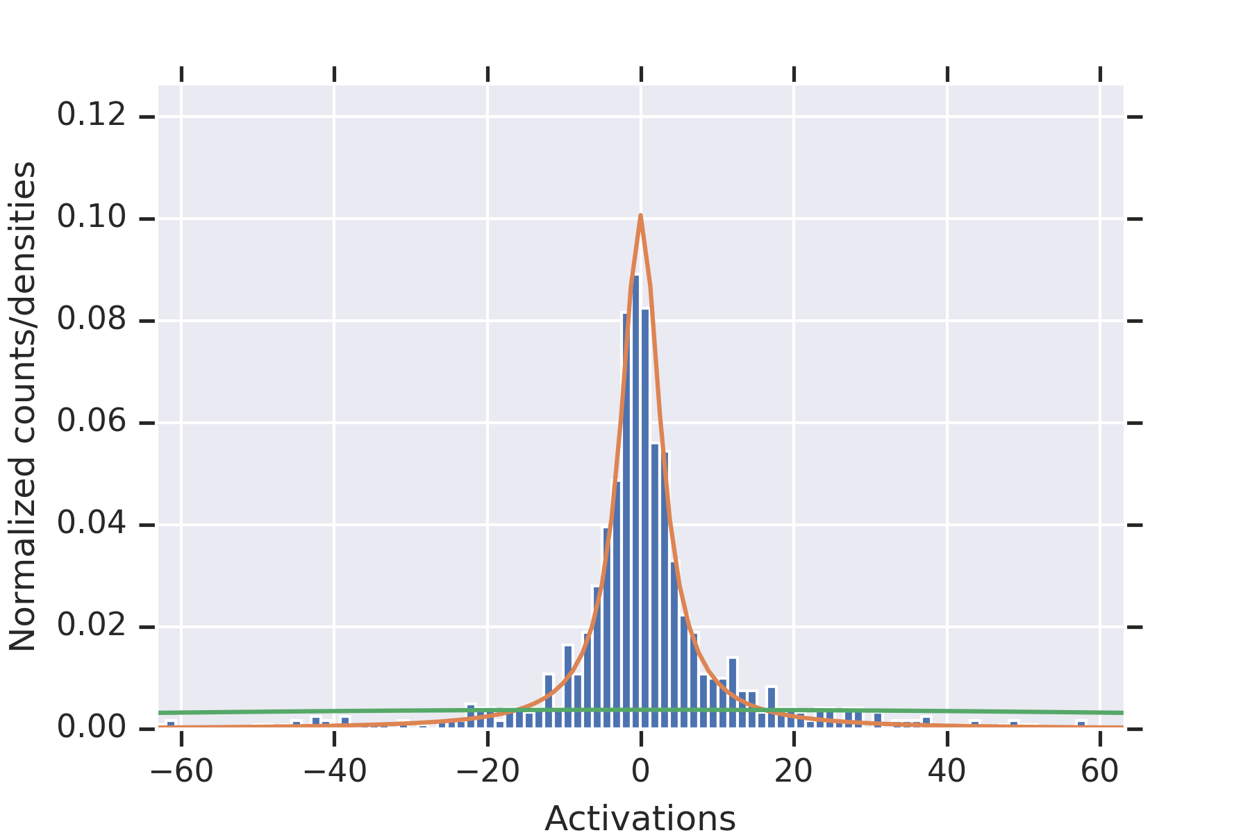 Figure 1
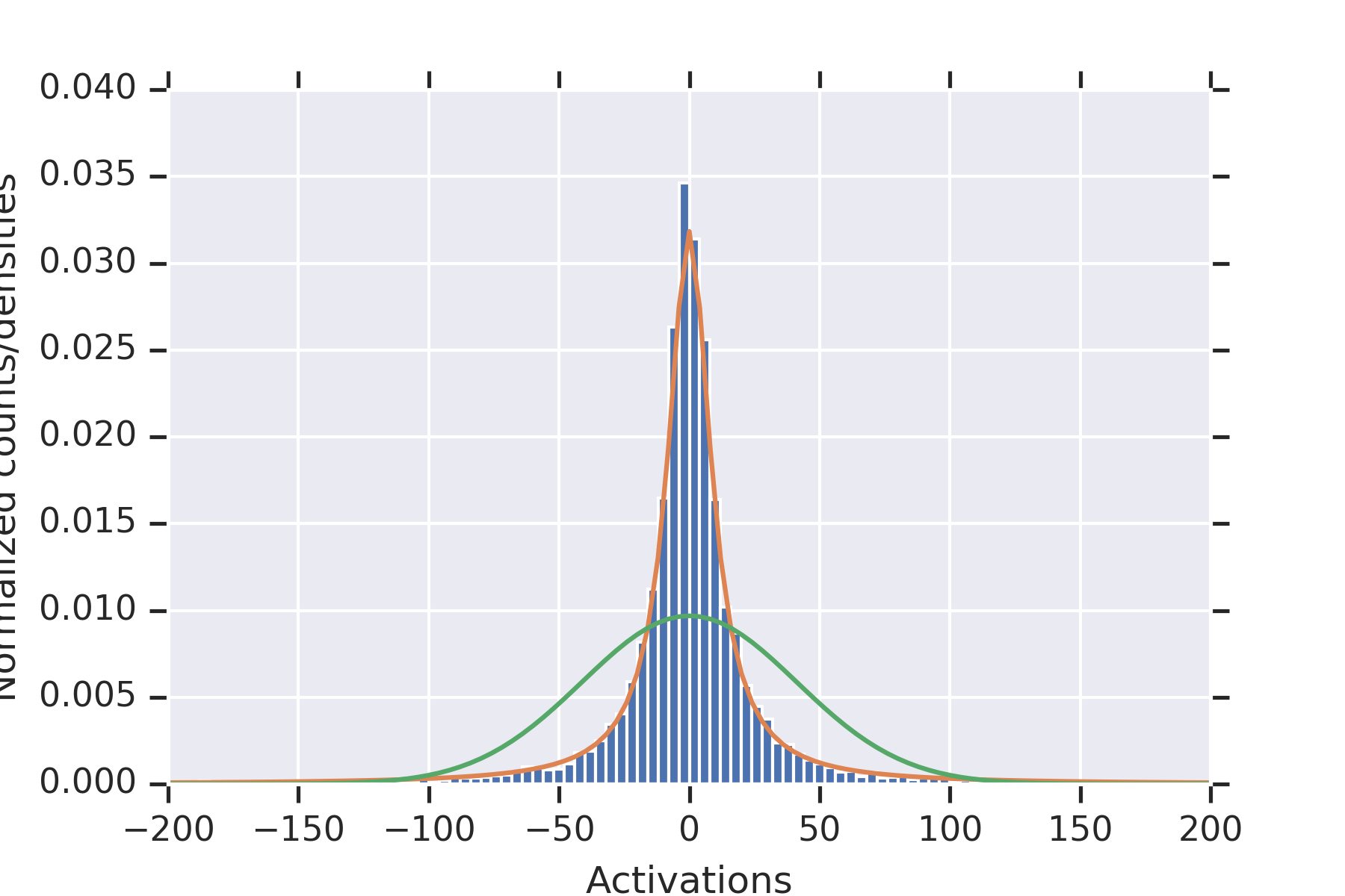 Figure 2
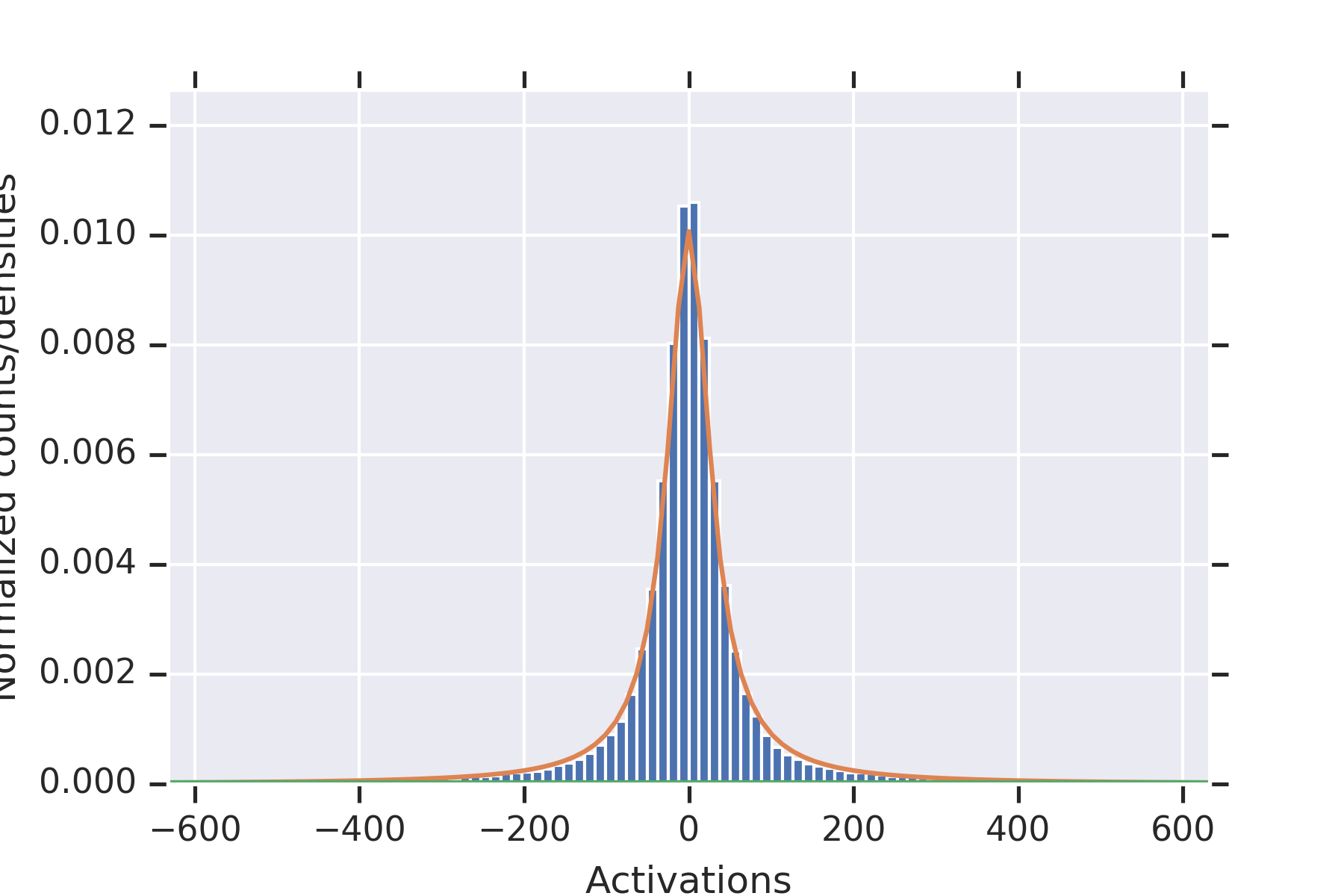 Figure 3
 Figure 4
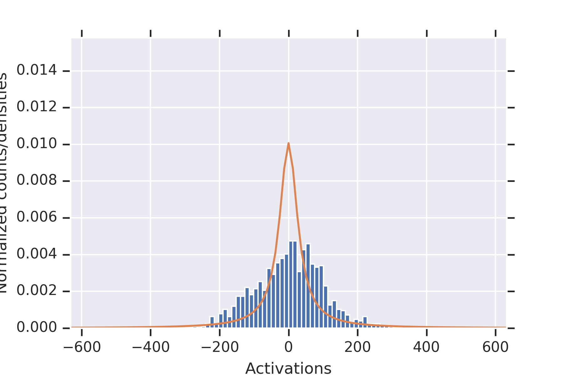 Figure 5
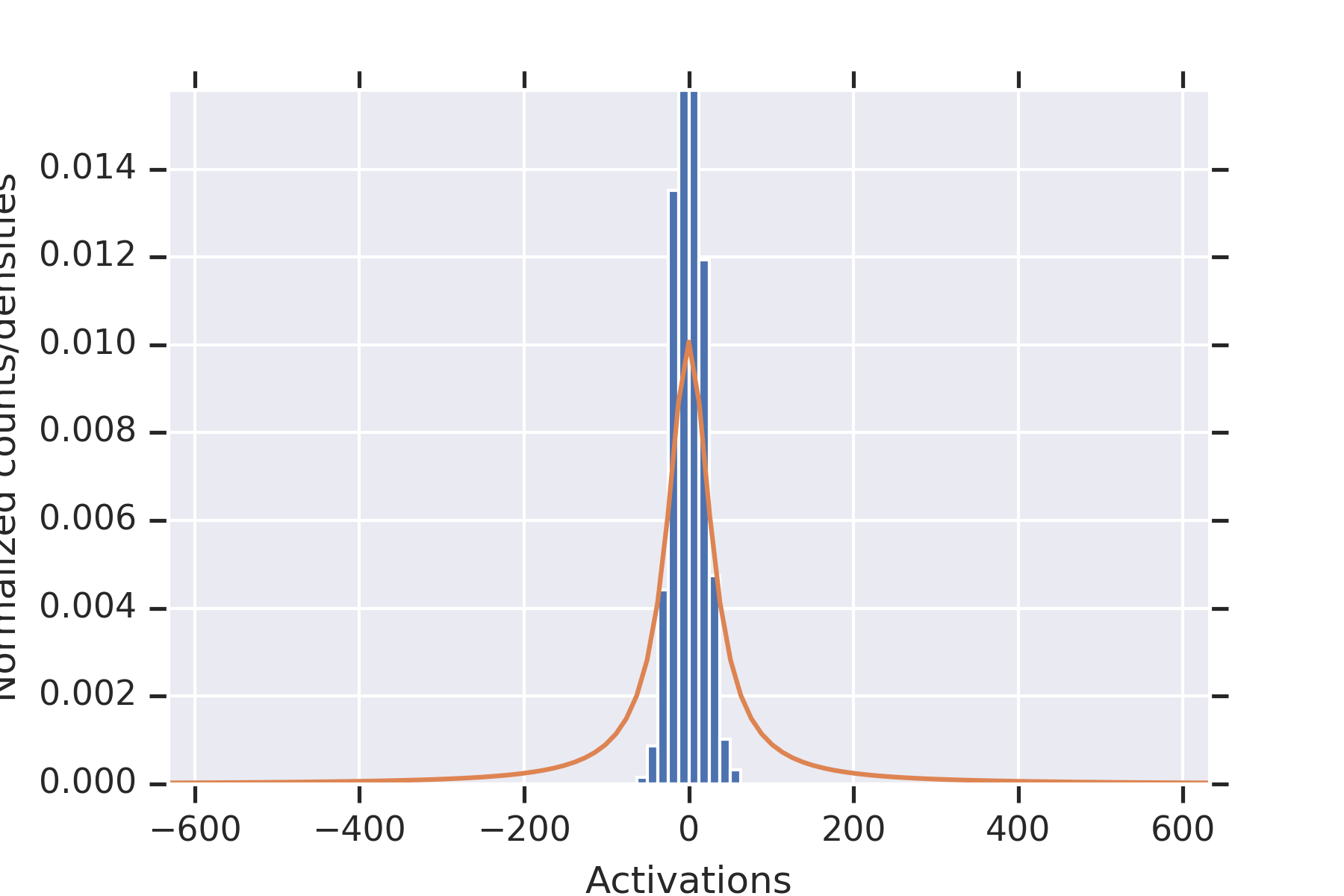 Figure 6
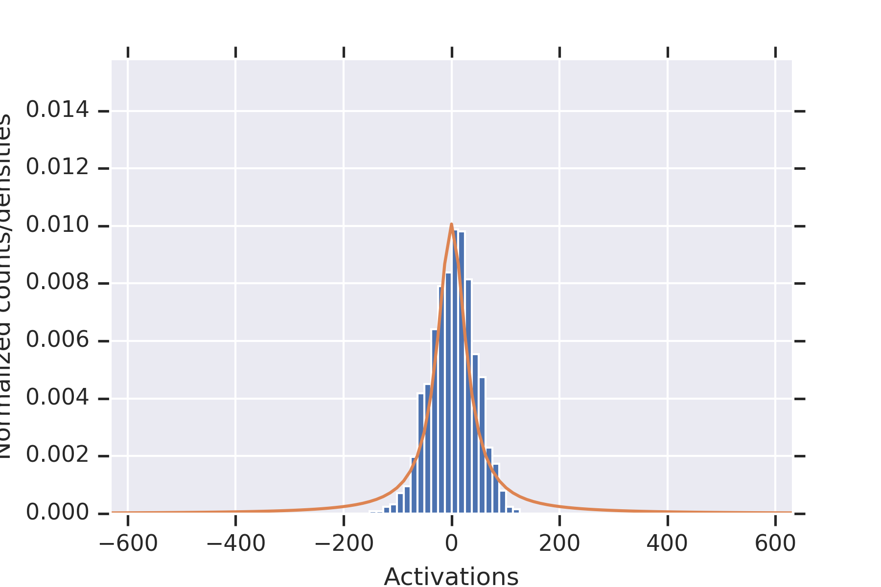 Figure 7
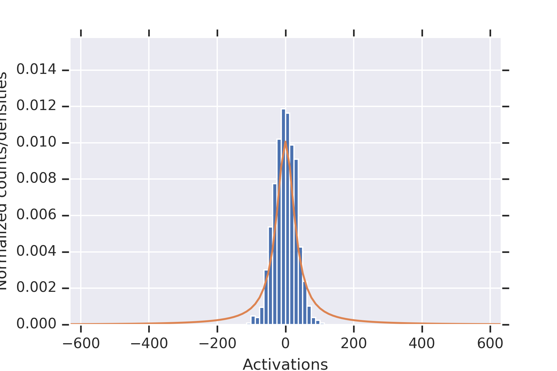 Figure 8
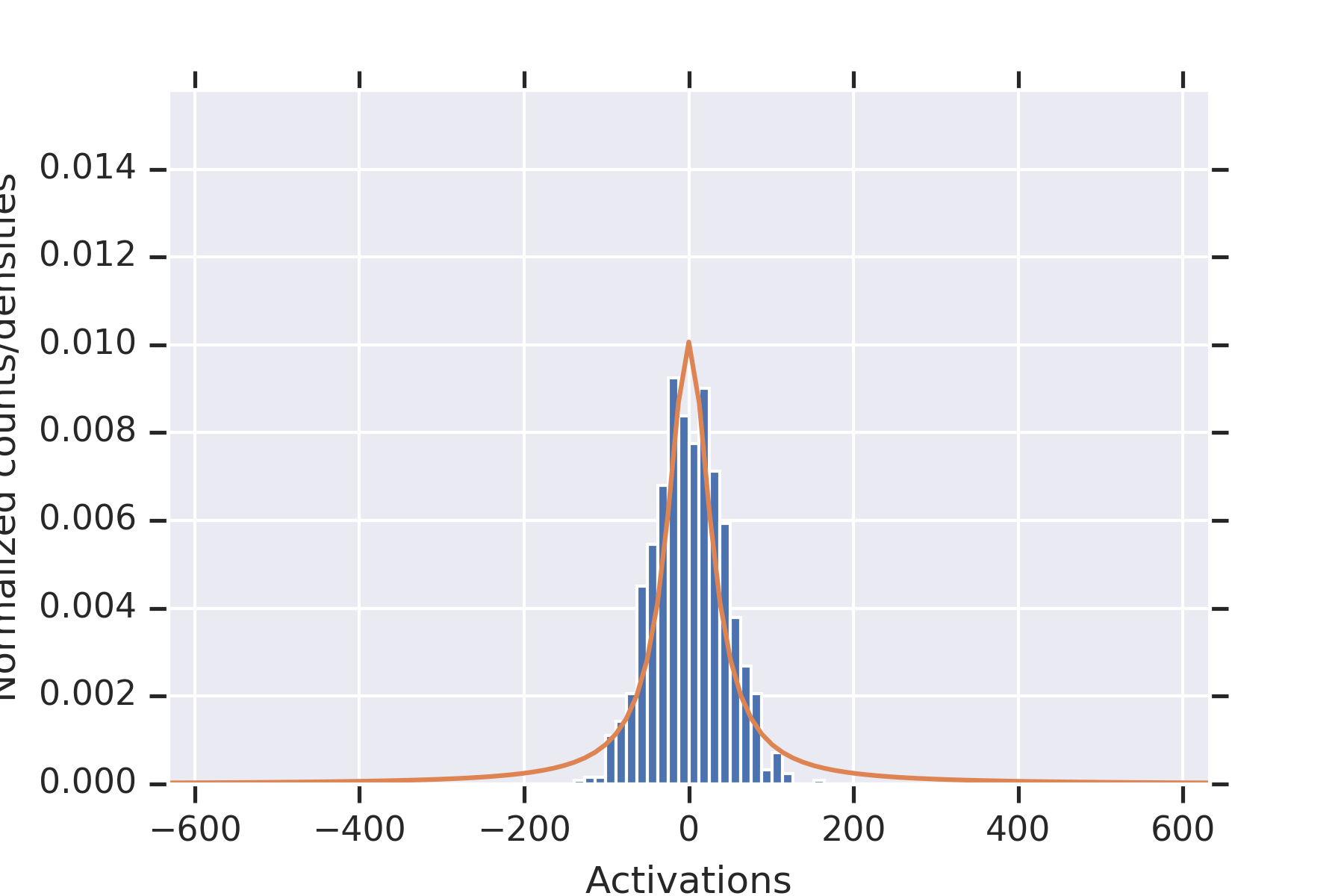 Figure 9
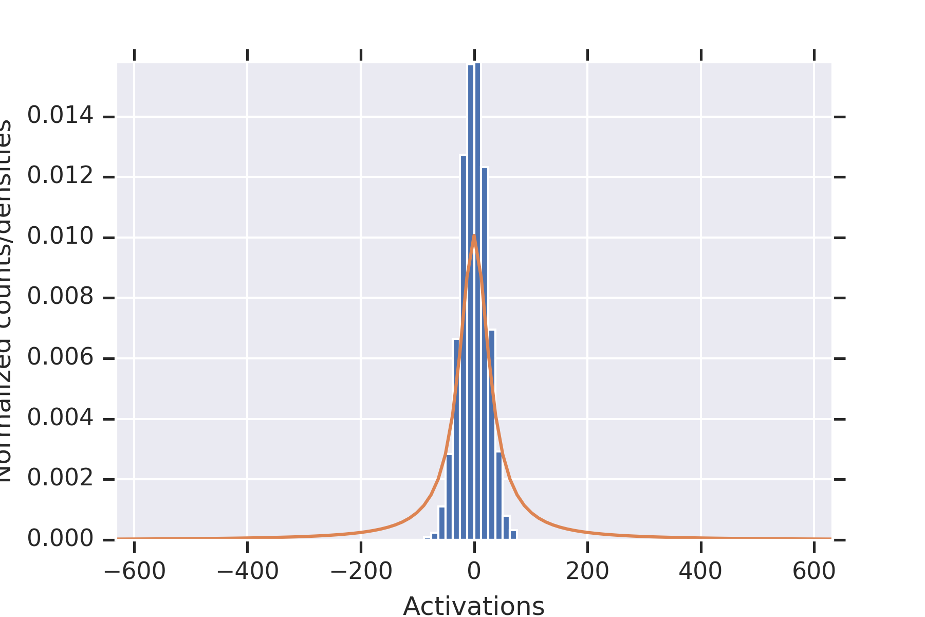 Figure 10
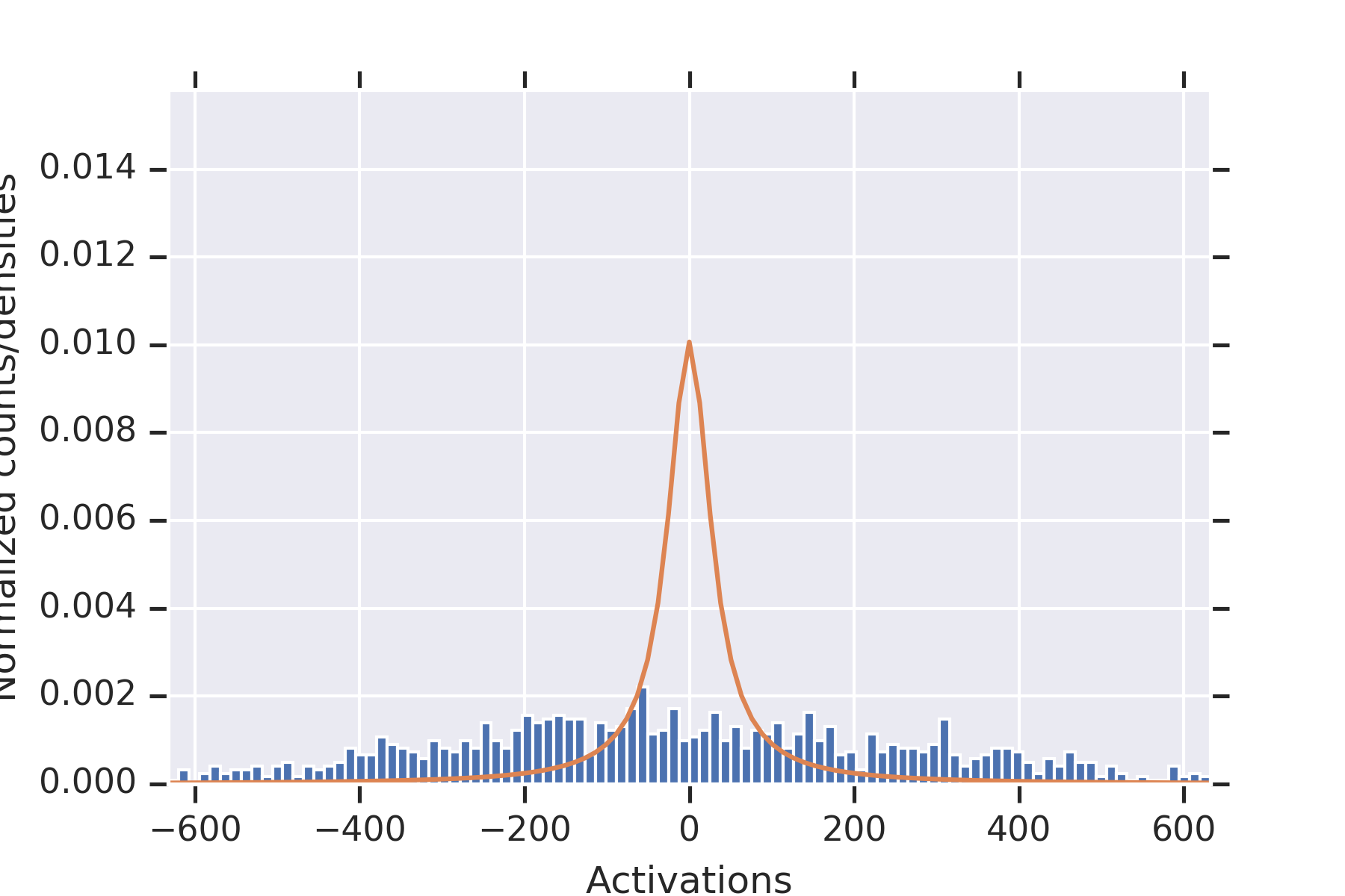 Figure 11
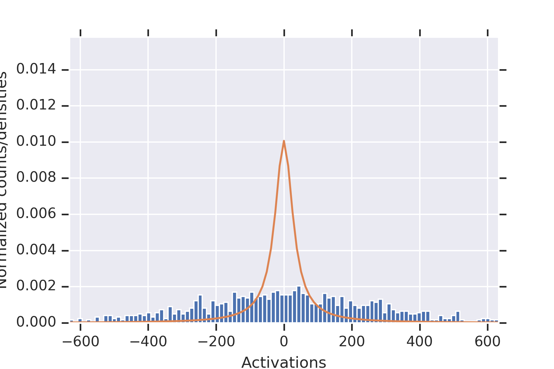 Figure 12
Peer Reviews
No public reviews on file for this paper yet. If you reviewed it on a platform where reviews are public (OpenReview, ICLR, NeurIPS, ICML), you can paste yours below so the community can read it here.
Videos
No videos yet. Explain this paper in a talk, walkthrough, or lecture? Add one.
On the effect of the activation function
on the distribution of hidden nodes
in a deep network
Philip M. Long and Hanie Sedghi11footnotemark: 1
Google Brain Authors ordered alphabetically.
Abstract
We analyze the joint probability distribution on the lengths of the vectors of hidden variables in different layers of a fully connected deep network, when the weights and biases are chosen randomly according to Gaussian distributions, and the input is in . We show that, if the activation function satisfies a minimal set of assumptions, satisfied by all activation functions that we know that are used in practice, then, as the width of the network gets large, the “length process” converges in probability to a length map that is determined as a simple function of the variances of the random weights and biases, and the activation function .
We also show that this convergence may fail for that violate our assumptions.
1 Introduction
The size of the weights of a deep network must be managed delicately. If they are too large, signals blow up as they travel through the network, leading to numerical problems, and if they are too small, the signals fade away. The practical state of the art in deep learning made a significant step forward due to schemes for initializing the weights that aimed in different ways at maintaining roughly the same scale for the hidden variables before and after a layer [9, 4]. Later work [7, 14, 2] took into account the effect of the non-linearities on the length dynamics of a deep network, informing initialization policies in a more refined way.
In this paper, we continue this line of work, theoretically analyzing what might be called the “length process”. That is, for a given input, chosen for simplicity from , we study the probability distribution over the lengths of the vectors of hidden variables, when the parameters of a deep network are chosen randomly. We analyze the case of fully connected networks, with the same activation function at each hidden node and hidden variables in each layer. As in [14], we consider the case where weights between nodes are chosen from a zero-mean Gaussian with variance , and where the biases are chosen from a zero-mean distribution with variance .
Our first result holds for activation functions that satisfy the following properties: (a) the restriction of to any finite interval is bounded; (b) as gets large,111Here denotes any function of that grows strictly more slowly than , such as for . , (c) is measurable. We refer to such as permissible. Note that conditions (a) and (c) both hold for any non-decreasing .
We show that, for all permissible and all and , as gets large, the length process converges in probability to a length map that is a simple function of , and . This length map was first discovered in [14], where it was claimed that it holds for all ; it has since been used in a number of other papers [15, 17, 12, 10, 16, 1, 13, 5].
In Section 4, to motivate our new analysis, we provide examples of that are not permissible that lead to length processes with arguably surprising properties. For example, we show that, for arbitrarily small positive , even if , for , the distribution of values of each of the hidden nodes in the second layer diverges as gets large. For finite , each node has a Cauchy distribution, which already has infinite variance, and as gets large, the scale parameter of the Cauchy distribution gets larger, leading to divergence. We also show that the hidden variables in the second layer may not be independent, even for some permissible like the ReLU. The results of this section contradict claims made in [14].
Section 5 describes some simulation experiments verifying some of the findings of the paper, and illustrating the dependence among the values of the hidden nodes.
Our analysis of the convergence of the length map borrows ideas from Daniely, et al. [2], who studied the properties of the mapping from inputs to hidden representations resulting from random Gaussian initialization. Their theory applies in the case of activation functions with certain smoothness properties, and to a wide variety of architectures. Our analysis treats a wider variety of values of and , and uses weaker assumptions on .
2 Preliminaries
2.1 Notation
For , we use to denote the set . If is a tensor, then, for , let , and define , etc., analogously.
2.2 The finite case
Consider a deep fully connected width- network with layers. Let . An activation function maps to ; we will also use to denote the function from to obtained by applying componentwise. Computation of the neural activity vectors and preactivations proceeds in the standard way as follows:
[TABLE]
We will study the process arising from fixing an arbitrary input and choosing the parameters independently at random: the entries of are sampled from , and the entries of from . For each , define .
Note that for all , all the components of and are identically distributed.
2.3 The wide-network limit
For the purpose of defining a limit, assume that, for a fixed, arbitrary function , for finite , we have . For , if the limit exists (in the sense of “convergence in distribution”), let be a random variable whose distribution is the limit of the distribution of as goes to infinity. Define and similarly.
2.4 Total variation distance
If and are probability distributions, then , and if and are their densities,
3 Convergence in probability
In this section we characterize the length map of the hidden nodes of a deep network, for all activation functions satisfying the following assumptions.
Definition 1
An activation function is permissible if, (a) the restriction of to any finite interval is bounded; (b) as gets large.222 This condition may be expanded as follows, and .; and (c) is measurable.
Conditions (b) and (c) ensure that a key integral can be computed. The proof of Lemma 1 is in Appendix A.
Lemma 1
If is permissible, then, for all positive constants , the function defined by is integrable.
Now, we recall the definition of a length map from [14]; we will prove that the the length process converges to this length map. Define and recursively as follows. First . Then, for ,
[TABLE]
and
[TABLE]
If is permissible, then, since is integrable for all , we have that are well-defined finite real numbers.
The following theorem shows that the length map converges in probability to .
Theorem 2
For any permissible , , any depth , and any , there is an such that, for all , with probability , for all , we have
The rest of this section is devoted to proving Theorem 2. Our proof will use the weak law of large numbers.
Lemma 3** ([3])**
For any random variable with a finite expectation, and any , there is an such that, for all , if are i.i.d. with the same distribution as , then
[TABLE]
In order to divide our analysis into cases, we need the following lemma, whose proof is in Appendix B.
Lemma 4
If is permissible and not zero a.e., for all , for all , and .
We will also need a lemma that shows that small changes in lead to small changes in .
Lemma 5** (see [8])**
*There is an absolute constant such that, for all ,
.*
The following technical lemma, which shows that tail bounds hold uniformly over different choices of , is proved in Appendix C.
Lemma 6
If is permissible, for all , for all , there is an such that, for all , and
Armed with these lemmas, we are ready to prove Theorem 2.
First, if is zero a.e., or if , Theorem 2 follows directly from Lemma 3, together with a union bound over the layers. Assume for the rest of the proof that is non-zero on a set of positive measure, and that , so that and for all .
For each , define
Our proof of Theorem 2 is by induction. The inductive hypothesis is that, for any there is an such that, if , then, with probability , for all , and .
The base case holds because , no matter what the value of is.
Now for the induction step; choose , and . (Note that these choices are without loss of generality.) Let take a value that will be described later, using quantities from the analysis. By the inductive hypothesis, whatever the value of , there is an such that, if , then, with probability , for all , we have and . Thus, to establish the inductive step, it suffices to show that, after conditioning on the random choices before the th layer, if , and , there is an such that, if , then with probability at least with respect only to the random choices of and , that and . Given such an , the inductive step can be satisfied by letting be the maximum of and .
Let us do that. To simplify the notation, for the rest of the proof of the inductive step, let us condition on outcomes of the layers before layer ; all expectations and probabilities will concern the randomness only in the th layer. Let us further assume that and .
Recall that . Since the values of have been fixed by conditioning, each component of is obtained by taking the dot-product of with and adding an independent . Thus, conditioned on we have that are independent. Also, since is fixed by conditioning, each has an identical Gaussian distribution.
Since each component of and has zero mean, each has zero mean.
Choose an arbitrary . Since is fixed by conditioning and and are independent,
[TABLE]
We wish to emphasize the is determined as a function of random outcomes before the th layer, and thus a fixed, nonrandom quantity, regarding the randomization of the th layer. By the inductive hypothesis, we have
[TABLE]
The key consequence of this might be paraphrased by saying that, to establish the portion of the inductive step regarding , it suffices for to be close to its mean. Now, we want to prove something similar for . We have
[TABLE]
since, recalling that we have conditioned on previous layers, are i.i.d. Since , we have
[TABLE]
which gives
[TABLE]
Since and we may choose to ensure , we have
For and to be named later, by Lemma 6, we can choose such that, for all ,
[TABLE]
and Choose such an .
We claim that for all . Choose such a . We have
[TABLE]
So now we are trying to bound using .
Using changes of variables, we have
[TABLE]
Since is permissible, is bounded on . If is the distribution obtained by conditioning on , and by conditioning on , then if , since ,
[TABLE]
But since, for , conditioning on an event of probability at least only changes a distribution by total variation distance at most , and therefore, applying Lemma 5 along with the fact that , for the constant from Lemma 5, we get
[TABLE]
Tracing back, we have
[TABLE]
which implies
[TABLE]
If , , and this implies
Recall that is an average of identically distributed random variables with a mean between [math] and (which is therefore finite) and is an average of identically distributed random variables, each with mean between [math] and . Applying the weak law of large numbers (Lemma 3), there is an such that, if , with probability at least , both and hold, which in turn implies and , completing the proof of the inductive step, and therefore the proof of Theorem 2.
4 Diversity of behavior in the distribution of hidden nodes
In this section, we show that, for some activation functions, the probability distribution of hidden nodes can have some surprising properties.
4.1 Non-Gaussian
In this subsection, we will show that the hidden variables are sometimes not Gaussian. Our proof will refer to the Cauchy distribution.
Definition 2
A distribution over the reals that, for and , has a density given by is a Cauchy distribution, denoted by . is the standard Cauchy distribution.
Lemma 7** ([6])**
If are i.i.d. random variables with a Cauchy distribution, then has the same distribution.
Lemma 8** ([11])**
If and are zero-mean normally distributed random variables with the same variance, then has the standard Cauchy distribution.
The following shows that there is a such that the limiting is not defined. It contradicts a claim made on line 7 of Section A.1 of [14].
Proposition 9
There is a such that, for every , if , then (a) for finite , does not have a Gaussian distribution, and (b) diverges as goes to infinity.
Proof: Consider defined by \phi(y)=\left\{\begin{array}[]{ll}1/y&\mbox{if y\neq 0}\\ 0&\mbox{if y=0}.\end{array}\right.
Fix a value of and , and take . Each component of is a sum of zero-mean Gaussians with variance ; thus, for all , . Now, almost surely, By Lemma 8, for each , has a Cauchy distribution, and since , recalling that , we have that are i.i.d. . Applying Lemma 7, is also .
So, for all , is . Suppose that converged in distribution to some distribution . Since the cdf of can have at most countably many discontinuities, we can cover the real line by a countable set of finite-length intervals whose endpoints are points of continuity for . Since converges to in distribution, for any , Thus, the probability assigned by to the entire real line is [math], a contradiction.
4.2 Independence
The following contradicts a claim made on line 8 of Section A.1 of [14].
Theorem 10
If is either the ReLU or the Heaviside function, then, for every , , and , are not independent.
Proof: We will show that , which will imply that and are not independent.
As mentioned earlier, because each component of is the dot product of with an independent row of plus an independent component of , the components of are independent, and since , this implies that the components of are independent. Since each row of and each component of the bias vector has the same distribution, is i.i.d.
We have
[TABLE]
The components of and , along with , are mutually independent, so terms in the double sum with have zero expectation, and For a random variable with the same distribution as the components of , this implies
[TABLE]
Similarly,
[TABLE]
Putting this together with (3), we have
[TABLE]
Now, we calculate the difference using (4) for the Heaviside and ReLU functions.
Heaviside. Suppose is Heaviside function, i.e. is the indicator function for . In this case, since the components of are symmetric about [math], the distribution of is uniform over . Thus , and so (4) gives
ReLU. Next, we consider the case that is the ReLU. Recalling that, for all , , we have By symmetry this is . Similarly, . Plugging these into (4) we get that, in the case the is the ReLU, that
[TABLE]
completing the proof.
Note that, informally, the degree of dependence established in the proof of Theorem 10 approaches [math] as gets large.
4.3 Undefined length map
Here, we show, informally, that for at the boundary of the second condition in the definition of permissibility, the recursive formula defining the length map breaks down. Roughly, this condition cannot be relaxed.
Proposition 11
For any , if is defined by , there exists a s.t. is undefined for all .
Proof: Suppose . Then , so that
[TABLE]
and downsteam values of and are undefined.
5 Experiments
Our first experiment fixed , , , .
For each , we (a) initialized the weights times, (b) plotted the histograms of all of the values of , along with the distribution from the proof of Proposition 9, and for estimated from the data.
Consistent with the theory, the distribution fits the data well.
To illustrate the fact that the values in the second hidden layer are not independent, for and the parameters otherwise as in the other experiment, we plotted histograms of the values seen in the second layer for nine random initializations of the weights in Figure 2. When some of the values in the first hidden layer have unusually small magnitude, then the values in the second hidden layer coordinately tend to be large.
Note that this is consistent with Theorem 2 establishing convergence in probability for permissible , since the used in this experiment is not permissible.
Appendix A Proof of Lemma 1
Choose . Since and , we also have
and . Thus, there is an such that, for all , , which implies . Since is permissible, it is bounded on . Thus, we have
[TABLE]
completing the proof.
Appendix B Proof of Lemma 4
The proof is by induction. The base case holds since .
To prove the inductive step, we need the following lemma.
Lemma 12
If is not zero a.e., then, for all , .
Proof: If is the Lebesgue measure, since
[TABLE]
there exists such that . For such an , we have
[TABLE]
Returning to the proof of Lemma 4, by the inductive hypothesis, , which, since , implies . Applying Lemma 12 yields .
Appendix C Proof of Lemma 6
Since there is an such that, for all , , which implies . Now, choose . For , we then have
[TABLE]
By increasing if necessary, we can ensure which then gives
. A symmetric argument yields , completing the proof.
The reference list from the paper itself. Each links out to its DOI / PubMed record.
- 1[1] M. Chen, J. Pennington, and S. S. Schoenholz. Dynamical isometry and a mean field theory of RN Ns: Gating enables signal propagation in recurrent neural networks. ar Xiv preprint ar Xiv:1806.05394 , 2018.
- 2[2] A. Daniely, R. Frostig, and Y. Singer. Toward deeper understanding of neural networks: The power of initialization and a dual view on expressivity. In Advances In Neural Information Processing Systems , pages 2253–2261, 2016.
- 3[3] W. Feller. An introduction to probability theory and its applications . John Wiley & Sons, 2008.
- 4[4] X. Glorot and Y. Bengio. Understanding the difficulty of training deep feedforward neural networks. In Proceedings of the thirteenth international conference on artificial intelligence and statistics , pages 249–256, 2010.
- 5[5] S. Hayou, A. Doucet, and J. Rousseau. On the selection of initialization and activation function for deep neural networks. ar Xiv preprint ar Xiv:1805.08266 , 2018.
- 6[6] M. Hazewinkel. Cauchy distribution. In Encyclopaedia of Mathematics: Volume 6 . Springer Science & Business Media, 2013.
- 7[7] K. He, X. Zhang, S. Ren, and J. Sun. Delving deep into rectifiers: Surpassing human-level performance on imagenet classification. In Proceedings of the IEEE international conference on computer vision , pages 1026–1034, 2015.
- 8[8] B. Klartag. A central limit theorem for convex sets. Inventiones mathematicae , 168(1):91–131, 2007.