Adaptive asynchronous time-stepping, stopping criteria, and a posteriori error estimates for fixed-stress iterative schemes for coupled poromechanics problems
Elyes Ahmed, Jan Martin Nordbotten, Florin Adrian Radu

TL;DR
This paper introduces adaptive asynchronous time-stepping and stopping criteria for fixed-stress iterative schemes in coupled poromechanics, utilizing a posteriori error estimates to improve accuracy and efficiency in simulations.
Contribution
It develops a posteriori error estimates and adaptive algorithms for fixed-stress schemes, enabling more efficient and accurate coupled poromechanics simulations.
Findings
Guaranteed and fully computable error bounds are derived.
Adaptive algorithms improve convergence and computational efficiency.
Numerical experiments confirm the effectiveness of the proposed methods.
Abstract
In this paper we develop adaptive iterative coupling schemes for the Biot system modeling coupled poromechanics problems. We particularly consider the space-time formulation of the fixed-stress iterative scheme, in which we first solve the problem of flow over the whole space-time interval, then exploiting the space-time information for solving the mechanics. Two common discretizations of this algorithm are then introduced based on two coupled mixed finite element methods in-space and the backward Euler scheme in-time. Therefrom, adaptive fixed-stress algorithms are build on conforming reconstructions of the pressure and displacement together with equilibrated flux and stresses reconstructions. These ingredients are used to derive a posteriori error estimates for the fixed-stress algorithms, distinguishing the different error components, namely the spatial discretization, the temporal…
Click any figure to enlarge with its caption.
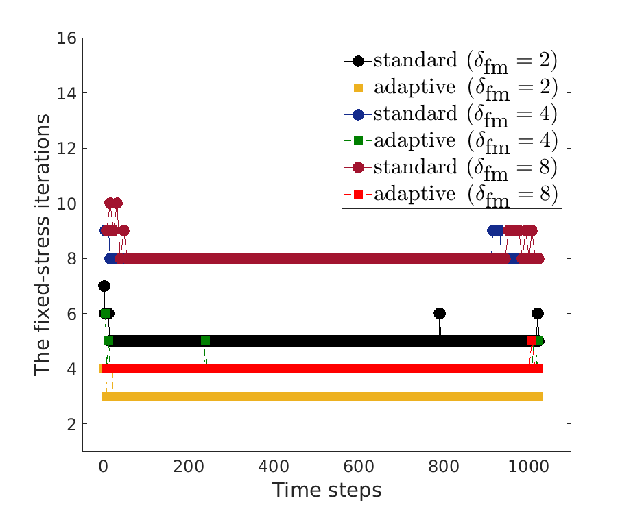 Figure 1
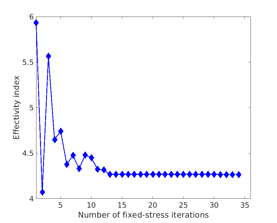 Figure 2
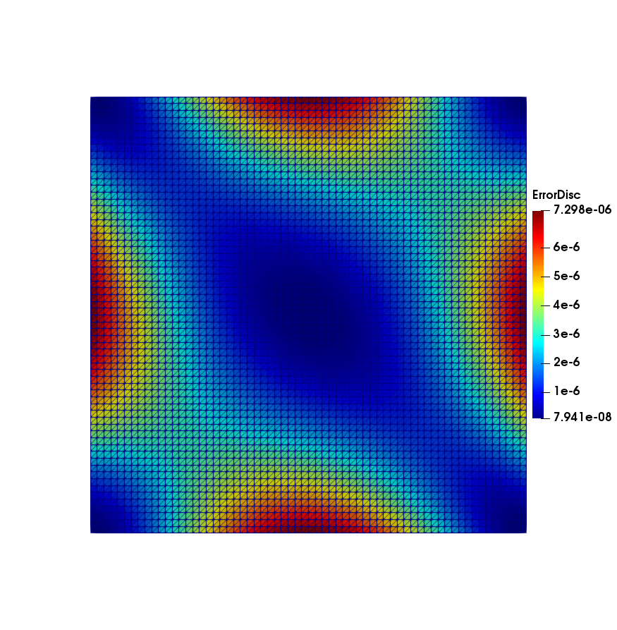 Figure 3
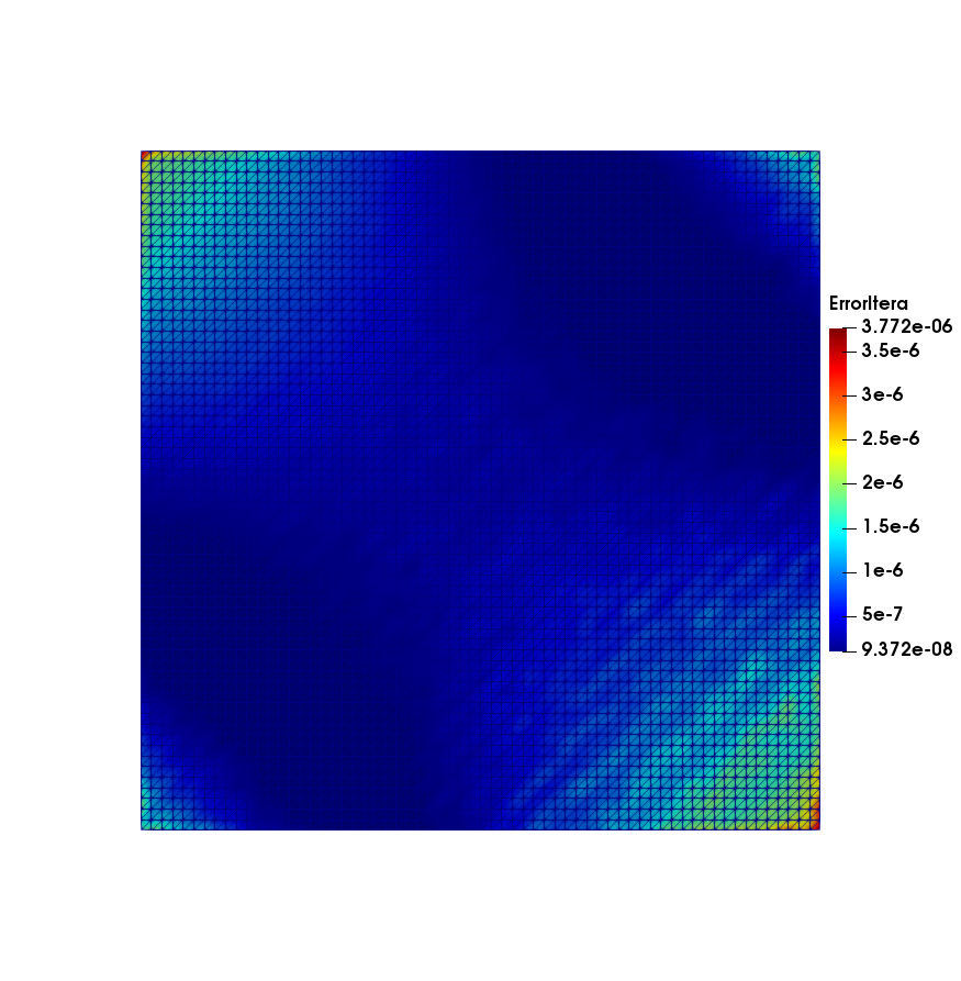 Figure 4
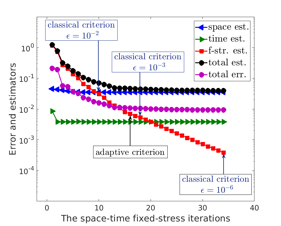 Figure 5
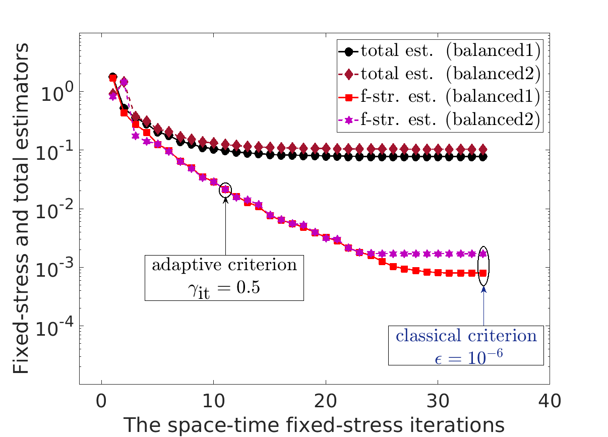 Figure 6
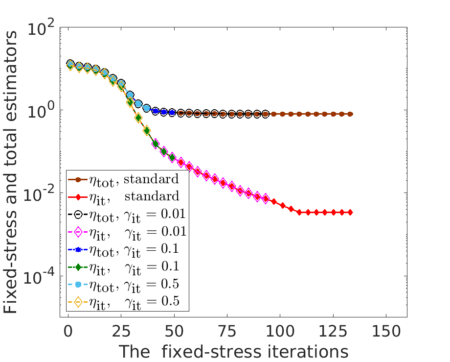 Figure 7
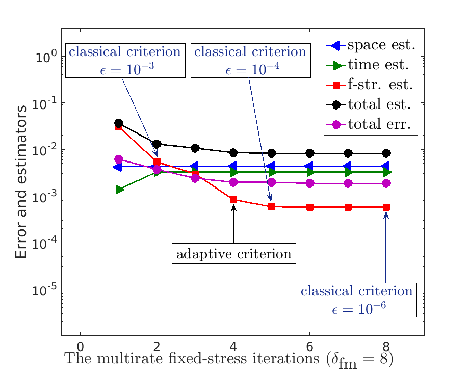 Figure 8
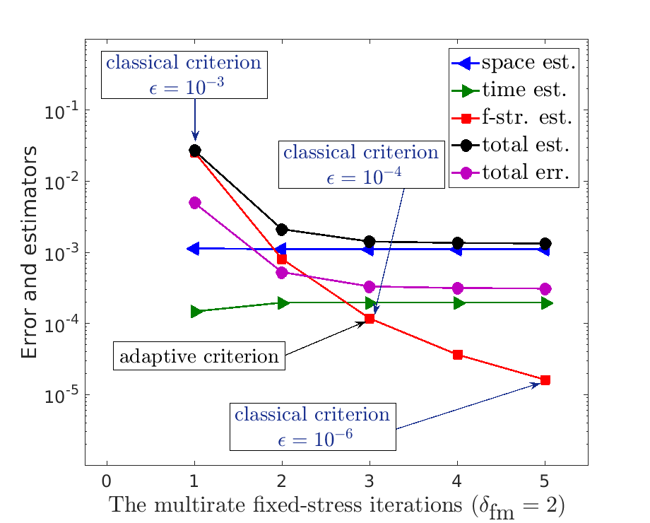 Figure 9
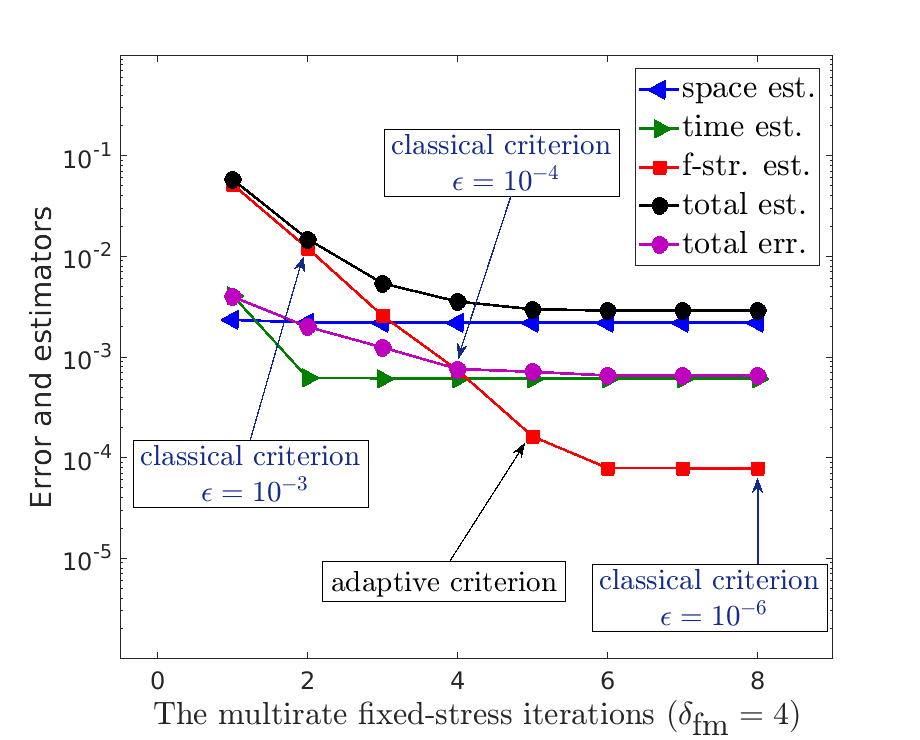 Figure 10
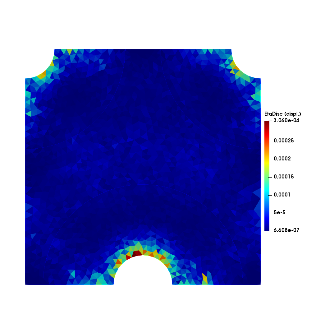 Figure 11
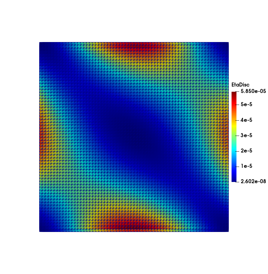 Figure 12
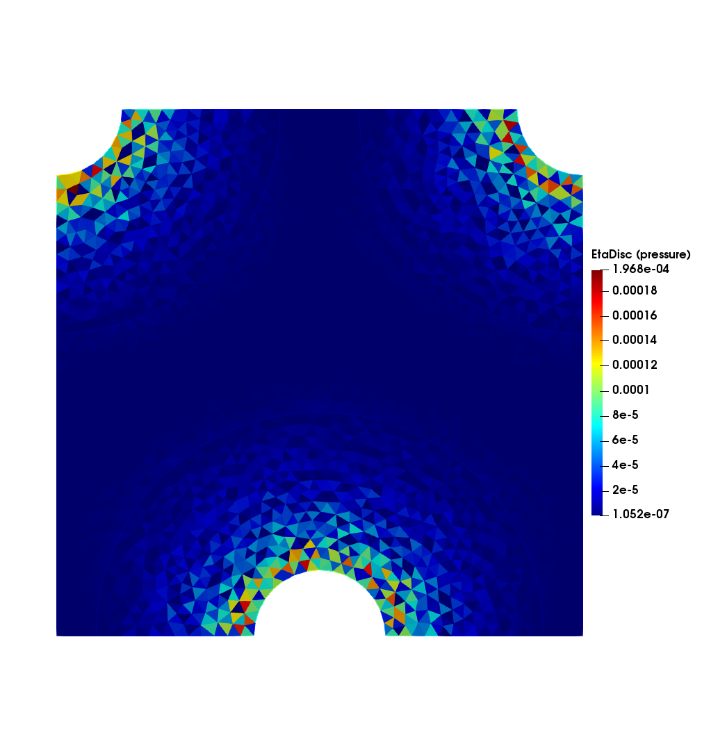 Figure 13
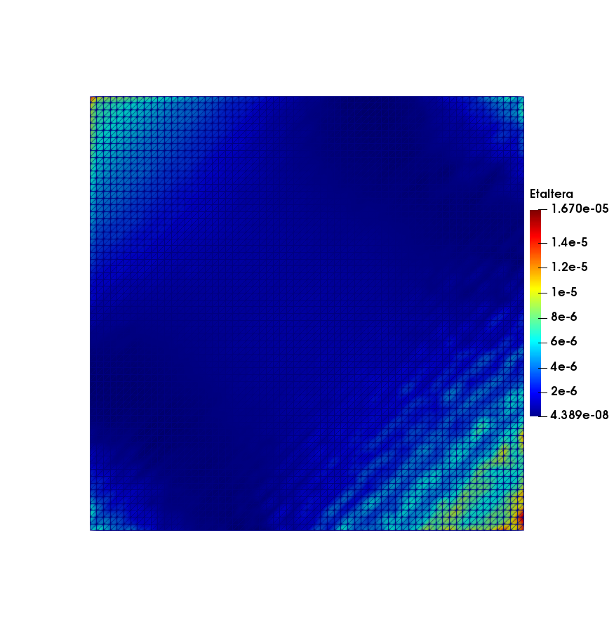 Figure 14
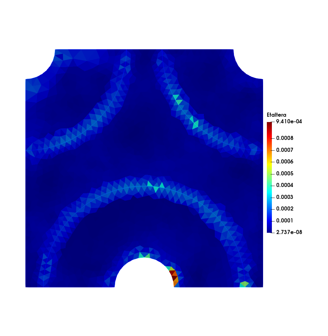 Figure 15
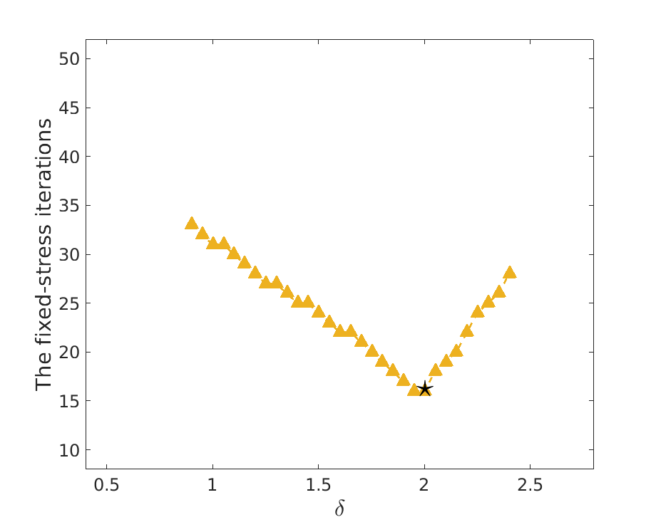 Figure 16
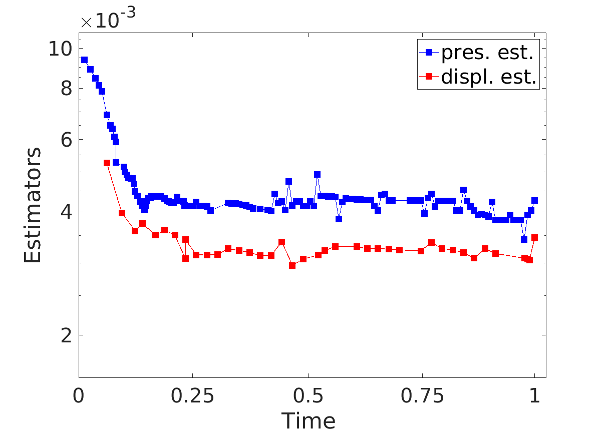 Figure 17
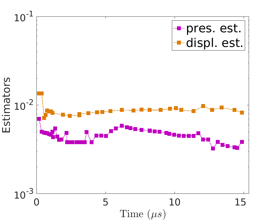 Figure 18
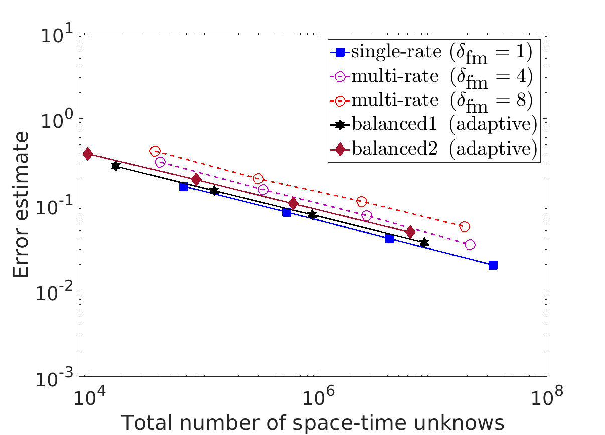 Figure 19
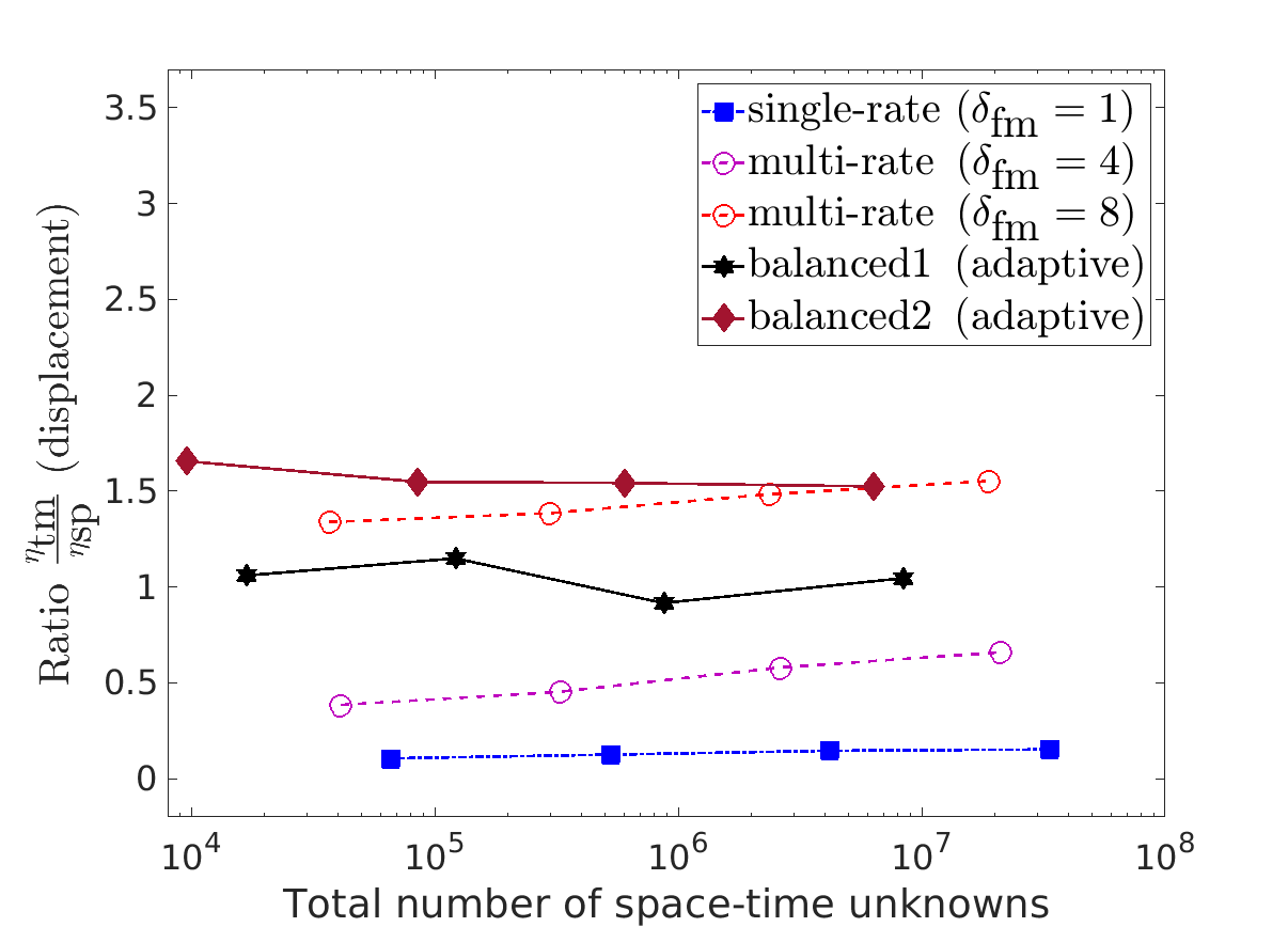 Figure 20
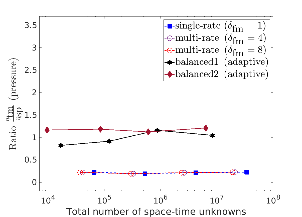 Figure 21
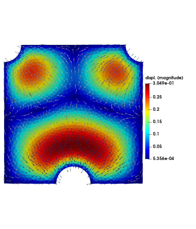 Figure 22
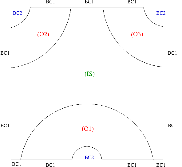 Figure 23
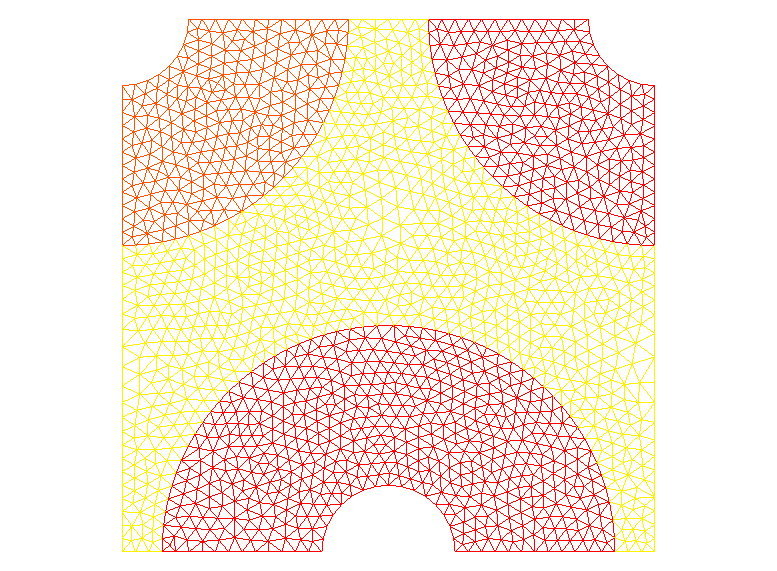 Figure 24
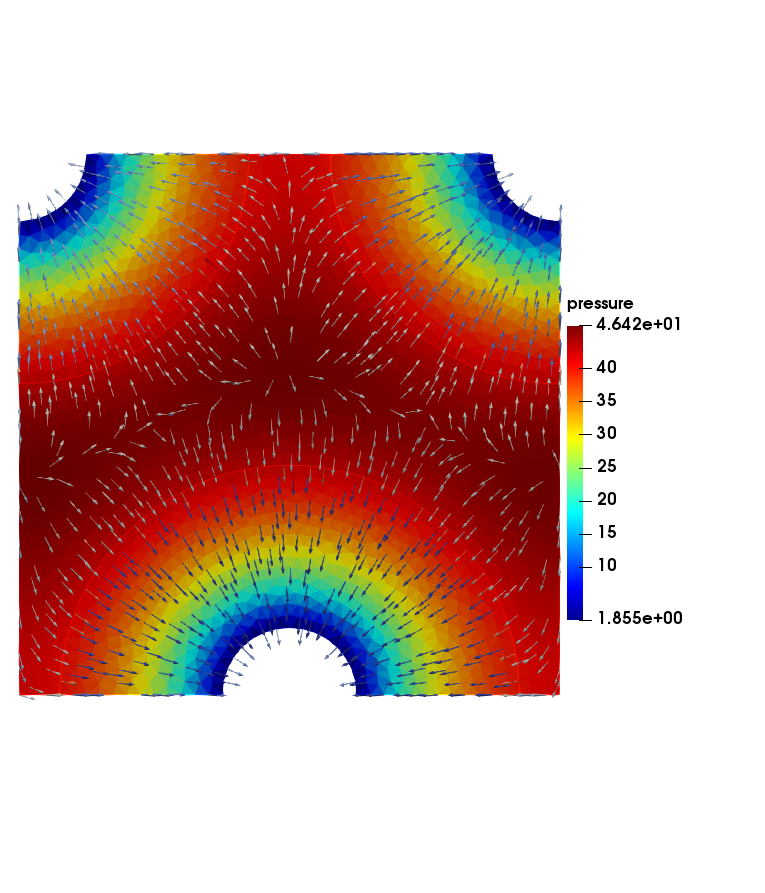 Figure 25
| Algorithm | adaptive | standard | |
|---|---|---|---|
| User-weights | , | , | none |
| Tolerance | |||
| Nb. iterations | |||
| Nb. unknowns | 571201 | 864341 | 1920375 |
| Tot. estimate | 0.7943 | 0.723 | 0.638 |
Peer Reviews
No public reviews on file for this paper yet. If you reviewed it on a platform where reviews are public (OpenReview, ICLR, NeurIPS, ICML), you can paste yours below so the community can read it here.
Videos
No videos yet. Explain this paper in a talk, walkthrough, or lecture? Add one.
Adaptive asynchronous time-stepping, stopping criteria, and a posteriori error estimates for fixed-stress iterative schemes for coupled poromechanics problems††thanks: This work forms part of Norwegian Research Council project 250223
Elyes Ahmed222Department of Mathematics, University of Bergen, P. O. Box 7800, N-5020 Bergen, Norway. [email protected], [email protected], [email protected],
Jan Martin Nordbotten222Department of Mathematics, University of Bergen, P. O. Box 7800, N-5020 Bergen, Norway. [email protected], [email protected], [email protected], 333Department of Civil and Environmental Engineering, Princeton University, Princeton, N. J., USA.
Florin Adrian Radu222Department of Mathematics, University of Bergen, P. O. Box 7800, N-5020 Bergen, Norway. [email protected], [email protected], [email protected],
Abstract
In this paper we develop adaptive iterative coupling schemes for the Biot system modeling coupled poromechanics problems. We particularly consider the space-time formulation of the fixed-stress iterative scheme, in which we first solve the problem of flow over the whole space-time interval, then exploiting the space-time information for solving the mechanics. Two common discretizations of this algorithm are then introduced based on two coupled mixed finite element methods in-space and the backward Euler scheme in-time. Therefrom, adaptive fixed-stress algorithms are build on conforming reconstructions of the pressure and displacement together with equilibrated flux and stresses reconstructions. These ingredients are used to derive a posteriori error estimates for the fixed-stress algorithms, distinguishing the different error components, namely the spatial discretization, the temporal discretization, and the fixed-stress iteration components. Precisely, at the iteration of the adaptive algorithm, we prove that our estimate gives a guaranteed and fully computable upper bound on the energy-type error measuring the difference between the exact and approximate pressure and displacement. These error components are efficiently used to design adaptive asynchronous time-stepping and adaptive stopping criteria for the fixed-stress algorithms. Numerical experiments illustrate the efficiency of our estimates and the performance of the adaptive iterative coupling algorithms.
Key words: Biot’s poro-elasticity problem; mixed finite element method; fixed-stress iterative coupling; space-time scheme; multi-rate scheme; Arnold–Falk–Winther elements; a posteriori error analysis; energy-type estimates; adaptive asynchronous time-stepping; adaptive stopping criteria.
1 Introduction
Let be an open, bounded and connected domain in , , which is assumed to be polygonal with Lipschitz-continuous boundary , and let be the final simulation time. We consider in this paper the problem of flow in deformable porous media modelled by the quasi-static Biot system [42]: find a displacement and a pressure satisfying:
[TABLE]
where is the body force and is the volumetric source term. The function denotes the effective stress tensor, i.e., , with is the linearized strain tensor given by and the operator “tr” denotes the trace of matrices. The coefficients and are the Lamé parameters, supposed strictly positive constants. The function denotes the fluid content, i.e., , where is the constrained-specific storage coefficient, and is the Biot–Willis constant. The parameter is the permeability tensor divided by fluid viscosity; it is a symmetric, bounded, and uniformly positive definite tensor whose terms are for simplicity supposed piecewise constant on the mesh of defined below and constant in time. Finally, is the initial pressure and is the initial displacement.
Throughout, we will use the convention that if is a space of functions, then we designate by a space of vector functions having each component in , and we designate by the space of tensor functions having each component in . Let ; the space is endowed with its natural inner product written with associated norm denoted by . When the domain coincides with , the subscript is dropped. Let be the Lebesgue measure of . We designate by the usual Sobolev space and by for its zero-trace subspace. Its norm and semi-norm are written and respectively. In particular, is the dual of . Further, let be the space of vector-valued functions from that admit a weak divergence in . Its natural norm is
[TABLE]
We also define to be the space of tensor-valued functions from that admit a weak divergence (by rows) in . Then, we set
[TABLE]
To give the mixed formulation of (1.1), we introduce the total stress tensor; , and the Darcy velocity; . Let , then introduce the fourth-order compliance tensor given by
[TABLE]
which is known to be bounded and symmetric definite uniformly with respect to , we can rewrite equations (1.1) in mixed weak sense:
Definition 1.1** (The five-field formulation [2]).**
Assume , , and . The fully mixed formulation of (1.1) reads: find such that
[TABLE]
together with the initial condition (1.1d).
The well-posedness and regularity analysis of the Biot equations (1.1) have been addressed in [42]. That of the existence and uniqueness of a weak solution of problem (1.3) have been addressed in [3] (see [2] for more details). Therein, two mixed formulations are discretized with the backward Euler scheme in-time and in-space with mixed finite elements methods, then a posteriori error estimates for their solutions are derived. The main issue arising when apply MFE methods for this problem is that it results a very large system to be solved at each time step (see [3, 15, 45]). This issue together with the fact that flow and mechanics effects act at different time scales, encourage the development of efficient techniques for the resolution of these coupled systems. Splitting-based iterative methods [17, 27, 31, 32] provide one such approach. They adopt the “divide and conquer” strategy and split the two systems. Then, a sequential approach is used, in that either the problem of flow or the mechanics is solved first followed by solving the other system using the already calculated information, leading to recover the original solution [28, 33, 46]. The decoupling procedure enjoys the use of a local static condensation for the flow and mechanics. The MFE system resulting from each subsystem can be reduced to a symmetric and positive definite one; pressure is the sole unknown for the flow problem, and the displacement and rotation (may also be only the displacement depending on the used quadrature rule) for the mechanics (see [6, 7] for more details). Particularly, in the last years, a lot of research has been done on the fixed-stress method [5, 13, 18, 23]. Applied to problem (1.3), it can be rewritten, as, see [11]:
Definition 1.2** (The space-time fixed-stress algorithm).**
Chose an initial approximation of and a tolerance . Set . 2. 2.
Do**
- (a)
Increase . 2. (b)
Compute such that
[TABLE] 3. (c)
Compute such that
[TABLE]
While* .*
The above method is the space-time fixed stress introduced first [13], in which we solve first the problem of flow over the whole space-time interval, then exchange the space-time information to solve the mechanics. This method is of interest for (i) the flexibility to use different time steps for flow and mechanics (ii) the advantage to derive error and a posteriori error analysis, permitting the use of adaptive asynchronous time-stepping (iii) the possibility to parallelize step 2.(c) of the algorithm. The classical fixed-stress algorithm in-space with four-field mixed formulation was analyzed in [46], where a priori convergence results are given. Other related works on this method can be found in [5, 14, 16, 23, 33] and the references therein.
In this paper, we are interested in designing adaptive versions of two common discretizations of the algorithm addressed in Definition 1.2, see Algorithm 3.1, 3.2 (standard), and Algorithm 4.2 (adaptive) below. To this aim, two iterative solution strategies for the Biot’s consolidation problem are presented; they are based on the above fixed stress iterative scheme, in which at each iteration, the space-time subsystems are solved sequentially using MFE methods in-space and with a backward Euler scheme in-time (cf. [46]). We constitute their adaptive counterpart upon the distinction of the different error components arising in the standard fixed stress algorithm, namely the spatial discretization, the temporal discretization, and the fixed stress iteration components. To arrive to this aim, we take ideas from [8, 22, 25, 29], for general a posteriori error techniques taking into account inexact iterative solvers, but most closely form [1], where a domain decomposition problem is solved via space-time iterative methods. Particularly, we will rely on [3, Theorem 6.2] where an energy-type-norm differences between the exact and the approximate pressure and displacement is shown to be bounded by the dual norm of the residuals. The developed adaptive fixed-stress algorithm is applicable on any locally conservative discretization for the two coupled subsystems, such as cell-centered finite volume scheme, multipoint mixed finite element, mimetic finite difference and hybrid high-order discontinuous Galerkin [12, 26, 37, 41]. It can also be extended to conforming methods using equilibrated flux and stress reconstructions ( cf. [40]).
In contrast to what is developed in [3], three additional features to be treated in this work; first is that the current setting targets inexact iterative coupling schemes for the Biot system and not monolithic solvers; second that the MFE methods here provides at each iteration of the coupling algorithms approximate flux and stress not balanced with the source terms; third is that the actual setting provides adaptive asynchronous time-stepping for the flow and mechanics problems. Here, we first show that the presented a posteriori error estimate delivers sharp bound (as reflected by moderate effectivity indices) for the actual energy-type error, and this at each iteration of the coupling algorithm. We also show how the overall error propagates between the flow and mechanics subproblems during the iterative process, and then to address the question of when to stop the iterations. This question was asked in [5, 11, 13], where the practitioners iterate between the two coupled subsystems until some fixed tolerance has been reached. The used stopping criterion is in fact mostly related to the algebraic error, i.e., the closeness of to the convergent solution is only taken into account without reference to the underlying continuous Biot’s problem (1.1). Here, by distinguishing the space, time and coupling errors, the adaptive stopping criterion for the iterative scheme that we propose instead is when the coupling error does not contribute significantly to the overall error. In grosso modo, the standard approach stops the iterations at some arbitrary tolerance, which hopefully is sufficiently accurate (but perhaps not!), while the approach based on error estimates stops the iterations at the correct time. Adaptive stopping criteria via a posteriori error estimates in the context of other model problems are treated in [1, 4, 19, 25], see also the references therein. Furthermore, the resulting algorithms involve tuning parameters that can be optimized (see [43]); the results show how a posteriori error estimates can help optimize these parameters. To the best of our knowledge, this combination of features in the adaptive fixed-stress algorithms is unique.
The paper is organized as follows. Section 2 fix the notation for temporal and spatial meshes and defines some relevant functional spaces. In Section 3, we present two common discretizations of Algorithm (1.4)-(1.5), by combining in-space two mixed finite elements for the flow and mechanical problems, and a backward Euler scheme in-time. As a posteriori error estimate has no meaning for piecewise constant functions, the MFE approximate pressure and displacement will be locally postprocessed in order to obtain improved approximations. In Section 4, we first introduce two major improvements to these two standards algorithms, by designing for each one, an adaptive stopping criterion, and a balancing criterion equilibrating the space and time error components using an adaptive asynchronous time-stepping. These enhancements are used to design adaptive versions of the fixed-stress schemes based on a posteriori error estimates. We then construct the needed ingredients for the a posteriori error estimates: Section 5, defines the - and conforming reconstructions. In Section 6, these ingredients are used to bound an energy-type error in the pressure and displacement at each iteration of the coupling algorithm by a guaranteed and fully computable error estimate. This a posteriori estimate is then elaborated by distinguishing the fixed-stress iterative coupling error from the space and time error components. We also separate the pressure error components from those of displacement errors. We show numerical results in Section 7. Finally, a conclusion that highlights our developments is given in Section 8.
2 Notation
We introduce here the partition of , time discretization, notation, and function spaces; see [2] for a similar notation.
2.1 Partitions of the time interval
The space-time iterative method we use supports asynchronous time grids for flow and mechanics. To this aim, the subscripts “f”, and “m” will be used throughout, to stand for flow and mechanics, respectively. For integer values , let denote a sequence of positive real numbers corresponding to the discrete flow time steps such that . Let , and be the discrete times for the flow problem. Let . For the time stepping for the problem of mechanics, we will restrict ourselves to the case in which a fixed number of local flow time steps corresponds to one coarse mechanics time step. We suppose that , with and are given positive integer values, where is the fixed number of local flow time steps within one coarse mechanics time step. We then let such that ; for . We have then , and we let , and be the discrete times for the problem of mechanics; see [5] for a similar notation. We use . For any sufficiently smooth function , we use the notation , for all .
2.2 Partition of the domain
Let be a simplicial mesh of , matching in the sense that for two distinct elements of their intersection is either an empty set or their common vertex or edge. Let denote the diameter of and be the largest diameter of all triangle; . The set of vertices of the mesh is denoted by , for the set of interior vertices, and for the set of boundary vertices. For each , let denote the patch of the vertex , i.e., all the elements which share the vertex . We denote by the corresponding open subset of .
2.3 Discrete function spaces
To approximate the flow subproblem (1.4), we let be the Raviart–Thomas–Nédélec mixed finite element spaces of order zero on the mesh (cf. [9]):
[TABLE]
where denotes the lowest-order Raviart–Thomas–Nédélec finite-dimensional subspace associated with the element .
To approximate the mechanics subproblem (1.5), we let be the Arnold–Falk–Winther mixed finite elements with weakly symmetric stress for the lowest-order stresses on the mesh (cf. [10]):
[TABLE]
where denotes the subspace of composed of skew symmetric–valued tensors.
Let be a space of functions defined on . We denote the vector space of functions continuous in time and with values in . We also denote by the space of functions piecewise constant in time and with values in . We have then if , then is such that for all ,
[TABLE]
3 Fully discrete space-time fixed-stress schemes based on MFE in-space
and the backward Euler scheme in-time
In this section, we provide two discretization of Algorithm (1.4)-(1.5) using the backward Euler scheme in-time, and in-space, using two mixed finite elements methods for the linear elasticity and flow problems. A post-processing routine is then given to preview the numerical pressure and displacement solutions.
3.1 Two standard discrete fixed-stress schemes.
In the first algorithm, we consider the case of equal time grids for the flow and mechanics problems, i.e., . The fully discrete form of Algorithm 1.2 reads then as follows:
Algorithm 3.1** (The global-in-time fixed-stress).**
Chose an initial approximation of , a real constant , and a tolerance . Set . 2. 2.
Do**
- (a)
Increase and set . 2. (b)
Do**
- i.
Increase . 2. ii.
Approximate , the solution to
[TABLE]
While* .* 3. (c)
Reset . 4. (d)
Do**
- i.
Increase . 2. ii.
Approximate , solution to
[TABLE]
While* .*
While* . \[email protected]*
We present now the nonconforming-in-time counterpart of Algorithm 1.2 in the spirit of multi-rate fixed-stress scheme specified in [5]:
Algorithm 3.2** (The nonconforming-in-time (multi-rate) fixed-stress).**
Chose an initial approximation of , a real constant , and a tolerance . Set . 2. 2.
Do**
- (a)
Increase and set . 2. (b)
Do**
- i.
Increase and set . 2. ii.
Do**
- A.
Increase . 2. B.
Approximate , solution to
[TABLE]
While* .* 3. iii.
Approximate , solution to
[TABLE]
While* . \[email protected]*
While* .*
Remark 3.3** (The multi-rate FS).**
The convergence of the multi-rate fixed-stress was shown in [5] where mixed finite element method is used for the flow equations and where the mechanics is solved by conformal Galerkin method. Therein, the algorithm is also limited to one coarser time step for the mechanics and there is no study on the propagation of error due to temporal and spatial discretizations.
Remark 3.4** (Space-time vs multi-rate).**
We first notice that Algorithm 3.2 is practical to problems with a long time integration interval; In contrast to Algorithm 3.1, it requires reasonable computation ability and less storage resources to handle large-scale applications. Furthermore, Algorithm 3.2 is exploiting the different time scales for the flow and mechanics subsystems. We note also that the efficiency of the two algorithms can be improved when the free parameter is well-chosen (see [43]) and that step 2.(d) of Algorithm 3.1 in practice, is done in parallel as in [13].
3.2 Post-processing
We do here some improvements to the approximate solution (cf. [21, 30]). This step is also mandatory to design from Algorithm 3.1 and 3.2, their adaptive versions based on energy-norm-type a posteriori error estimate. This is customary in mixed finite elements schemes, as an energy-norm-type a posteriori error estimate has no meaning for the piecewise constant, i.e., .
Let us notice first that in Algorithm 3.2, the approximate solution of the mechanics problem is defined in different time grids from the approximate flow solution , so we cannot proceed to the post-processing of the displacement and the reconstruction of the stress tensor unless we build the couple at the finer time steps , for all , and for all . To this aim, we construct the displacement and the stress tensor as follows: for , we set
[TABLE]
Note that this post-processing is explicit and its cost is negligible. The post-processing of the pressure is as follows [21, 30, 24]: at each iteration , we calculate the improved solution in each element such that
[TABLE]
This post-processing is computationally cheap and easy to be implemented. We then extend this post-processing (cf. [30]) to the vector case, leading to define a function , such that
[TABLE]
where denotes the -th Euclidean unit vector. We finally assume for simplicity that the initial conditions are satisfied exactly, i.e.,
[TABLE]
We define the continuous and piecewise affine in–time functions and by
[TABLE]
The key observation in the above post-processing is that they use only local operations, which are independent from each other and hence parallelizable.
4 The adaptive fixed-stress algorithms
The purpose of this section is to reduce as much as possible the computational effort of Algorithm 3.1 and 3.2 as in [1, 4, 20, 22]. The improvements of these two standards algorithms stems from (i) important savings in terms of the number of coupling iterations can be achieved using adaptive stopping criterion (ii) a significant gain in the computational resources is obtained by balancing the error components via an asynchronous adaptivity of the temporal meshes (iii) optimizing the tuning parameter .
4.1 Methodology for adaptive asynchronous time-stepping and adaptive stopping criteria
Let , and , for , be respectively the estimators of the spatial discretization error, the temporal discretization error and the fixed-stress coupling error at the time step and on the iteration, where the index J=P is for the pressure error components, and that of J=U is for the displacement error components. We let .
The first step of our developments is to equip Algorithm 3.1 and 3.2 with adaptive asynchronous time-stepping. To this aim, we propose to equilibrate the time errors with the spatial errors as follows; we adjust the time steps and so that
[TABLE]
where and , are user-given weights, typically close to .
An alternative to (4.1) being to balance the time errors from the flow and mechanics discretization with the global error by selecting the time steps and in such a way that
[TABLE]
The balancing criterion (4.1) controls the contributions of and in the overall error and leads to . That of the second criterion (4.2) leads to equilibrate the time errors from the flow and mechanics, i.e., .
The second step of our developments is to equip Algorithm 3.1 and 3.2 with adaptive stopping criteria. We then introduce a real parameter to be given in . The stopping criteria for Algorithm 3.1 is chosen at each iteration as
[TABLE]
which implies that we stop the iterations if the coupling error is sufficiently lower than one of the other components. The stopping criteria for Algorithm 3.2 is set similarly: at each coarse mechanics time step , at each iteration ,
[TABLE]
Remark 4.1** (Algebraic errors).**
The systems within the flow and mechanics subsystems are solved with direct solvers. The present adaptive approach can also be combined with an iterative solver for each subproblem, and to further save computational effort, these latter can be stopped whenever the algebraic errors does not contribute significantly to the overall error, following [25].
4.2 The adaptive algorithms
We are now ready to present the adaptive counterparts of Algorithm 3.1 and 3.2, i.e., they are now equipped with adaptive asynchronous time-stepping and a posteriori stopping criterion. The adaptive version of Algorithm 3.1 is as follows:
Algorithm 4.2** (Adaptive Fixed-Stress with Asynchronous Time Mesh Refinement and Adaptive Stopping Criteria ).**
In step 1, chose also a real parameter and the real weights and , set , and give an initial ratio and time step for the flow and the temporal refinement threshold . Set . 2. 2.
Do**
- (a)
Increase and set . 2. (b)
Do**
- i.
Increase . 2. ii.
Set . 3. iii.
Approximate by (3.1). 4. iv.
Calculate the estimators , and . Check the balancing criterion (4.1) (or (4.2)). If not satisfied, refine or redefine the flow time step in such a way that condition (4.1) (or (4.2)) holds or , and return to step 2.(b)iii. 5. v.
Set .
While* .* 3. (c)
Reset and , and let . 4. (d)
Do**
- i.
Increase . 2. ii.
Set . 3. iii.
Approximate by (3.2). 4. iv.
Calculate the estimators , and . Check the balancing criterion (4.1) (or (4.2)). If not satisfied, redefine the time step for the mechanics using using in such a way that condition (4.1) (or (4.2)) holds, and return to step 2.(d)iii. 5. v.
Set .
While* .*
Until* the criteria (4.3) is satisfied.*
Similarly, we propose to modify Algorithm 3.2. This yields to an adaptive fixed-stress scheme equivalent to Algorithm 4.2 but applied through temporal windowing technique. Precisely, the whole time interval is now split into time-windows , . Algorithm 4.2 is first applied on the first time window . Afterwards, one applies the algorithm on the next time window imposing as initial condition for the solution of the converged iterate of the end of the previous time window and proceeds in such a way until all time windows have been treated.
Remark 4.3** (Space adaptivity).**
The estimators are calculated on each element of the mesh and on each time step, and could also be used as indicators in order to refine adaptively the spatial mesh , so that the local spatial error estimators are distributed equally; see [3, 20, 44] and the references therein. Furthemore, the efficiency of the adaptive algorithms can be enhanced by using adaptive multiscale meshes, where two spatial meshes for the flow and mechanics subsystems are considered and where they are refined/coarsened adaptively in order to equilibrate the space errors for the two subsystems; see the multiscale discretizations techniques in [18, 38].
Remark 4.4** (Static condensation).**
The decoupling procedure permits the use of a local static condensation for the flow and mechanics and then to reduce the MFE system resulting from each subproblem to a symmetric and positive definite one; for the pressure for the flow problem, and for the displacement and rotation for the mechanics problem; with the same way as in [6, 7]. These systems are smaller and easier to solve than the original saddle point problems, but no further reduction is possible.
Remark 4.5** (Computational cost).**
In practice, the adaptive time-stepping strategy is only done in the first or second iterations of the Algorithm. Further, when the step size is modified once at current time step, the updated step size can be used for some subsequent time steps, say for example time steps. Then on the sixth time step, step 2.(b)iv is checked again if the step size needs to be modified for the next time steps. Furthermore, steps 2.(b)iv and 2.(d)iv can be done only every few iterations of the Algorithm.
5 Concept of -, and -conforming reconstructions in Biot’s poro-elasticity system
In this section, we develop basic tools that will allow us to build the estimators involved in the adaptive fixed-stress algorithms.
5.1 Pressure and displacement reconstructions
We first construct from , a -conforming function satisfying the mean value constraint
[TABLE]
To this aim, we proceed as in [21]; from the available post-processed pressure at each iteration , we set
[TABLE]
Here are the Lagrangian nodes situated in the interior of , denotes the standard (time-independent) bubble function supported on , defined as the product of the barycentric coordinates of , for all , and scaled so that its maximal value is 1, and is the interpolation operator given by
[TABLE]
At the Lagrange nodes situated on the boundary , we set . In order to guarantee that the mean value constraint (5.1) holds true, we choose
[TABLE]
The same procedure can be applied to the post-processed displacement . This leads to a -conforming vector function , satisfying the following mean value constraint:
[TABLE]
We end up with continuous and piecewise affine in–time functions and by setting
[TABLE]
An interesting result of the above reconstructions is given in the following Lemma (cf. [3]):
Lemma 5.1** (Properties of ).**
At each iteration of Algorithm 4.2, let be the post-processed pressure and displacement, and be the reconstructed pressure and displacement. Then, for all , there holds
[TABLE]
5.2 Equilibrated flux and
stress reconstructions
The second ingredient for the derivation of our a posteriori error estimates is to reconstruct an equilibrated flux , locally conservative on the mesh :
[TABLE]
and to reconstruct an equilibrated stress , locally conservative on the mesh :
[TABLE]
These reconstructions are based on solving local Neumann problems by mixed finite elements posed over patches of elements around mesh vertices (cf. [21, 22, 40]). For each vertex , we introduce the mixed Raviart–Thomas finite element spaces posed on the patch domain :
[TABLE]
We then introduce the Arnold–Falk–Winther mixed finite elements spaces, posed on the patch domain , for all :
[TABLE]
We obtain the equilibrated velocity field , by solving first for , for all , such that
[TABLE]
For the equilibrated stress , we solve local Neumann mechanics problems by mixed finite elements, with weakly symmetric stress: find , for all , such that
[TABLE]
The above local problems are well-posed owing to the properties of mixed finite elements (cf. [9, 10]). We can easily observe that the computational cost of the flux and stress reconstructions can be substantially reduced by pre-processing, a step that is fully parallelizable.
6 The a posteriori error estimates
We derive in this section, based on the previous constructions, a posteriori error estimates for the solution of Algorithm 3.1 or 3.2. This is done by bounding an energy error between the exact weak solution of problem (1.1) and the approximate solution , by a guaranteed and fully computable upper bound, and this at each iteration of Algorithm 3.1 or 3.2.
6.1 The error measure
The first question in a posteriori error estimates is that of the error measure; here we will in particular rely on [3, Theorem 6.2], where an energy-type error in the pressure and displacement is shown to be bounded by the dual norm of the residuals, and where the Biot’s consolidation equations (1.3), (1.1c) are discretized using MFE method in-space and with a backward Euler scheme in-time and solved monolithically. To this aim, and for all times , we let
[TABLE]
and introduce the energy space
[TABLE]
Then, we introduce a weak formulation of (1.1): find such that and and such that
[TABLE]
where denotes the duality pairing between and . The existence and uniqueness of the solution to this problem was addressed in [3]. Still following [3], we introduce the following energy-type error measure
[TABLE]
The above norms are well-defined owing to the properties of the weak solution and the reconstructed functions , i.e., we have both and in .
6.2 The error estimators
Before formulating our estimators, we define the broken Sobolev space as the space of all functions such that , for all . The energy semi-norm on is given by
[TABLE]
where the sign denote the element-wise gradient, i.e., the gradient of a function restricted to a mesh element . The energy norm in is given by
[TABLE]
We also recall the Poincaré inequality:
[TABLE]
where is the mean value of the function on the element given by and whenever the element is convex. In what follows, we denote respectively by and the smallest and the largest eigenvalue of the tensor in . We introduce the local residual estimators
[TABLE]
the flux estimators
[TABLE]
the pressure nonconformity estimators
[TABLE]
Therefrom, we introduce the global versions by
[TABLE]
6.3 Guaranteed reliability
We now provide a guaranteed estimate on the total error in particular valid on each iteration of Algorithm 3.1 or 3.2. This result extend the results of our previous work [3, Section 5], where a computable guaranteed bound on the energy-type error between the exact solution and its approximation with an exact solver has been derived.
Theorem 6.1** (Global-in-time a posteriori error estimate).**
Let be the weak solution of (6.1). At an arbitrary iteration of Algorithm 3.1 or 3.2, let be the post-processed pressure and displacement of subsection 3.2, be the reconstructed pressure and displacement and be the reconstructed flux and stress of section 5. Then, there holds
[TABLE]
where
[TABLE]
Notice that we have set and , and for ,
[TABLE]
Proof.
Recalling (6.2a), and (3.10), we have from [3, Theorem 6.2], for any given couple ,
[TABLE]
featuring the residuals and of the weak formulation (6.1): for all and ,
[TABLE]
The dual norms of the residuals are given by
[TABLE]
At each iteration , the approximate solution is not an element of , contrarily to the reconstructed solution, i.e., . Thus, to use (6.12), we apply the triangle inequality to get
[TABLE]
where we can bound the first term of the right-hand side using (6.12). What remains is to give a computable upper bound for the residuals and together with and then combine these results.
1) A computable upper bound for and . Proceeding as in [2, 40], adding to (6.13), choosing with and applying the Green theorem, and using (5.6), we obtain
[TABLE]
Then, it can be inferred using (6.15) and the Poincaré inequality (6.5) followed by Cauchy-Schwarz inequality that
[TABLE]
We repeat the same steps for (6.14), by adding and subtracting (we replace by due to symmetry), using (5.7) and applying the Poincaré inequality (6.5) together with the Cauchy-Schwarz inequality and definition (6.16), we obtain
[TABLE]
Replacing (6.19) and (6.20) in (6.12), so we are left to bound the third and fourth terms of the right-hand side of 6.12. Using the fact that (also ) is a nondecreasing function of the time , we easily obtain from (6.19)-(6.20),
[TABLE]
In a similar way, we infer
[TABLE]
and similarly
[TABLE]
We use (6.19)–(6.23) in (6.12), thus we bound the first term of (6.17):
[TABLE]
2) A computable upper bound to . To bound this term presenting the nonconformity estimator, we proceed as in [3, Theorem 5.3 Lemma 5.7], we promptly arrive to
[TABLE]
The estimate (6.10) is obtained by replacing (6.24) and (6.25) in (6.17). ∎
6.4 An a posteriori error estimate distinguishing the space, time and fixed-stress coupling
errors
Our goal in this section is to distinguish the different error components. Particularly, we separate the iterative coupling error from the estimated space and time errors, which are predefined and used efficiently in Algorithm 4.2. To this purpose, at each iteration , we define for all , the local spatial, temporal and iterative coupling estimators
[TABLE]
Therefrom, we introduce like in (6.9), ,
[TABLE]
and then introduce their global versions like in (6.11) by
[TABLE]
where for and .
Remark 6.2** (Fixed-stress estimator).**
In the above estimators, we have to mention that, for conforming time discretization, the iterative coupling estimators , J=U, P, tends to zero when the fixed-stress algorithm converges. However, this is not true for non-conforming time discretization as in the multi-rate algorithm or the adaptive one. Precisely, at each iteration , the reconstructed flux and stress are satisfying respectively the local mass conservation (5.10) and (5.11) which is not the case for the approximate flux from (3.4) and the approximate stress from (3.5) (step 2.(b)ii in Algorithm 3.2 and step 2.(b)iii in Algorithm 4.2) and this is even when the fixed-stress converges. In other words, the fixed-stress estimator becomes a non-conformity in-time estimator when the fixed stress algorithm converges.
Lemma 6.3** (A posteriori error estimate distinguishing error components).**
Let the assumptions of Theorem 6.1 be satisfied. Then there holds
[TABLE]
Proof.
We add and subtract the discrete fluxes in the flux estimator (6.7a) then apply the triangle inequality yield, for all ,
[TABLE]
Another triangle inequality leads to
[TABLE]
In the same way, we obtain for the stress estimator (6.7b), for all ,
[TABLE]
In these two inequalities, the first terms in the right-hand side form the contributions of the pressure and displacement in the fixed-stress error, whereas the second ones contribute to the two components of the space discretization error. The last terms can be integrated in time, yielding to the two components of the time error. What remains is to replace (6.31) and (6.32) in (6.10) with the use of (6.26)–(6.28), where we used the equality of norms in (6.31), i.e., , leading to the estimate (6.29). ∎
7 Numerical results
In this section we illustrate the efficiency of our theoretical results on numerical experiments. We have chosen two examples designed to show how the adaptive fixed-stress scheme behaves vs the standard ones and this is done on different physical and geometrical situations.
7.1 Test problem 1: an academic example
with a manufactured solution
We consider in the computational domain and the final time . The analytical solution of Biot’s consolidation problem is supposed to be:
[TABLE]
The effective parameters are , and . This analytical solution which has homogeneous initial and Dirichlet boundary values for and , generates from (1.1a)- (1.1b) non-zeros source terms and .
7.1.1 Stopping criteria balancing the error components
The aim here is to illustrate the performance of the adaptive stopping criteria introduced in Section 4.1. To this purpose, we consider a uniform space-time mesh with , and . The tuning parameter is chosen , with . The choice of the parameter is theoretically calculated in [11, 43, 32] and possibly should lead to the best performance of the fixed-stress method in terms of number of iterations. We first test the performance of the space–time fixed stress algorithm (Algo. 3.1) equipped with an adaptive stopping criteria. Therein, we set and compare the results with the standard approach in which the fixed-stress algorithm is continued until the algebraic residual-based criteria (2) is satisfied for an (arbitrary) threshold .
Figure 1(a) displays the dependence of the total error and of the various estimators on the fixed-stress iterations, where various stopping criteria are used. We can see that the space (blue) and time (green) estimators remain constant during the computation in contrast to the fixed-stress estimator, which gives a numerical indication that the error components are distinguished. For the fixed-stress estimator (red), we can see that the adaptive stopping criteria (4.3) is satisfied after 16 iterations only, while the classical one (2) needs 34 iterations with , 18 iterations with , and only 10 iterations with . We can remark that the total error (magenta) and the total estimator (black) decrease rapidly for the first 12 fixed-stress iterations, after which they decrease very slowly, as the influence of the fixed-stress iteration error becomes negligible. This is exactly the point where our adaptive fixed-stress method stops. This results in a significant saving of fixed-stress iterations as well as excludes possible inaccurate solutions from the algorithm (like with .) As an example, we make a gain of of total fixed-stress iterations compared to the classical algorithm with .
As known, the number of iterations to achieve convergence for the fixed-stress can differ considerably depending on the choice of the tuning parameter . Thus, in Figure 1(b), we plot the number of iterations required by the fixed-stress algorithm as function of the parameter . Therein, we stop the algorithm when the adaptive stopping criteria is satisfied. Clearly, the estimator behaves very similarly to what is usually observed for the fixed-stress error (see, e.g., [43]). Moreover, the theoretical parameter (marked by a star) coincides with the numerically optimal value. In Figure 2, we display the spatial distribution of the different error components (left) and of the corresponding estimators (right) at the final time . Clearly, the distribution of the estimated errors reflects the exact ones. Also as expected, we observe in Figure 2(d) that the estimated fixed-stress error is sufficiently small to not contribute significantly in the overall error.
In Figure 3, the effectivity index for the space–time fixed stress approach is presented. It is calculated by the ratio between the total estimator and the exact total error at the iteration of the fixed-stress algorithm. The effectivity index oscillates during the first 10 iterations, then decreases to approximately 4.27 and then remains constant until the end of the computation. One of the reasons of why this factor is far from 1, may be that the negative norms involved in the exact error are not calculated. Another explanation is that in practice, we use estimate (6.29) instead of (6.10) where the different error components are not yet separated.
In the second set of experiments, we study the performance of the adaptive stopping criteria on the multi-rate fixed-stress algorithm (MFS). Here, we compare the results with the classical multi-rate algorithm in which the algebraic residual-based criteria (2b) is used with various threshold .
In Figures 4(a)–4(c), we plot the evolution of the total error and the various estimators on the fixed-stress iterations for the final coarse mechanics step. There, we compare the adaptive to the standard multi-rate algorithm for various ratios of discretization in time, . We remark that (i) the discretization in space estimator (blue) as well as the discretization in time estimator (green) are approximately constant in each case (ii) the discretization in time estimator goes up and approaching from the discretization in space estimator when we increase the ratio . Note that the discretization in space estimator is the same for the different ratios if it is scaled with the time steps. These findings confirm numerically that we have practically distinguished the time discretization error from the spatial discretization error. Concerning the fixed-stress estimator, we recall that in that case, mixes fixed-stress and nonconformity-in-time errors (see Remark 6.2). Thus, we observe for the case , and that, dominates the total error until iteration 2 or 3, then becomes smaller than and until iteration 4 or 5, and therefrom remains constant as the influence of the fixed-stress iteration error becomes negligible compared to the nonconformity-in-time error. For , the nonconformity error is small enough so as not to contribute in until convergence. For the cases, and , we can see that the classical multi-rate fixed-stress equipped with (2b) as stopping criteria needs in the last coarse mechanics step 8 iterations to converge, and between 8 and 9 iterations for the previous ones. For , the classical algorithm needs 5 iterations to converge, and between 5 and 7 for the previous ones. For all the cases, the adaptive stopping criterion guarantees that the fixed-stress algorithm converged to the correct solution compared to the classical criteria (see the results with ), while saving a substantial amount of computational effort (see the results with and ); see the overall performance in the three cases depicted in Figure 4(d) comparing the standard approaches with to the adaptive ones.
7.1.2 Adaptive time-stepping balancing the space and time errors
In the second part of this test case, we verify the impact of the balancing criteria (4.1)-(4.2) on the fixed-stress schemes. The balancing criteria (4.1) aims adapting the times steps for the flow and mechanics subsystems in such a way that their spatial and temporal error estimators (6.26) are equilibrated through the computation. This leads practically to having . That of the criteria (4.2) equilibrates the time errors from the mechanics and flow discretizations, i.e., . Next, we will see that using the balancing (4.1) or (4.2) is important for the efficiency of the adaptive algorithm.
To this aim, we compare on three levels of uniform space-time mesh refinement, the standard space-time (Algo. 3.1 ) and the single- and multi-rate (Algo. 3.2) with algorithms with the adaptive fixed-stress one (Algo. 4.2). For the three refinement levels, we use the same weights and , J=P, U. In Figure 5 (top), the ratio of the time discretization error over the space discretization error from the flow (left) and from the mechanics (right) as a function of the total number of space–time unknowns is depicted for the aforementioned standard and adaptive algorithms. These results confirm numerically that we have distinguished the pressure and displacement errors as well as their time and space discretizations. Precisely, we can easily see that for the multi-rate schemes, the ratio (Figure 5 (top left)), remains constant when changing the ratio , in contrast to the ratio (Figure 5 (top right)), where the ratio increases with . The effect of the resulting ratios on the overall estimate is shown in Figure 5 (bottom left). These results make it evident that the performance of the fixed-stress algorithms is considerably improved if they are equipped with the balancing criteria (4.1) (balanced1) or (4.2) (balanced2). Particularly, the standard multi-rate algorithm reduces the computational cost of the single-rate one, but still much more expensive than the adaptive ones. In average, the adaptive one reduces the computational cost of the multi-rate one with while the efficiency of the algorithm in terms of precision is much more preserved. In Figure 5 (bottom right), we chose the third refinement level, then we plot the dependence of the total and fixed-stress estimators as a function of the fixed-stress iterations for the adaptive algorithms. This result confirms that the algorithm is improved if it is equipped with the balancing criteria (4.1) or (4.2). Precisely, these balancing ensure that the contribution of the fixed-stress estimator in the overall error becomes quickly negligible (see Figure 1(a) for the case without adaptivity), thus we can stop the fixed-stress iterations by setting . Furthemore, with either of these balancing criteria we have keeping a small non-conformity in-time error which makes the application of adaptive stopping criteria more comfortable and guaranteed. Note that in the standard algorithms (as shown in the results of subsection 7.1.1), the time steps and the ratio are mainly based on intuition and this may induce an over-refinement in-time and may increase the nonconformity-in-time errors, affecting considerably the efficiency of the fixed-stress algorithm. In Figure 6, we plot the pressure and displacement estimators as a function of the adaptive time steps. Note that if the developed algorithm is equipped with asynchronous adaptivity in space, we can significantly reduce the total computational cost, but also the total error, as this later is dominated by the space error from the discretization of the flow subsystem.
7.2 Test problem 2: a poro-mechanical behavior of an osteonal tissue
In this test case, the poroelastic model is carried out to study the hydro-mechanical behavior of an idealized osteonal tissue. This idealized structure is a group of osteons surrounded by their cement lines and embedded in the interstitial bone matrix [34, 35]. The simplified domain presents the parts of three different osteons connected by the interstitial system (IS): a half osteon (O1) is located at the bottom of the picture and two quarters of osteons (O2) and (O3) are placed on the top-left and top-right corners, respectively (see Figure 7).
The used material properties as generated in [36] (see also [39]) are in the osteons and in the (IS)-domain. The remaining parameters are , , , and . The boundary conditions are and on the portion BC1 and together with , and on BC2. The final time is .
We use Algorithm 4.2 equipped with (4.1) where we consider two computations that differ by the balancing parameters and . We start with an initial time step , and . The estimators are computed every 3 iterations to reduce the computational cost. Table 1 compares the number of space–time unknowns (number of asynchronous time steps, counting repetitions in the adaptive algorithm, fixed space unknowns) and performed fixed-stress iterations, and the values of the error estimators of the three computations. We observe that the gain in the number of fixed-stress iterations as well as in the number of unknowns is significant. Indeed, the two adaptive computations need approximately 30 fixed-stress to converge while the standard fixed-stress algorithm needs more than 132 iterations, thus, the total computational cost is reduced of for the first adaptive computation and of for the second one.
To clarify this gain, we can observe in Figure 8 (left) that as soon as we perform fixed-stress iterations, the fixed-stress estimator is sufficiently small to not contribute significantly on the overall error. Also as expected, the adaptive stopping criterion stops the fixed-stress algorithm when the solution is sufficiently accurate. Figure 8 (left) confirms also the role of the adaptivity in time, with which, the fixed-stress estimator becomes quickly smaller than the space and time discretization estimators, even with a large value of , for example . We can also observe that even with a small parameter , the gain in the number of fixed-stress iterations is significant. In Figure 8 (right), we plot the pressure and displacement estimators as a function of time. Clearly, the displacement error dominates the pressure error along the simulation. In Figure 9, we plot the approximate solution at the final time . Figure 10 compares the spatial discretization errors for the pressure (top left) and displacement (top right), and the fixed-stress estimator (bottom), after using our adaptive stopping criteria at the final time . Besides detecting the dominating error at the circular boundary of the Osteons, we can see that the total error is dominated by the mechanics discretization error, and that the fixed-stress estimator is negligible.
8 Conclusion
We proposed in this paper adaptive fixed-stress iterative coupling schemes for the Biot system. Our adaptive algorithm can be used either globally-in-time or (partially) via time windowing techniques, and works as follows:
- •
At the first iteration, both time step size of flow and mechanics will be adapted in such a way that the space and time error contributions are equilibrated.
- •
We then continue iterating, where several estimators (space, time and fixed-stress) are computed, until the fixed-stress estimator becomes smaller (up to a user-chosen constant) than the other error components.
The numerical experiments demonstrated the accuracy of the estimated quantities while highlighting the applicability of the presented adaptive algorithm. Particularly, the algorithm saves important number of iterations, reduces significantly the total computational cost by adapting asynchronously the flow and mechanics time-steps and avoiding over-in-time refinement together with maintaining a small non-conformity in-time error. The algorithm may also help optimizing the tuning parameter. These benefits, together with the fact that we, a posteriori, estimate the overall error that is guaranteed and without unknown constant, leads to efficient and optimized adaptive fixed-stress coupling algorithm. Note that the present approach can be extended easily to other inexact coupling methods such as drained split, undrained split, and fixed-strain split methods. Also, the present algorithm can be applied directly, without further developments to any flux- and stress-conforming discretizations of the flow and mechanics such that cell-centered finite volume or mimitic finite difference and can easily be extended to conforming methods.
Acknowledgment
The research is supported by the Norwegian Research Council Toppforsk project 250223 (The TheMSES project: https://themses.w.uib.no).
The reference list from the paper itself. Each links out to its DOI / PubMed record.
- 1[1] E. Ahmed, S. Ali Hassan, C. Japhet, M. Kern, and M. Vohralík , A posteriori error estimates and stopping criteria for space-time domain decomposition for two-phase flow between different rock types . working paper or preprint, June 2017, https://hal.inria.fr/hal-01540956 .
- 2[2] E. Ahmed, F. A. Radu, and J. M. Nordbotten , Adaptive poromechanics computations based on a posteriori error estimates for fully mixed formulations of biot’s consolidation model , research report, Department of Mathematics, University of Bergen, Nov. 2018, https://hal.inria.fr/hal-01687026 .
- 3[3] E. Ahmed, F. A. Radu, and J. M. Nordbotten , Adaptive poromechanics computations based on a posteriori error estimates for fully mixed formulations of biot’s consolidation model , Computer Methods in Applied Mechanics and Engineering, (2018), doi: https://doi.org/10.1016/j.cma.2018.12.016 , http://www.sciencedirect.com/science/article/pii/S 0045782518306145 . · doi ↗
- 4[4] S. Ali Hassan, C. Japhet, and M. Vohralík , A posteriori stopping criteria for space-time domain decomposition for the heat equation in mixed formulations , Electron. Trans. Numer. Anal., 49 (2018), pp. 151–181, doi: 10.1553/etna_vol 49s 151 , https://doi.org/10.1553/etna_vol 49s 151 . · doi ↗
- 5[5] T. Almani, K. Kumar, A. Dogru, G. Singh, and M. F. Wheeler , Convergence analysis of multirate fixed-stress split iterative schemes for coupling flow with geomechanics , Comput. Methods Appl. Mech. Engrg., 311 (2016), pp. 180–207, doi: 10.1016/j.cma.2016.07.036 , https://doi.org/10.1016/j.cma.2016.07.036 . · doi ↗
- 6[6] I. Ambartsumyan, E. Khattatov, J. M. Nordbotten, and I. Yotov , A multipoint stress mixed finite element method for elasticity i: Simplicial grids , ar Xiv preprint ar Xiv:1805.09920, (2018).
- 7[7] I. Ambartsumyan, E. Khattatov, J. M. Nordbotten, and I. Yotov , A multipoint stress mixed finite element method for elasticity ii: Quadrilateral grids , ar Xiv preprint ar Xiv:1811.01928, (2018).
- 8[8] M. Arioli, D. Loghin, and A. J. Wathen , Stopping criteria for iterations in finite element methods , Numer. Math., 99 (2005), pp. 381–410, doi: 10.1007/s 00211-004-0568-z , https://doi.org/10.1007/s 00211-004-0568-z . · doi ↗