A Markov jump process modelling animal group size statistics
Pierre Degond, Maximilian Engel, Jian-Guo Liu, Robert L. Pego

TL;DR
This paper models animal group size dynamics using a Markov jump process derived from coagulation-fragmentation equations, enabling numerical approximation of equilibrium states and analysis of statistical properties, with connections to stochastic differential equations.
Contribution
It formalizes a coagulation-fragmentation model as a Markov jump process and develops a numerical scheme for equilibrium approximation, extending previous models with new analytical and simulation insights.
Findings
Validated numerical scheme matches analytical equilibrium results.
Analyzed population and size distributions for complex rates.
Established connection between jump processes and stochastic differential equations.
Abstract
We translate a coagulation-framentation model, describing the dynamics of animal group size distributions, into a model for the population distribution and associate the \blue{nonlinear} evolution equation with a Markov jump process of a type introduced in classic work of H.~McKean. In particular this formalizes a model suggested by H.-S. Niwa [J.~Theo.~Biol.~224 (2003)] with simple coagulation and fragmentation rates. Based on the jump process, we develop a numerical scheme that allows us to approximate the equilibrium for the Niwa model, validated by comparison to analytical results by Degond et al. [J.~Nonlinear Sci.~27 (2017)], and study the population and size distributions for more complicated rates. Furthermore, the simulations are used to describe statistical properties of the underlying jump process. We additionally discuss the relation of the jump process to models expressed…
Click any figure to enlarge with its caption.
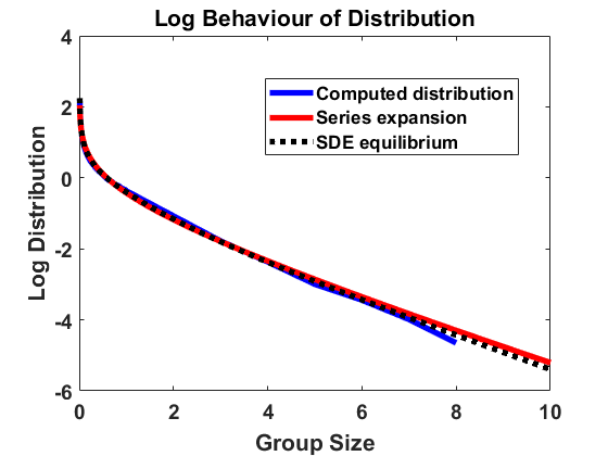 Figure 1
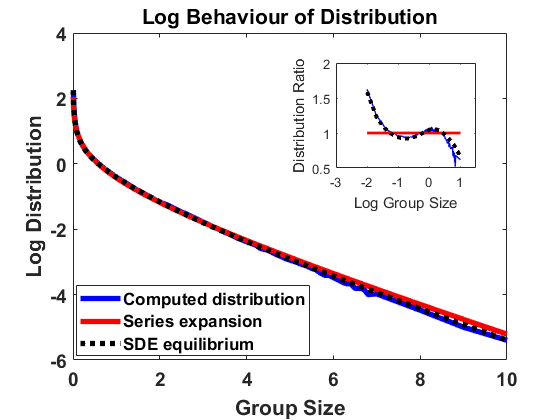 Figure 2
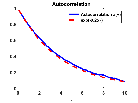 Figure 3
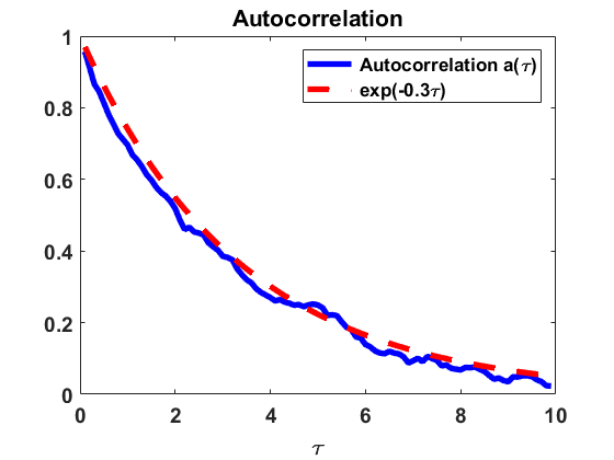 Figure 4
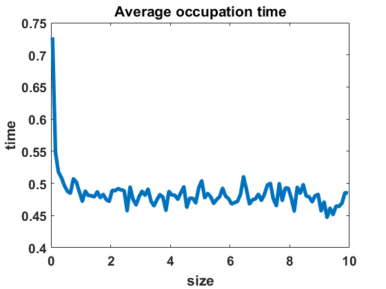 Figure 5
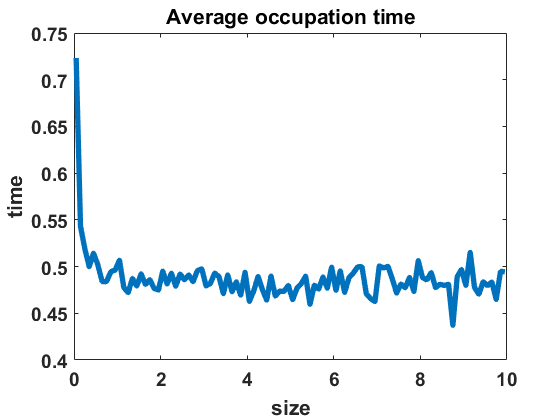 Figure 6
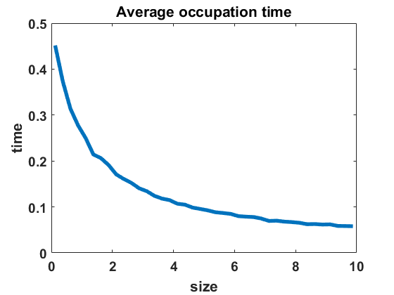 Figure 7
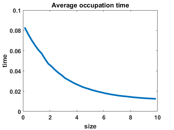 Figure 8
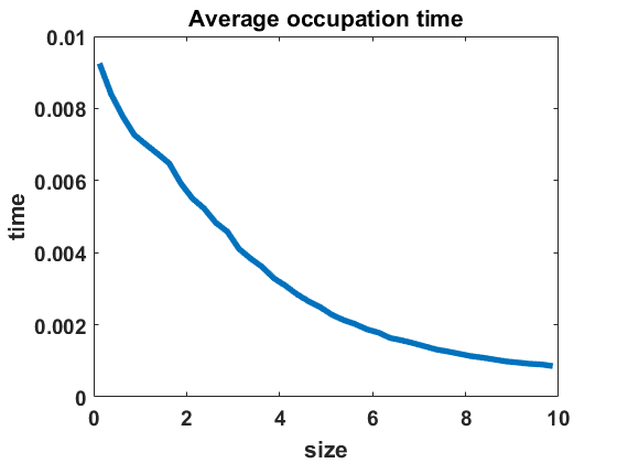 Figure 9
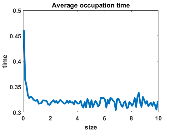 Figure 10
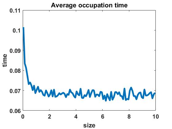 Figure 11
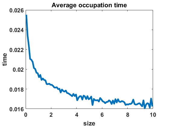 Figure 12
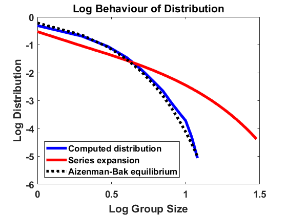 Figure 13
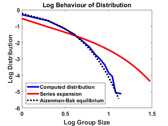 Figure 14
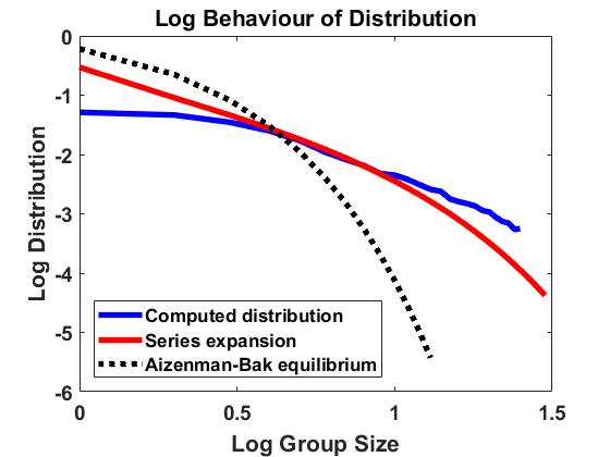 Figure 15
 Figure 16
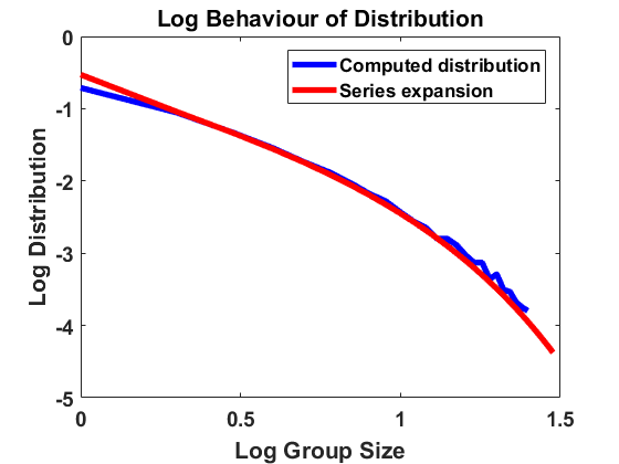 Figure 17
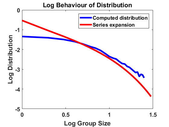 Figure 18
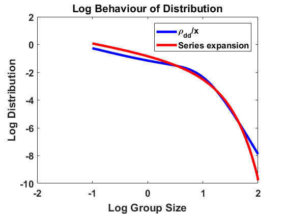 Figure 19
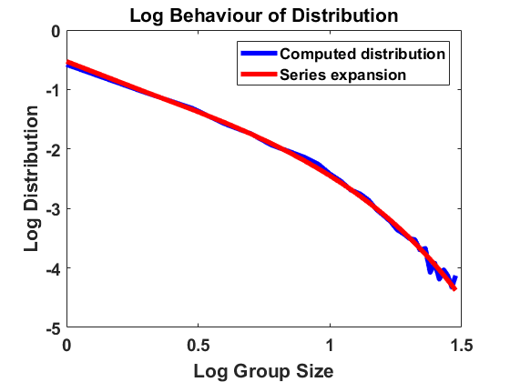 Figure 20
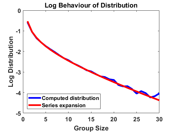 Figure 21
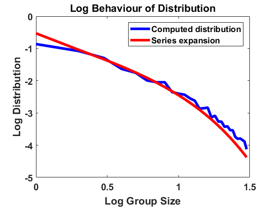 Figure 22
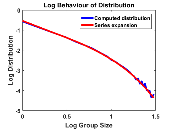 Figure 23
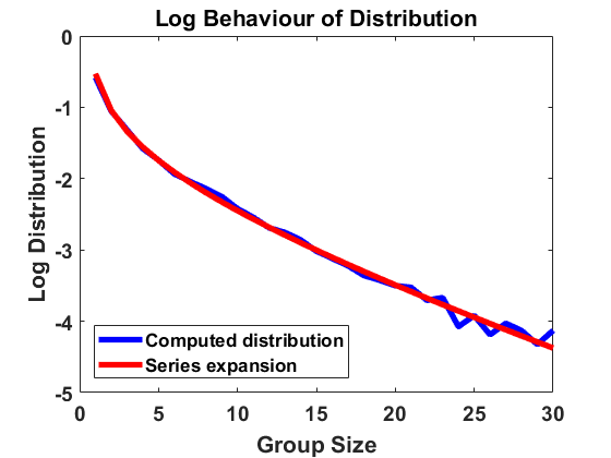 Figure 24
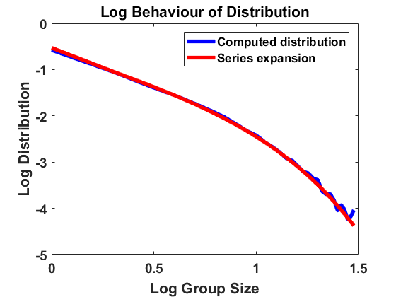 Figure 25
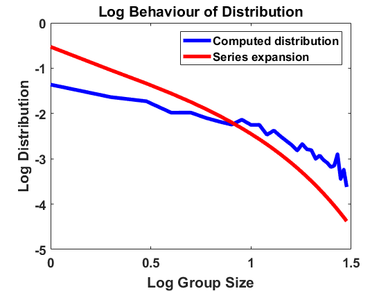 Figure 26
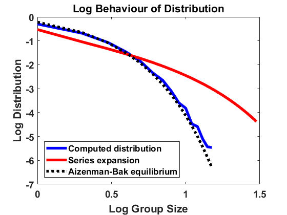 Figure 27
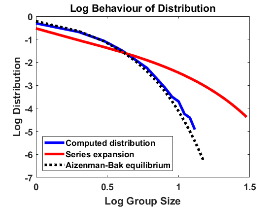 Figure 28
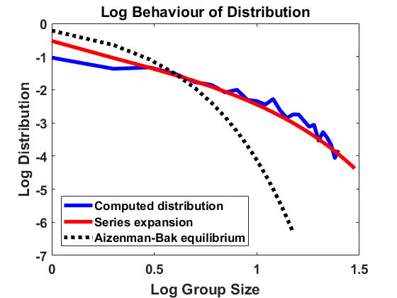 Figure 29
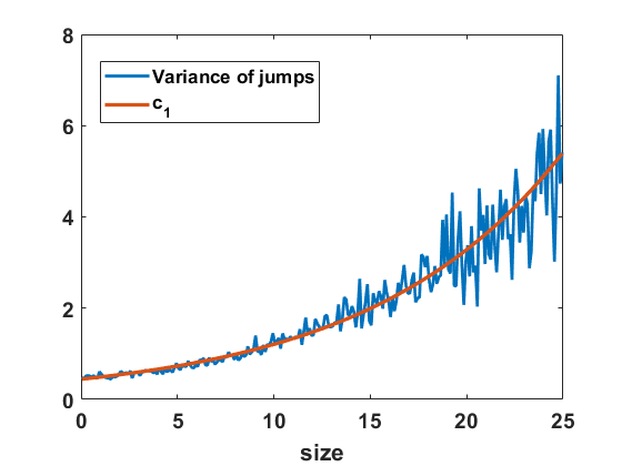 Figure 30
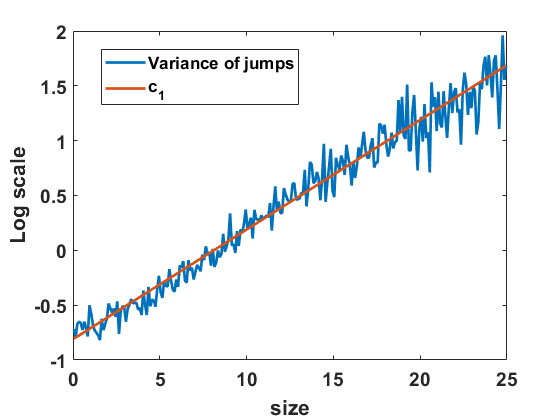 Figure 31
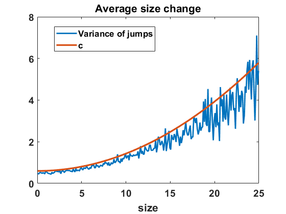 Figure 32
Peer Reviews
No public reviews on file for this paper yet. If you reviewed it on a platform where reviews are public (OpenReview, ICLR, NeurIPS, ICML), you can paste yours below so the community can read it here.
Videos
No videos yet. Explain this paper in a talk, walkthrough, or lecture? Add one.
Taxonomy
TopicsMathematical and Theoretical Epidemiology and Ecology Models · Mathematical Biology Tumor Growth · Evolution and Genetic Dynamics
A Markov jump process modelling animal group size statistics
Pierre Degond, Maximilian Engel, Jian-Guo Liu, Robert L. Pego Department of Mathematics, Imperial College London, London SW7 2AZ, United Kingdom. [email protected] of Mathematics, Technical University of Munich, Munich D-85748, Germany. [email protected] of Physics and Department of Mathematics, Duke University, Durham, NC 27708, USA. [email protected] of Mathematics, Carnegie Mellon University, Pittsburgh, Pennsylvania, PA 12513, USA. [email protected]
Abstract
We translate a coagulation-framentation model, describing the dynamics of animal group size distributions, into a model for the population distribution and associate the nonlinear evolution equation with a Markov jump process of a type introduced in classic work of H. McKean. In particular this formalizes a model suggested by H.-S. Niwa [J. Theo. Biol. 224 (2003)] with simple coagulation and fragmentation rates. Based on the jump process, we develop a numerical scheme that allows us to approximate the equilibrium for the Niwa model, validated by comparison to analytical results by Degond et al. [J. Nonlinear Sci. 27 (2017)], and study the population and size distributions for more complicated rates. Furthermore, the simulations are used to describe statistical properties of the underlying jump process. We additionally discuss the relation of the jump process to models expressed in stochastic differential equations and demonstrate that such a connection is justified in the case of nearest-neighbour interactions, as opposed to global interactions as in the Niwa model.
Keywords: Population dynamics, numerics, jump process, fish schools, self-consistent Markov process
Mathematics Subject Classification (2010): 60J75, 65C35, 70F45, 92D50, 45J05, 65C30
1 Introduction
The aggregation of animals into groups of different sizes involves a range of stimulating mathematical problems. On the one hand, the changes in size of the group a certain individual belongs to can be described, on the microscopic level, as a (stochastic) process. On the other hand, this process can be associated, on the macroscopic level, to the distribution of group sizes and the probability of individuals to belong to a group of a certain size (referred to below as the population distribution), and the evolution of such distributions in time. In particular, the existence and uniqueness of and convergence to an equilibrium distribution is a central object of interest.
Various models of describing the coagulation and fragmentation of groups of animals have been suggested and analysed in the past (cf. e.g. [3, 4, 17, 18, 32]). The model this work rests upon was introduced by Hiro-Sato Niwa in 2003 [29] related to studies in [27, 28, 30] and has turned out to hold for data from pelagic fish and mammalian herbivores in the wild. Niwa simulated a very simple merge and split process for a fixed population but he did not analyze the actual process he simulated. Instead, he used kinetic Monte-Carlo simulations to fit the noise in a stochastic differential equation (SDE) model for the size of the group that an individual animal belongs to. Due to its fairly simple form, he was able to find a closed formula for the stationary density of this SDE in a form similar to an exponential law (modified by a double-exponential factor), interpreting it as the equilibrium population distribution. Since the population distribution is related to the group-size distribution by a simple algebraic relation, he was able to find the equilibrium group-size distribution in a form close to an inverse power law with an exponential cutoff, namely
[TABLE]
In [29], Niwa showed that this expression provided a good fit to a large amount of empirical data with no fitting parameters.
In [7], we have pursued Niwa’s model based on a coagulation-fragmentation formulation for the distribution of group sizes and given a rigorous description of the equilibria for continuous and discrete cluster sizes. The lack of a detailed balanced condition presented a true mathematical challenge. However, by introducing the so-called Bernstein transformation, we have shown that there exists a unique equilibrium, under a suitable normalization condition, for both the discrete and the continuous cluster size cases. Furthermore, we provided numerical investigations of the model in [6].
In the present paper we develop Niwa’s original idea for modelling the population distribution through the group-size history of a fixed individual. We derive and study the naturally associated jump process rather than using the SDE framework, however. The jump process is described through a self-consistent Markovian approach as introduced in classic work of H. McKean [26], in which the rates of jumps for a (tagged) individual’s group size depend upon the (macroscopic) group-size distribution for the whole population. To be a self-consistent description of the dynamics, this macroscopic group-size distribution should coincide with the probability distribution that evolves under the jump process for the tagged individual.
This feedback makes it difficult to handle such a jump process analytically in the cases we wish to consider. (Some of the earliest analytic work on a general class of jump processes that follow McKean’s framework was carried out by Ueno [37] and Tanaka [35, 34]. A vast literature now exists on related McKean-Vlasov diffusion processes.) Therefore we develop an algorithm that approximates the jump process and which we can use to study the dynamics of the process and the equilibrium group-size distribution for variations of the Niwa model. The idea is to estimate the macroscopic group-size distribution for a large population of total size by the empirical distribution of a sample of tagged individuals with . This effectively results in a Markov jump process for the group sizes of a fixed number of tagged individuals, with transition rates driven by the population distribution of these individuals. A closely related time-continuous Markovian interacting particle system was studied by Eibeck and Wagner in [8] and [9] where they proved convergence of the empirical distribution to a solution of coagulation models which was extended to coagulation-fragmentation models, among others [10]. In this paper we will pay particular attention, however, not only to the estimated macroscopic group-size distribution, but to statistical and dynamical properties of the jump process for a tagged individual.
We refer to [2] for an early review of open problems relating Smoluchowski’s coagulation equations to stochastic models, including the standard Marcus-Lushnikov process [23, 21] for the size distribution of all groups in a fixed finite population. Our approach and the one in [9] deal with somewhat simpler jump-process models for the population distribution for a fixed number of groups (which can be regarded as those containing tagged individuals).
In [6], we approached the coagulation-fragmentation form of the Niwa model with three different numerical methods. One of them is a recursive algorithm derived from the discrete model in [22] which allows to compute the equilibrium precisely but only for fixed coagulation and fragmentation rates being constant over time and group sizes. It further does not give insight into the time-evolution. The second method is a Newton-like method which also only allows to approximate the equilibrium, but with the advantage of being adaptable to size-dependent merge and split rates. The third method is a time-dependent Euler method which is flexible towards arbitrary modifications of the model but numerically not efficient.
We will show in the current paper that our numerical scheme based on a Markov chain can be used to approximate the equilibrium for all different kinds of coagulation and fragmentation rates, allows for insights into the time evolution of the population distribution and also enables us to study properties of the process such as the statistics of occupation times in cluster sizes and the decay of correlations of trajectories. The method is accurate, efficient (in particular in equilibrium where it is sufficient to simulate only one trajectory), versatile, and gives insights into the dynamics on the individual level.
Furthermore, we will also discuss some shortcomings of Niwa’s SDE model for the temporal behavior of the size of the group containing a given individual. As merging and splitting occurs, involving interactions of groups of all different sizes, an individual’s group size can be expected to experience frequent large jumps. Yet the SDE model is an Ornstein-Uhlenbeck-type (OU-type) process that has continuous paths in time. One way this could be a reasonable approximation is if the jump process has mostly small jumps, for then there is a natural SDE approximation found through a second-order Taylor expansion. We find, though, that for the jump process in question, the equilibrium of the second-order SDE approximation is not consistent with the rigorously derived equilibrium in [7].
Another modeling issue is that the OU-type process will naturally produce unphysical (negative) group sizes. Some kind of reflection or symmetrization is needed to maintain positive sizes, but the natural choice leaves a free parameter in the model and is not motivated well by merging/splitting mechanisms. Niwa’s model also involves an exponentially growing variance which makes accurate numerical simulation difficult.
Lastly, we will point out that there is a kind of group-size dynamics, distinctly different from what Niwa simulated, that admits an SDE model whose equilibria are quite similar to the equilibria found in [29] and [7], but even simpler. The equilibria take exactly the form of a simple power law with exponential cutoff—a logarthimic or gamma distribution. This alternative SDE model for such distributions goes back to [24] and [33], and corresponds to a process with continuous sample paths guaranteed to stay in without hitting 0. We show formally the convergence of a nearest-neighbour model for jumps in group sizes to the equilibrium of this SDE.
The remainder of this paper is structured as follows. In Section 2, we derive the evolution equation of the population distribution for a coagulation-fragmentation model of size distributions, in general, and the Niwa model, in particular. Furthermore, this nonlinear evolution equation is shown to coincide with the master equation for a Markov jump process whose jump rates are determined self-consistently by the population distribution itself. Section 3.1 introduces the numerical scheme which is then used in Section 4 to simulate the process for different choices of coagulation and fragmentation rates. We validate the method by observing fast and accurate approach of the (known) equilibrium for the Niwa model and further use the algorithm to generate the size distributions for random and polynomial rates. In Section 5, we use the numerical method to estimate the decay of correlations of the Niwa jump process and, additionally, describe the statistics of ocuupation times for different kinds of rates. Finally, Section 6 is dedicated to the role of stochastic differential equations in the context of the aggregation models.
2 Description of the (self-consistent) Markov jump process for the population distribution
2.1 Evolution equation for the population distribution
The continuous version of a coagulation-fragmentation equation, called also Smoluchowski equation, describes the evolution of the number density of continuous sizes at time . In weak form it reads, for all test functions :
[TABLE]
The coagulation rate and fragmentation rate are both nonnegative and symmetric. The coagulation and fragmentation reactions can be written schematically
[TABLE]
By a change of variables, (2.1) can be transformed into
[TABLE]
Note that by taking , one obtains the conservation of mass
[TABLE]
Starting from the group size distrbution satisfying equation (2.2), we introduce the population distribution
[TABLE]
From (2.3) we observe that
[TABLE]
is conserved and corresponds to the total number of individuals .
In Niwa’s model [29], the coagulation and fragmentation rates are constant. The setting of the model assumes different zones of space on which individuals move, where is conserved through time. At each time step every group, whose size is a natural number , moves towards a randomly selected site with equal probability. When - and -sized groups meet at the same site, they aggregate to a group of size . So the coagulation rate is independent from the group sizes and can be written as for any where is the fixed coagulation parameter. The fragmentation rate expresses the fact that at each time step each group with size splits with probability independent of , and that if it does split, it breaks into one of the pairs with sizes with equal probability. As the actually distinct pairs are counted twice in such an enumeration, one gets for all with : .
The formulation for continuous cluster sizes gives
[TABLE]
where and for and being the constants in Niwa’s model. In this case the group size distribution satisfies the following equation [7]
[TABLE]
In [7, Theorem 5.1], the existence of a unique scaling profile for the equilibrium of (2.6) is proven, where for all and is a completely monotone function (infinitely differentiable with derivatives that alternate in sign) with asymptotic power laws.
We derive the general strong form for the population density corresponding with model (2.1), presented in the following Proposition, and thereby in particular for the Niwa model, as stated in the subsequent Corollary.
Proposition 2.1**.**
In strong form the evolution equation of the population density at any time , corresponding with (2.1), is given by
[TABLE]
Proof.
By testing (2.2) against we obtain:
[TABLE]
We remark that
[TABLE]
and by symmetry under exchanges of and , the first integral becomes
[TABLE]
Noting that the change of variables leaves the second integral invariant, we can restrict the interval of integration in to the interval upon multiplying the result by . So, the second integral equals:
[TABLE]
The resulting equation is thus
[TABLE]
To derive the strong form for the first integral in (2.9) we only need to conduct a change of variables for the term involving , namely :
[TABLE]
For the second integral, again by symmetry between and , it is enough to observe that
[TABLE]
This finishes the proof. ∎
Note from the weak form (2.9) in the proof that the merge process is done with rate while the split process is done with rate . Due to its dependence on , the merge process is characterized by a nonlinear term which turns out to be a challenging feature of the following analysis. First note that we obtain the following equation for the Niwa model:
Corollary 2.2**.**
In strong form the evolution equation of the population density at any time , corresponding with (2.6), is given by
[TABLE]
Proof.
From (2.9) we infer immediately that
[TABLE]
Again, the claim follows by an easy calculation. ∎
In this case we notice that the merge process is done with rate while the split process is done with rate for every .
2.2 Derivation of stochastic process
The key point of our approach is to regard the evolution equations (2.7) and (2.10) as master equations for a stochastic process that can be simulated, if the population density is already known. This stochastic process is essentially of the type whose study was initiated in McKean’s seminal work [26].
2.2.1 Reformulation of deterministic dynamics
For that purpose, we rewrite the equations as follows.
Lemma 2.3**.**
The evolution law in strong form (2.7) can also be written as
[TABLE]
where
[TABLE]
are the coagulation and fragmentation factors. In particular, in the Niwa model these factors are
[TABLE]
Proof.
The coagulation part follows immediately from (2.7). For the fragmentation part, we observe by using the symmetry between and that
[TABLE]
The factors for the Niwa model follow immediately from (2.5). ∎
We can summarize these terms, using that from (2.4), into
[TABLE]
Here, is the rate of change from to anything else, and , have an analogous interpretation specified to fragmentation and coagulation respectively. Eq. (2.3) can then be written as
[TABLE]
where
[TABLE]
is the corresponding probability of change from to some fixed . Formula (2.15) recalls the classical form of the forward equation for an associated jump process, as for example outlined in [16, Section X.3] or [11, Chapter 4.2]. However, the transition rates here depend on the density itself, and this makes the equation nonlinear.
Observe that formulas (2.15) and thereby (2.3) are consistent with the assumption of mass conservation, easily derived as follows:
[TABLE]
In the Niwa model,
[TABLE]
where is the zeroth moment of the group size distribution . Hence, the rate is finite as long as . Generally, according to [7, Theorem 6.1], there exists a unique global in time solution to (2.6) in terms of finite non-negative measures on for any finite non-negative initial measure. In particular, the solution was proved to have a smooth density if the initial group-size distribution has a density that is completely monotone.
Proposition 2.4**.**
[7, Theorem 6.1]** In the Niwa model, i.e., with rates (2.14), equation (2.15) has a unique global (in time) solution such that is completely monotone, if is completely monotone with finite zeroth and first moments. In this case, the zeroth moment in (2.17) satisfies
[TABLE]
and remains bounded for all .
Further, we recall that in [7] the existence of a unique scaling profile for the equilibrium of (2.6), depending on , and , is proven. The profile is completely monotone, with exponential decay as , and as , so . Hence, in the case of the Niwa model (2.10) we immediately obtain an explicit formula for equilibrium solutions of (2.15) which we will use for our numerical studies later: for (to which all parameter choices can be reduced), we conclude from [7, Theorem 5.1] via (2.4) that the unique equilibrium profile satisfies
[TABLE]
where is a smooth function with
[TABLE]
For mass , the equilibrium density is given by
[TABLE]
For general coagulation and fragmentation rates, one has to be careful in order to make sure that is finite, either by restricting the class of admissible or by truncating the domain to some compact set .
2.2.2 Jump process
We introduce a jump process in the following way: Denote the set of probability densities on by
[TABLE]
Assume is Borel-measurable with for all . For every , , we define a probability measure by setting, for each Borel-measurable subset ,
[TABLE]
We assume that is uniformly bounded, and that and are continuous in for each and . Then, by classical results of Feller [13] (see also [16, section X.3]) there is a unique solution of the backward equation
[TABLE]
for the transition function of a Markov process. (For generalizations of Feller’s results without continuity, see [11, Lemma 4.7.2] and [12].) Given any initial distribution , there exists a corresponding Markov (jump) process with initial density and transition function (see [11, Theorem 4.1.1] and also [20, Theorem 8.4]). This process solves the (time-dependent) martingale problem associated to the family of generators given by
[TABLE]
for all measurable and bounded functions . Moreover, the law of is given by
[TABLE]
Due to the assumption that is bounded (see [13]), the transition function also satisfies the forward equation
[TABLE]
and consequently, integration against shows that the law of also satisfies the forward equation
[TABLE]
In the stationary case when is constant in time, the Markov process can be constructed in a standard way [11, Section 4.2], from a Markov chain corresponding to time-independent rates and transition probabilities from (2.20), and a sequence of independently and exponentially distributed random variables.
Remark 2.5**.**
Considering Proposition 2.4, if is taken to be any solution of the Niwa model corresponding with a completely monotone initial group-size distribution , the boundedness and continuity assumptions indeed hold, and the Markov process is well defined. For general coagulation-fragmentation rate kernels and , however, we do not address the technical issue of what hypotheses on the kernels and on the initial data are sufficient to ensure that the boundedness and continuity assumptions hold.
2.3 Self-consistency
In order to guarantee self-consistency of this construction, we need to verify that if the function that is used in the definition of and is additionally assumed to be a solution of (2.7) (and hence (2.15)), then the law of the process is given by
[TABLE]
That is, we need to show that is distributed according to for all .
Let denote the right-hand side of (2.25). Then, upon integrating (2.15) over and using the definitions (2.20), we find that
[TABLE]
We have that . Thus to infer for all we need the initial-value problem for the forward equation (2.24) to have a unique solution with the properties enjoyed by both and .
That the requisite uniqueness holds is ultimately a consequence of our assumption on the boundedness of the transition rates . This assumption ensures that the solution of (2.23) is a conservative transition function, by which we mean that for all and .
Proposition 2.6**.**
Let , and satisfy the hypotheses stated in the previous subsection. Assume is a solution of (2.7) and . Then is distributed according to for all .
Proof.
We recall that the proof that follows an iteration argument (see [13, Theorem 1]) which is also sketched in [16, Appendix to X.3] in the time-homogeneous case. (The same result is established without continuity conditions in [12, Theorem 4.3].) By repeating the proof after integration against , it follows that is the minimal non-negative solution of (2.24) with that yields a measure satisfying for each . By consequence, for all and all . Because is conservative, it follows . Hence, for all ,
[TABLE]
and from this it follows . ∎
Remark 2.7**.**
As illustrated by Feller in [13], with unbounded jump rates it is possible for the natural solution of the backward equation (2.21) to fail to conserve total probability. We remark that it would be interesting to investigate how this may be related to the phenomena of gelation and shattering in solutions of the general coagulation-fragmentation equation (2.1).
3 Approximation of the stochastic process by a numerical scheme
3.1 The algorithmic scheme used in this paper
We approximate the jump process defined in Section 2.2.2 in and out of equilibrium by the following numerical scheme. Recall that kernels depend on the probability density . Hence, if the process is not stationary, i.e. in equilibrium, we need to estimate at every time step of the numerical scheme. Assuming where can be computed or at least approximated, we can study the dynamics in equilibrium. We will make use of our knowledge of the equilibrium profile in the case of the Niwa model.
In the following we explain the algorithm for the case in which the initial distribution is not the equilibrium distribution, and therefore we have to estimate at every time . It will become clear how the algorithm is conducted for fixed .
At the beginning, we fix the following quantities:
- •
an initial distribution on an interval for some (large) ,
- •
the coagulation coefficient and fragmentation coefficient ,
- •
the total number of individuals, i.e. the mass ,
- •
the number of sample individuals/particles (not to confuse with the total mass),
- •
the time step size ,
- •
the bin size for a partition of the domain .
We simulate the jump process for the individuals by computing, for each time step , the entries of the vector where the entry equals the group size of the th individual. In other words, denotes the vector which contains all the obtained cluster sizes at time . The initial vector is chosen according to , for example a uniform distribution. We divide the interval into bins of length , denoted by .
At every time step , we proceed as follows:
We estimate the coagulation and fragmentation probabilities for the centres of the bins :
- •
We approximate the density by
[TABLE]
where is the number of entries of in .
- •
Now we calculate the following quantities for all bin centres :
[TABLE] 2. 2.
We decide for each entry of if a jump happens, and if yes, where the jump goes to, in the following way:
- •
For each , we determine the bin in which it is contained. Furthermore, we generate a random number from the uniform distribution on the unit interval.
- •
If , nothing happens and stays in the same bin. Otherwise a jump happens.
- •
If a jump happens, we generate another random number from the uniform distribution:
- –
If , coagulation happens:
in this case we generate another random number from the uniform distribution and calculate for the sum
[TABLE]
until . Then we set .
- –
If , fragmentation happens:
in this case we generate another random number from the uniform distribution and calculate the sum
[TABLE]
until . Then we set . 3. 3.
In this way, we obtain the vector , which contains all the cluster sizes corresponding with the individuals at time . For time , the procedure starts again with the first step.
Approximating the exponential distribution with time discretization step size , the algorithm induces a Markov chain, simulating trajectories of the jump process corresponding with the generators
[TABLE]
acting on the bounded and measurable functions . The process approximates the jump process from Section 2.2.2 with generator (2.22) for , and, for small enough, the simulations give accurate results, as we will demonstrate in Section 4.
Remark 3.1**.**
If we assume that the population distribution is in equilibrium and we can compute or at least approximate with high accuracy, we can use the algorithm above to simulate the jump process by simply replacing as in (3.1) by at each time step . In this case, it is also sufficient to only track one individual for analyzing typical paths; that means that the vector only has one entry. The approximated process is a Markov process, as indicated in subsection 2.2.2 above.
Remark 3.2**.**
Note that we could also adopt the domain for each step by considering for some , instead of . However, if is large enough, the effect of such a measure is vanishingly small due to the fast decay in our models and, therefore, not necessary to obtain an accurate scheme.
3.2 Comparison to scheme by Eibeck and Wagner
As mentioned in the Introduction, there is a long history of stochastic particle methods for coagulation (and fragmentation) equations. Since the nonlinearity is contained in the coagulation terms, works on pure coagulation equations are highly relevant for our class of equations. For pure coagulation, the standard stochastic model, often referred to as a Marcus-Lushnikov process [23, 21], describes a Markov jump process that models the coagulation of clusters of size and to form a single cluster of size with rate kernel . In quite a number of studies (to be brief, we mention only [19, 31, 10]), the empirical measure for the group-size distribution has been related directly to the coagulation part of the Smoluchowski equation (2.1), in the so-called hydrodynamic limit as the number of particles becomes large.
In work more closely related to the present study, Eibeck and Wagner [9] developed a different approximation scheme to study the following mass flow equation for and continuous and compactly supported:
[TABLE]
This is the weak form of (2.7) (cf. also (2.8)), which we have referred to as evolution equation of the population density, in the case of pure coagulation. A solution of (3.3) is required to be in the set of all continuous paths with values in the set of non-negative Borel measures, i.e. .
The solution of (3.3) is approximated by a jump process for the empirical measure of an interacting particle system, formalized as a càdlàg process with values in a subset of . This jump process models the interaction of clusters of size and to result in a pair of clusters having sizes and . In this way, the distribution of cluster sizes in the particle system is used to estimate particle coagulation rates that determine jump rates for a fixed number of particles, in a way similar to the algorithm described in the previous subsection.
In more detail, suppose that for some continuous function where is non-increasing. For , and fixed , they define the set of measures
[TABLE]
Defining the map
[TABLE]
they introduce the generator on continuous and bounded functions
[TABLE]
which is shown to correspond with a jump process . Introducing the set
[TABLE]
one can view as a càdlàg process on , i.e. .
Under these assumptions, Eibeck and Wagner [9] prove weak convergence of to the solution of (3.3) for , as , and in [10] they provide a similar result for the case where fragmentation is added. In the corresponding algorithm, the coagulation kernel is replaced by the majorant product kernel which leads to a simple computation of the exponentially distributed waiting time for the collision and an independent generation of collision partners (cf. also [8] for the use of majorant kernels). When the collision partners and have been chosen according to the probabilities
[TABLE]
the jump happens with acceptance probability
[TABLE]
and, in this case, is removed and, if , is added to the points of the empirical measure.
Note that the essential difference between our scheme and such a method concerns the fact that we simulate single trajectories of individuals jumping between groups of different sizes, while the Eibeck-Wagner algorithm simulates the evolution of the population distribution as a whole as represented by the empirical measure. We track individual trajectories on the state space and therefore we can analyze the statistical properties of such trajectories, as we will see in Section 5.
4 Numerical simulations
In the following, we are using the algorithm developed in Section 3.1 to simulate the population dynamics for the coagulation-fragmentation model (2.1), or (2.7) in terms of the population density, with coagulation rates and fragmentation rates . Firstly, we validate the algorithm by working in the Niwa model (constant rates, see (2.5)) where the simulation results can be compared to a known equilibrium distribution. Furthermore, we use the algorithm to study the equilibrium and convergence to equilibrium in the cases of random and polynomial rates which demonstrates the flexibilty of our numerical scheme as opposed to previous ones, see [6].
4.1 Constant coagulation and fragmentation rates
First we work with the Niwa model (2.6), or (2.10) in terms of the population density, and compare our computation with analytical results. We conduct the numerical scheme described in Section 3.1 until a certain time , determining as in (3.1). Using the definition of the population distribution (2.4), we can determine
[TABLE]
as an approximation of the size distribution and compare the results with the analytic predictions.
For doing so we choose total mass and . Recall from [7] that any other combination of parameters can be reduced to this case by rescaling. According to [7], the equilibrium size distribution for (2.6) can be expanded as a series in the following way:
[TABLE]
where denotes the gamma function. We denote the partial sums by
[TABLE]
4.1.1 Jump process out of equilibrium
We compute according to the algorithm introduced above for , , , bin size and sample individuals which are initially distributed according to the uniform distribution on . As for most simulations in the following, the mass is normalized to . In Figure 1, we have averaged over larger bin sizes in order to obtain a smoother picture and used linear interpolation to create a continuous plot. The figure compares the computed density according to the algorithm with the analytical approximation, using (4.2). We show the results on a log-log and a semi-log scale, where log denotes the decadic logarithm in the following, unless stated otherwise. We observe that the algorithm produces convergence to a distribution that approximates the analytical expansion very well. For larger sizes, there are small deviations from the equilibrium due to the extremely small number of observations in this part of the domain. Overall, the stochastic method can be seen to be highly accurate.
4.1.2 Jump process in equilibrium
The simulation in equilibrium works with the same algorithm as in Section 3.1 but replaces at each time step by the approximation of the equilibrium density , obtained from as given in (4.2), via (2.4), see Remark 3.1. In this situation, it is sufficient to approximate the Markov process by simulating the trajectory of a single individual, deploying a simple Monte-Carlo algorithm.
For , and bin size , we approximate the stationary population distribution by measuring time averages of a single trajectory on the interval according to the modified algorithm (Remark 3.1), and, in Figure 2, we compare the corresponding stationary size distribution with the analytical prediction given by . We again average over the larger bin size and show continuous plots. As in Figure 1, we show the results on a log-log and a semi-log scale and observe exactly the same as in Section 4.1.1. The method is highly accurate except for small deviations from the equilibrium for large group sizes due to the extremely small number of observations in this part of the domain. Hence, we observe that the numerical scheme for simulating the Markov jump process in equilibrium is consistent with the analytical results.
4.2 Non-constant coagulation and fragmentation rates
As opposed to the analysis in [7] and most numerical methods presented in [6], the jump process approach and the associated algorithm do not rely on constant coagulation and fragmentation rates and . Hence, we use the flexibility of the algorithm to investigate non-constant choices for and . Hereby, we test the sensitivity of the results to changes in the model. We observe that random rates produce a clearly different outcome if the variance is high. Similarly, the equilibrium corresponding with polynomial rates separates from the Niwa equilibrium with increasing order of the polynomials. Furthermore, we study random and polynomial variations of the Aizenman Bak model [1] where and are constant and the equilibrium size distribution satsifies the detailed balance condition
[TABLE]
4.2.1 Random rates
In this section, we consider the coagulation and fragmentation rates and in model (2.1), and thereby (2.3), to be time-dependent. Furthermore, for all and , under preservation of symmetry, they are assumed to be log-normally distributed -correlated random variables with mean or respectively and standard deviation . This means that for all , the rates are sampled according to
[TABLE]
and the correlations are given by
[TABLE]
and analogously for . If , the model coincides with the Niwa model (2.6).
Setting again and thereby , we compute according to the algorithm introduced in Section 3.1, now sampling and according to (4.3) independently for every bin and at every time step. For the simulations displayed in Figure 3, we have chosen bin size , sample individuals and time length , starting with a uniform distribution and comparing the results for different values of the standard deviation . We use the time step size for and for to account for possible higher jump rates. As before, we average over larger bin sizes , use linear interpolation to create a continuous plot and compare the computed distribution to the analytical approximation in a log-log scale.
For the results are almost identical to the ones before, showing almost perfect accordance with the analytical expansion. Hence, the equilibrium appears to be robust under small random fluctuations. However, for we already observe a small discrepancy and for a clear discrepancy to the model with constant rates. The fact that mass is typically shifted to larger sizes suggests that high random fluctuations favour in average coagulation over fragmentation, even though the fluctuations are equally distributed for both rates. Due to the time-dependent and thereby non-autonomous nature of the random rates, the size distribution cannot reach an equilibrium but a state one could describe as almost steady, characterized by small fluctuations around an expected distribution. Making sure such a state is reached here, we have compared the simulation results at , and at and observed almost identical behaviour of the size distribution.
Moreover, we consider random fluctuations around the Aizenman-Bak model [1]. This means that for all , the coagulation and fragmentation rates are distributed according to
[TABLE]
where the correlations are given as in (4.4). Analagously to before, the case coincides with the Aizenman-Bak model with and . Setting , the stationary size distribution is known to be a simple exponential distribution with parameter , i.e. the stationary density of the size distribution is given by
[TABLE]
We use the jump algorithm as before to approximate the equilibrium distribution and compare it to the equilibrium of the Niwa model according to the series expansion as well as the equilibrium density , as shown in Figure 4. First, we set to compare the distributions without random fluctuations. We observe that the higher fragmentation rates in the Aizenman-Bak model lead to a shift of mass to smaller group sizes for compared with and that the algorithm approximates very well. Furthermore, we choose and to observe that, for small noise, the curves are again similar to the case , whereas, for larger noise, the equilibrium for (4.5) loses mass in the range of small group sizes and gets closer to the equilibrium (4.1) for model (2.6). In both the Niwa and the Aizenman-Bak model we observe that random rates with large noise drive the size distributions away from the deterministic equilibrium in the direction of a uniform distribution.
4.2.2 Polynomial rates
Furthermore, we consider polynomial coagulation and fragmentation rates. In terms of the physical model describing the dynamics of animal group aggregation, it seems plausible that the fragmentation probability increases with the group size. In addition, larger groups should also have a larger probability to be the result of a coagulation process. The easiest way to implement this reasoning in terms of polynomial rates is given by
[TABLE]
where , such that for we obtain the Niwa model with . Inserting the rates from (4.6) into (2.13) gives
[TABLE]
We use the jump algorithm from Section 3.1 with rates (4.6) to approximate the equilibrium and compare the result to the equilibrium of the Niwa model, estimated by the series expansion. We set , choose and use time step size for and for to account for the higher jump rates. We observe in Figure 5 that with increasing the distribution separates from the equilibrium profile with constant rates. While for the computed distribution coincides with and for the computed distribution is still very close to , we note that for the group sizes are closer to a uniform distribution. Similarly to the situation with random rates, we have compared the simulation results at and at and observed the same behaviour of the size distribution, making sure that the stronger vicinity to the uniform distribution is not caused by a slower convergence process.
The finding that increasing imply a divergence from the equilibrium profile with constant rates towards a uniform distribution can be accounted for by the fact that the rate of coagulation to large sizes increases with . This effect is apparently disproportionate to the impact of an increased rate of fragmentation from large sizes for increasing .
Similarly to the previous section, we additionally consider the coagulation and fragmentation rates
[TABLE]
where . In this case, the situation for coincides with the Aizenman-Bak model [1] where .
As before, for , we use the jump algorithm to simulate the dynamics with rates (4.7) and approximate the stationary density which we compare to the equilibrium of the Aizenman-Bak model and the equilibrium of the Niwa model. Recall from Figure 4 that the higher fragmentation rates in the Aizenman-Bak model lead to a shift of mass to smaller group sizes, compared with the Niwa equilibrium. We choose the same parameter values as for Figure 5 and observe in Figure 6 that, similarly to the model with rates (4.6) as shown in Figure 5, the equilibrium distribution seems to be driven away towards a uniform distribution under sufficiently increased exponents . Similarly to random rates with large variance, the increased coagulation and fragmentation probabilities of large sizes apparently tend to balancing each other out as opposed to the case with constant rates.
5 Statistical analysis of the jump process
The stochastic algorithm introduced in Section 3.1 can be used to study statistical properties of the jump process from Section 2.2.2. In the following, we estimate the decay of correlations for the process in equilibrium and starting out of equilibrium. Furthermore, we approximate the typical occupation times of individuals at cluster sizes for the different types of coagulation and fragmentation rates used in the previous chapter.
5.1 Autocorrelation function
The autocorrelation function gives an essential characterization of a stochastic process , by measuring the amount of memory the process keeps over times . In more detail, let denote the expected value and denote the variance of the process at time . Then the autocorrelation function is given by
[TABLE]
Fixing a time , we define the autocorrelation function in one time variable by
[TABLE]
We investigate numerically the autocorrelation function of the process , as in Section 2.2.2, for the Niwa model (2.10) with coagulation and fragmentation parameters , i.e. . We use the jump algorithm described in Section 3.1 to make a numerical estimate on the behaviour of , given that (a) the stationary density is reached, i.e. (see Remark 3.1), and (b) the equilibrium density is not reached yet but starting from a uniform distribution . In Fig. 7, we observe a rapid decrease of the autocorrelation , i.e. fast decay of correlations, in both cases. The findings suggest an exponential decay of correlations with a rate close to in equilibrium and a rate close to starting from a uniform distribution.
The numerical results indicate that, in the Niwa model, the size of the group an individual belongs to at a certain point of time is correlated significantly only to the sizes of the groups the individual belonged to in the close past. This is consistent with the underlying assumption that groups of all sizes can be involved in particular coagulations and fragmentations with equal probability.
5.2 Statistics of the occupation time
The second numerical investigation of the process’ statistical properties concerns the time individuals spend in average at a given cluster size before performing a jump to a new cluster size. We call this time length the average occupation time of each group size. We approximate this magnitude by conducting the algorithm from Section 3.1 with the four different types of coagulation and fragmentation rates, presented in Section 4: constant rates (), as in the original Niwa model, in equilibrium (Figure 8 (a)) and out of equilibrium (Figure 8 (b)), random rates as given in (4.3) (Figure 9 (a)-(c)) and polynomial rates as in (4.6) (Figure 9 (d)-(f)). For the random rates we compare and for the polynomial rates .
In Figure 8 and Figure 9, we display the approximated occupation times, averaging over bin sizes , for different choices of coagulation and fragmentation rates. We observe that the occupation times roughly reflect the corresponding equilibrium size distributions (or almost steady size distributions in the random case respectively), as seen in Section 4. In the case of coagulation and fragmentation rates (2.5) from the Niwa model, as shown in Figure 8, the occupation times show a sharp increase for smaller group sizes. We observe similar behaviour for small perturbations of the model, represented by the random case with (Figure 9 (a)) and the polynomial case with (Figure 9 (d)). Note that for random rates with and constant rates in equilibrium and out of equilibrium, the decay of occupation times stops at small sizes such that the occupation times fluctuate around a constant level for all larger sizes. In the case of polynomial rates, we observe smooth decay of occupation times mirroring the group size distribution in equilibrium more accurately.
The larger the random or polynomial perturbations of the Niwa model become, the more we see the peak at smaller sizes vanish. In fact, the average occupation times can be seen to decrease to a much smaller scale for increasing standard deviation in the case of random rates (Figure 9 (a)-(c)) and increasing polynomial exponents in the situation of polynomial rates (Figure 9 (d)-(f)), which can be explained by the increased coagulation and fragmentation rates and, thereby, increased jump rates. The decrease of occupation times to a similarly low level for all sizes is in accordance with the equilibrium density tending to a more uniform distribution for increasing random rates and increasing polynomial exponents, as seen in Figures 3 and 5.
6 SDE approximation to the jump-process model
Motivated by Niwa’s approach to use a stochastic differential equation (SDE) for modeling the dynamics and equilibrium distribution of group sizes [29], we discuss the role of SDEs for modeling the merging-splitting dynamics that correspond to the coagulation-fragmentation equation (2.1) or (2.7). First, we discuss Niwa’s SDE model and describe some of its problematic aspects. Next we derive a natural diffusion approximation to the group-size jump process of section 2.2, and demonstrate the inconsistency of this approach for modeling the jump process. Finally, we discuss an alternative SDE model for the dynamics of group sizes — a stochastic logistic equation — which, although it involves very different mechanisms for group-size changes, yields equilibrium group-size distributions that also have the form of a power-law with an exponential cutoff (gamma distribution).
6.1 Niwa’s SDE model
In order to find an expression for the equilibrium group-size distribution, Niwa [29] models the process of the size of the group containing a given individual via an SDE having the form
[TABLE]
when , where the parameter is related to the rate of group splitting per time step, the constant represents the population-weighted mean group size, and denotes standard Brownian motion. The drift is chosen linearly around the average, which roughly models the notion that, on average, fragmentation decreases group size by half, while coagulation increases it by a constant. Niwa modeled the noise coefficient using data from site-based merging-splitting simulations, coming to the conclusion that
[TABLE]
where is a constant. Ultimately though, there is no rigorous, or even formal, derivation of (6.1).
The stationary Fokker-Planck equation associated with the SDE (6.1) states that where is the probability flux
[TABLE]
Taking to ensure there is no flux at , one can solve this equation to find that the equilibrium population distribution takes the form
[TABLE]
where is a normalization constant. Correspondingly, the stationary group-size distribution is given as
[TABLE]
One problem in using (6.1) to model group-size evolution is that the process will hit [math], and one needs to specify how group size will be kept positive. Niwa appears to model this using symmetrization after a change of variables, and is led to impose the condition
[TABLE]
corresponding to (apparently in order to make a symmetrized drift potential continuously differentiable at 0). It seems more natural mathematically, instead, to simply require the stochastic process to reflect at 0. As described in [25, 36], e.g., this means that a term is added to the right-hand side of (6.1), where is the local time of the process at 0, determined by the formula
[TABLE]
The equilibrium density of this reflected process still has the form in (6.4) with , with normalization constant simply chosen to make a probability density on .
This leaves as a free parameter in the model, which one ought to specify in some further way. In terms of the quality of fitting (6.5) to the empirical data shown in [29, Fig. 5], it does not matter much what the precise value of is, as long as it is small. On the scale of [29, Fig. 5], the value provides a very acceptable fit, as was mentioned by Niwa himself [22] and was shown in [7, Fig. 2]. The simulation data Niwa generated in [29, Fig. 2] seem to be consistent with a much larger value of , however, that would not lead to a good fit with the data of [29, Fig. 5].
Since the stationary distribution (6.5) reasonably fits empirical data, one can consider whether the SDE (6.1) is a suitable basis for numerical simulation of the individual group-size process. We perform simulations using a simple Monte-Carlo scheme for an Euler-Maruyama integration of (6.1) with reflection and with step size , taking and imposing (6.6). (This means that the corresponding with , has to be rescaled as , see [7, Remark 5.1].) Following one trajectory up to time length , we approximate the stationary size distribution (6.5) on . In Fig. 10(a), we compare the result of the simulation, the density (6.5) and the rigorously derived equilibrium with , , estimated by the rescaled expansion . We observe that for small group sizes the approximation is relatively close to the other two densities, but for larger group sizes trajectories are lost although the time step size is already extremely small. This has to do with the highly unstable diffusion coefficient which is an exponential function. We actually can’t compute the distribution for sizes due to the unstable diffusion coefficient.
In order to avoid the exponentially unstable diffusion coefficient, we apply the following change of variables. Recall we take , . Similarly to Niwa [29], for we introduce by
[TABLE]
We formally use Itô’s formula to obtain, for ,
[TABLE]
Again we require the process to be reflected at 0, so this equation should be modified by a local time term. The strong negative drift near 1 prevents the exact process from hitting 1 (as one can check using the criterion from [15, Theorem 3], see Section 6.3.1 below). In a Monte-Carlo simulation, however, we have to prevent trajectories from leaving the domain at 1, by simply letting them stay at the same position in case the absolute value would become larger than . This Monte-Carlo algorithm, based on (6.9), yields Fig. 10 (b), where again the result of the simulation (with , ) is compared to the stationary density (6.5) and the rigorously derived equilibrium with , , estimated by the rescaled expansion . We observe that the distribution obtained by the simulation lies close to both densities but does not coincide with either of them which can be seen in particular for larger sizes.
Summarizing, modeling the dynamics via (6.1) or (6.9) lacks rigorous justification. The uniformly elliptic noise pushes the process to hit the origin and one must invoke ad hoc a means to keep it positive, unjustified in terms of the underlying population dynamics as originally outlined by Niwa.
Even though the simulated processes seem to reach an equilibrium close to the analytical prediction (see Figure 10), another serious modeling issue is that SDE sample paths are always continuous in time, and do not make large jumps in the way the merging/splitting mechanism would suggest. It is not clear whether the solution process of such an SDE can be related to the Markov jump process which is derived in Section 2.2 and simulated successfully in Section 4. The next section explores the possibility of such a connection.
6.2 SDE and the jump process
In the following, we investigate the suitability of a natural drift-diffusion approximation to the jump process constructed in Section 2.2.2, in the situation of the Niwa model with coagulation and fragmentation factors (2.5). Recall from (2.22) the family of generators
[TABLE]
where and are given by (2.20). Writing, similarly to before, , the forward equation for the jump process is the Fokker-Planck equation
[TABLE]
as given in (2.15). Matching [7], as before, we take and and assume that we are in equilibrium, i.e. for all , such that , and are time-independent. In equilibrium, we observe that
[TABLE]
Using the moment relations in [7, Eq. (5.6)] yields
[TABLE]
where . This means constant event rates, which is consistent with the fact that the system is in equilibrium. We obtain
[TABLE]
Now, supposing that the jumps go typically to a close range of sizes, we use the Taylor approximation
[TABLE]
to get , where the drift-diffusion approximation to the jump-process generator is given by
[TABLE]
with
[TABLE]
Note that represents the drift and the diffusion coefficient. We can conclude from (6.10) that in equilibrium these coefficients are as follows: using , the drift is given as
[TABLE]
Note that the signs are consistent with the model since the drift pushes to the right at small and the left at large , as expected. Using that from [7, Eq. (5.6)], the diffusion coefficient reads
[TABLE]
For the SDE with drift and diffusion , the Fokker-Planck equation corresponding with (6.11) is
[TABLE]
The stationary solution of this equation satisfies
[TABLE]
After integration, we can determine
[TABLE]
The stationary density for the approximating SDE with generator (6.11) differs rather substantially from the stationary solution of (2.10) for , which is given by (2.18). See the comparison of group size distributions in Figure 11(a), and note that each tick mark on the vertical scale corresponds to 2 orders of magnitude. For small group size, we have const, while from (2.18). Furthermore, while decays exponentially, decays only algebraically fast with as . One trouble is that for large sizes, the drift and diffusion rates are dominated by the (uniform) fragmentation mechanism, which is not well-described by small jumps.
Recall that Niwa estimates the diffusion coefficient for the SDE (6.1) by fitting it into a semi-log plot of the variance of size changes in finite time intervals, based on data obtained from site-based simulations of merging and splitting [29, Figure 2]. We can deploy the algorithm for the Markov jump process in equilibrium to approximate the variance of size changes and compare the computations to the diffusion coefficient . In Figure 11(b) we observe that size changes exhibited by the simulated jump process differ noticeably from the function (scaled by as appropriate), but not by a large percentage. By fitting on a semi-log scale as indicated in Figure 12(a) we find a good fit with a similar exponential form as Niwa had, namely with
[TABLE]
6.3 Model with degenerate noise
So far, we have ascertained that the adequate stochastic method for studying the coagulation-fragmentation model (2.1) with non-local rates in general and the Niwa model (2.6) in particular is given by a jump process, as derived in Section 2.2. Finding a stochastic differential equation whose solution is closely related to the underlying jump process has turned out to be analytically (Section 6.2) and numerically (Section 6.1) cumbersome. However, one can still try to find an SDE which models coagulation and fragmentation dynamics differently and displays the same or a similar equilibrium distribution as the evolution equation (2.15). In the following, we consider a stochastic logistic equation and its relation to a nearest-neighbour random walk.
6.3.1 Stochastic logistic equation and gamma distribution
From data plotted in [7, Figure 2] and [22], one can see that both the equilibrium profile (4.1) for the coagulation and fragmentation model (2.6) and the equilibrium profile (6.5) for Niwa’s SDE (6.1) model with and are close to the simple logarithmic size distribution profile
[TABLE]
in the range containing most of the empirical data plotted in [29, Figure 5]. Hence, we can also try to find an SDE, derived from a coagulation-fragmentation model for particles, such that the population distribution
[TABLE]
is the stationary solution of the corresponding Fokker-Planck equation. Pursuing this objective, we consider the stochastic logistic equation
[TABLE]
as suggested by Robert May in [24], and studied in [33]. If an invariant distribution exists, its density is the solution of the stationary Fokker-Planck equation
[TABLE]
The density must take exactly the form of a power law with exponential cutoff — a gamma distribution,
[TABLE]
When , is integrable on and is exactly the normalization constant. Note that we recover the exponential distribution (6.16) by choosing , and . When , no invariant distribution exists — instead one expects the process to spread out indefinitely as in the case when .
In equation (6.17), the degenerate diffusivity proportional to prevents the stochastic process from hitting [math] — this is a well-known phenomenon orginating with work of Feller [14]. In particular, the criterion of Theorem 3 of [15] states that the solution of (6.17) can hit [math] if and only if for all , all solutions of the ODE
[TABLE]
on are bounded in a neighborhood of [math]. To determine whether this is the case, one can change variables via and note that the theory of asymptotic behavior of ODEs [5, Section 3.8] allows us to neglect the term in the limit . Since the equation
[TABLE]
has unbounded solutions, we conclude that the solution process for (6.17) naturally stays in and no further assumption needs to be made about what happens at 0.
We note that the degenerate nature of the diffusion does neither reflect Niwa’s simulation results, which he used to estimate diffusivity for the SDE model (6.1) of the merging-splitting dynamics [29, Figure 2], nor the diffusion coefficient (6.2) for the second order approximation of the jump process. Recall that neither of these approaches delivered results that justifiably model the merging-splitting dynamics described by the jump process. In contrast, the logistic SDE model (6.17) consistently describes group-size fluctuations that occur due to a different mechanism, namely a geometric Brownian motion with logistic drift. Consequently, (6.17) is capable of providing a rationale for the appearance of the gamma distribution if the group-size dynamics are governed by a suitable mechanism.
In order to understand better what kind of mechanism could lead to (6.17), we note that some basic features observed in merging-splitting dynamics resemble principles expressed in (6.17): The linear multiplicative noise term can be interpreted to correspond with fluctuations increasing with the cluster size due to an increase in “coagulation and fragmentation interactions”. The logistic drift term expresses the dominance of fragmentation for larger sizes and dominance of coagulation for smaller sizes. In the following, we make these notions more precise by describing how a classical nearest-neighbor random walk on the lattice (corresponding to small jumps in group size among a discrete set) formally corresponds in the continuum limit to the stochastic logistic SDE model (6.17).
6.3.2 A lattice random walk approximating the stochastic logistic model
Consider a stochastic process determined exclusively by jumps to the nearest neighbours on the lattice with small grid size on . We let denote the probability of an individual to be in a group of size at time , and suppose that the group size can change only by jumps from to . We let denote the rate of jumps from to and let denote the rate of jumps from to .
The master equation for the corresponding process on the lattice is
[TABLE]
We exclude the origin by setting and will ignore the boundary henceforth. We can rewrite equation (6.21) as
[TABLE]
where
[TABLE]
is the flux from to , and, hence,
[TABLE]
is the flux from to .
Let us consider how to choose and to approximate a given SDE
[TABLE]
on . Recall that in the case of (6.17) we have
[TABLE]
The Fokker-Planck equation associated with the SDE (6.23) is
[TABLE]
Deploying a key idea from numerical analysis, we write the modified drift as the difference of positive quantities
[TABLE]
For our example (6.24) we can take
[TABLE]
Now we discretize the Fokker-Planck equation (6.25), using upwinding for the drift:
[TABLE]
This equation takes the conservative form in (6.22) with jumping rates
[TABLE]
In the case of the stochastic logistic equation (6.17), with drift and diffusion coefficients given by (6.24), we take and , , . Hence, we have
[TABLE]
The jump rates and both consist of a term with factor , corresponding with the drift in (6.17), and a term with factor , corresponding with the diffusion in (6.17). The terms with factor are all quadratic in the discrete size , as one would expect. The -term in is linear in and has a stronger relative impact on jumps to the right the smaller is, as in (6.17). In the rate the -term is quadratic in , as in (6.17), implying that both terms contribute to the increasing rate of jumps to the left in the same way. This gives a particular lattice random walk which approximates model (6.17) for small .
Note that a probability density satisfying for all the ratio
[TABLE]
is an equilibrium for (6.22). We check this condition for where is the gamma distribution from (6.19). First, we observe with a first order Taylor expansion at that
[TABLE]
On the other hand, we expand at to obtain
[TABLE]
Recall that choosing and in (6.17) gives the exponential population distribution (6.16). In this case we obtain and
[TABLE]
Observe that for any given the discrete size grows proportionally as is taken smaller. Therefore, the equilibrium ratio relation (6.27) is satisfied at in the continuum limit for (6.28), i.e. when and .
This formal derivation indicates that, in terms of the equilibrium density , the SDE model (6.17) with suitable parameters approximates the nearest neighbour model with jump rates (6.26). Hence, modelling the coagulation-fragmentation dynamics by the stochastic logistic equation (6.17) appears coherent with an underlying locally restricted jump process. This scenario avoids the main problem of the SDE modelling discussed in Sections 6.1 and 6.2 where the global aspect of the jump dynamics associated with (2.3) cannot be captured by the continuous solution of a stochastic differential equation.
7 Conclusion
For coagulation-fragmentation models of the form (2.1), we have derived the evolution equation (2.7) for the population distribution and a formalization of the underlying jump process. The associated algorithm has been validated by showing its accordance with the equilibrium for (2.6) and its versatility has been demonstrated by also working with different coagulation and fragmentation rates and a numerical study of the respective statistical properties.
Compared to the numerical methods for simulating Niwa-like coagulation and fragmentation models developed and summarised in [6], the jump process algorithm has been shown to be the most versatile and dynamically insightful scheme, by tracking the behaviour of individual trajectories. We have seen that, in particular, the rates can be chosen to be random or polynomial. This opens new, potentially more realistic, modelling possibilities that can be further investigated in future work.
Although Niwa’s SDE is neither rigorously justified nor particularly well-suited for numerical investigations, it has proven to be an insightful approach to the problem at hand. In Section 6.2 we have mathematically derived an alternative drift-diffusion approximation to the jump process whose equilibrium distribution shows similar behavior as the equilibrium for the jump process but does not coincide. To overcome the inherent discrepancy between continuous solutions of SDEs and processes with large jumps, we have indicated an additional possibility using an SDE with degenerate noise (stochastic logistic model) whose equilibria exactly take the form of gamma distributions and which can be related to a nearest-neighbour jump model. A more thorough investigation of that matter is left for future work.
Another future line of investigation could lead to spatialized models where coagulation and fragmentation rates depend on the location of the groups in space. One could imagine several types of spatial inhomogeneties, for example caused by attracting regions with high coagulation activity or volatile regions with high fragmentation probabilities. Such models would have a more direct correspondence with population dynamics and would give rise to new challenges that could be tackled by a jump process approach as discussed in this paper.
Acknowledgments
PD acknowledges support by the Engineering and Physical Sciences Research Council (EPSRC) under grant no. EP/M006883/1 and EP/P013651/1, by the Royal Society and the Wolfson Foundation through a Royal Society Wolfson Research Merit Award no. WM130048 and by the National Science Foundation (NSF) under grant no. RNMS11-07444 (KI-Net). PD is on leave from CNRS, Institut de Mathématiques de Toulouse, France. M.E. gratefully acknowledges support from the Department of Mathematics, Imperial College London through a Roth Scholarship and by the German Research Foundation (DFG) via grant SFB/TR109 Discretization in Geometry and Dynamics. This material is based upon work supported by the National Science Foundation under grants DMS 1812573 (JGL) and DMS 1812609 (RLP) and by the Center for Nonlinear Analysis (CNA) under National Science Foundation PIRE Grant no. OISE-0967140, and by the NSF Research Network Grant no. RNMS11-07444 (KI-Net).
Data statement
No new data were collected in the course of this research.
The reference list from the paper itself. Each links out to its DOI / PubMed record.
- 1[1] M. Aizenman and T. A. Bak. Convergence to equilibrium in a system of reacting polymers. Comm. Math. Phys. , 65(3):203–230, 1979.
- 2[2] D. J. Aldous. Deterministic and stochastic models for coalescence (aggregation and coagulation): a review of the mean-field theory for probabilists. Bernoulli , 5(1):3–48, 1999.
- 3[3] E. Bonabeau and L. Dagorn. Possible universality in the size distribution of fish schools. Phys. Rev. E , 51:5220–5223, 1995.
- 4[4] E. Bonabeau, L. Dagorn, and P. Freon. Scaling in animal group-size distributions. Proc. Natl. Acad. Sci. USA , 96:4472–4477, 1999.
- 5[5] E. A. Coddington and N. Levinson. Theory of ordinary differential equations . Mc Graw-Hill Book Company, Inc., New York-Toronto-London, 1955.
- 6[6] P. Degond and M. Engel. Numerical approximation of a coagulation-fragmentation model for animal group size statistics. Netw. Heterog. Media , 12(2):217–243, 2017.
- 7[7] P. Degond, J.-G. Liu, and R. L. Pego. Coagulation-fragmentation model for animal group-size statistics. J. Nonlinear Sci. , 27(2):379–424, 2017.
- 8[8] A. Eibeck and W. Wagner. An efficient stochastic algorithm for studying coagulation dynamics and gelation phenomena. SIAM J. Sci. Comput. , 22(3):802–821, 2000.