This paper investigates the behavior of the multiplication map over quotient rings of residually finite Dedekind domains, providing a detailed description of its dynamics and exploring various applications.
Contribution
It offers a novel analysis of the dynamics of the $a$-map over these algebraic structures, extending previous work to a broader class of rings.
Findings
01
Characterization of the $a$-map dynamics over quotient rings
02
Identification of structural properties influencing the map's behavior
03
Applications demonstrating the utility of the main results
Abstract
Let D be a residually finite Dedekind domain, a∈D be a nonzero element and n be a nonzero ideal of D. In this paper we describe the dynamics of the map x↦ax over the quotient ring D/n. We further present some applications of our main result.
No public reviews on file for this paper yet. If you reviewed it on a platform where reviews are public (OpenReview, ICLR, NeurIPS, ICML), you can paste yours below so the community can read it here.
Videos
No videos yet. Explain this paper in a talk, walkthrough, or lecture? Add one.
Taxonomy
TopicsCoding theory and cryptography · Algebraic Geometry and Number Theory · Finite Group Theory Research
Full text
Dynamics of the a-map over residually finite Dedekind Domains and applications
Universidade Estadual de Campinas, Instituto de Matemática, Estatística e Computação Científica, Campinas, SP 13083-859, Brazil.
Universidade de São Paulo, Instituto de Ciências Matemáticas e de Computação, São
Carlos, SP 13560-970, Brazil.
Abstract
Let D be a residually finite Dedekind domain, a∈D be a nonzero element and n be a nonzero ideal of D. In this paper we describe the dynamics of the map x↦ax over the quotient ring D/n. We further present some applications of our main result.
Finite dynamical systems associated with special types of functions have been extensively studied in the literature. For instance, iterations of quadratic polynomials over finite fields (motivated in part by some cryptographic applications such as the Pollard-rho factorization algorithm) were studied in [9, 13, 18]. Dynamic of Chebyshev polynomials of prime degree and its relation with decomposition of primes in certain towers of number fields were studied by A. Gassert in [1] and [2]. Dynamic of Chebyshev polynomials of arbitrary degree was studied in [11]. Dynamic of special types of linearized polynomials over finite fields was described in [8]. Dynamic of rational maps over finite fields such as Rédei functions [10] and maps of the form x↦k(x+x−1) [15, 16] have also been considered. The dynamic of certain maps associated with endomorphism of ordinary elliptic curves over finite fields was dealt in [17]. A survey on iteration of functions over finite fields is given in [4].
In this paper, we consider a residually finite Dedekind Domain, which we denote by D, a nonzero element a∈D, a nonzero ideal n⊴D and study the dynamic of the a-map Γa,n given by:
[TABLE]
where Ψn:D→D/n is the canonical epimorphism (i.e. Ψn(x)=x+n). We bring a unified frame to the study of several dynamical systems, some of them mentioned above, via the dynamic of the maps Γa,n. In general, the dynamic of a map f over a finite set X can be described through its associated functional graph G(f/X) whose vertices are the elements of X and (directed) edges of the form (x,f(x)) for x∈X. In dynamical systems, two maps f:X→X and g:Y→Y are called conjugates when there is a bijection h:X→Y such that h∘f=g∘h. In this case, h establishes an isomorphism between the functional graphs G(f/X) and G(g/Y). Our main result is a complete description of the functional graph G(Γa,n) up to isomorphism (Theorem 3.6). This result naturally extends the structural theorem for the functional graphs associated with the a-map over cyclic groups and with Rédei functions over finite fields given in [10], see also [12, Proposition 2.1]. Other corollary of our main result is a complete description of the functional graphs associated with linearized polynomials over finite fields, extending results given in [8]. These polynomials have many interesting properties and appear in diverse areas such as network coding theory [19] and finite projective geometries; see for example Chapter 3.4 of [3] and the notes at the end of this chapter for more properties and applications of these polynomials. The hanging trees attached to some periodic points of Chebyshev polynomials and maps induced by endomorphism of elliptic curves considered in [17], both over finite fields, can also be explained from our main result.
This paper is organized as follows. In Section 2 we cover some preliminaries results and fix some notation to be used throughout this paper. In Section 3 we prove our main result (Theorem 3.6) and provide a concrete example. In Section 4 we show several specializations of our main result; in particular we completely describe the dynamic of linearized polynomials over finite fields.
2 Preliminaries
In this section, we provide background material that is used along the way and some preliminary results heading to the proof of our main result.
2.1 On residually finite Dedekind Domains
Let D be a residually finite Dedekind Domain (i.e. D is an integral domain in which every nonzero proper ideal n factors into a product of prime ideals and the residue class ring D/n is finite). For ideals n and m of D, we denote m∣n if there is an ideal m′⊴D such that n=mm′. In a Dedekind domain, we have that m∣n if and only if n⊆m and consequently gcd(n,m)=n+m. When gcd(n,m) is principal, say gcd(n,m)=fD, we abuse of notation and write gcd(n,m)=f. For example, gcd(n,m)=1 means n+m=D and we say that n and m are relatively prime ideals. In this case we have n∩m=nm. The radical of an ideal n is defined as rad(n)={d∈D:di∈n\mboxforsomei∈Z+}. In a Dedekind domain rad(n) is the product of the distinct prime ideals factors of n. If a∈D is a nonzero element and n⊴D is a nonzero ideal we have a unique decomposition n=n0n1 where ⟨a⟩⊆rad(n0) and gcd(n1,⟨a⟩)=1; we refer to this decomposition as the a-decomposition of the ideal n.
The norm, Euler Phi function and multiplicative order for Dedekind domains are defined as follows.
Definition 2.1**.**
Let n be any nonzero ideal of D.
The normND(n) of n is the cardinality of the residual class ring D/n.
2. 2.
If n is a proper ideal of D, the Euler Phi function φD(n) of n is the cardinality of the group of units U(D/n) of D/n. If n=D, φD(n):=1.
3. 3.
For any element a∈D such that ⟨a⟩+n=D, let ord(a,n) be the least positive integer i such that ai−1∈n, or equivalently, ai≡1(modn).
It is well known that the norm ND is completely multiplicative, the Euler Phi function φD is multiplicative and, for any nonzero ideal n of D:
[TABLE]
where the product above is over all the distinct prime ideals dividing n; see for example [7, Chapter 1]. In particular, if p is any nonzero prime ideal of D and i is a positive integer, we have that
[TABLE]
We observe that, from definition, ⟨a⟩+n=D if and only if Ψn(a)∈U(D/n) and, in this case, ord(a,n) is the multiplicative order of Ψn(a). Then, by Lagrange theorem, ord(a,n)∣φD(n). The following result provides information on the existence and number of solutions of linear congruences in Dedekind domains.
Let D be a residually finite Dedekind Domain and n an ideal of D. For a,b∈D, the linear congruence
[TABLE]
is solvable if and only if b∈⟨a⟩+n. Furthermore, if the congruence is solvable, then it has exactly N(⟨a⟩+n) incongruent solutions modulo n.
Let p be any nonzero prime ideal of D and α≥1. For each nonzero element b∈D, we denote by νp(b) the exponent of p in the factorial decomposition of ⟨b⟩ into product of prime ideals. Since the ideals of D/n are exactly the ideals of the form Ψn(a) with a∣n, the quotient ring D/pα is a finite local ring. The following result has easy verification.
Lemma 2.3**.**
Let α≥1 and m be the maximal ideal of D/pα. The following statements hold:
m* is the homomorphic image of p by Ψpα and, in particular, m is principal;*
2. 2.
for any nonzero element b∈D such that Ψpα(b)=0, νp(b) is the only nonnegative integer i such that Ψpα(b)∈mi∖mi+1 (with the convention m0=D/pα);
3. 3.
for each 0≤i≤α, ∣mi∣=ND(pα−i).
From the previous lemma, we obtain the following result.
Lemma 2.4**.**
Let D be a residually finite Dedekind Domain and n∈D a nonzero ideal. For each ideal m dividing n, there exists φD(n/m) incongruent elements b∈D modulo n such that gcd(⟨b⟩,n)=m.
Proof.
If m=n, the result is trivial so we assume that m=n. Let k(m,n) be the number of incongruent elements b∈D modulo n such that gcd(⟨b⟩,n)=m. From the Chinese remainder theorem, k(m0,n0)⋅k(m1,n1)=k(m0m1,n0n1) whenever m0+m1=n0+n1=D. So we only need to consider the case that n=pα for some α≥1 and some (nonzero) prime ideal p of D and m=pi with 0≤i<α. However, in this case, we observe that a nonzero element b∈D is such that gcd(⟨b⟩,pα)=pi with 0≤i<α, if and only if νp(b)=i, i.e., Ψpα(b)∈mi∖mi+1. Therefore, k(pi)=∣mi∖mi+1∣=∣mi∣−∣mi+1∣ and so, from Lemma 2.3 and Eq.(2), we have that
[TABLE]
∎
2.2 Operations on functional graphs, elementary trees and ν-series
Most definitions and notations introduced here are taken from [10]. We denote
by ⨁i=1kGi the disjoint union of the graphs
G1,…,Gk and k×G=⨁i=1kG for k∈Z+. If m∈Z+ and T is a rooted tree, we denote by
Cyc(m,T) a graph with a unique directed cycle of length m, where
every node in this cycle is the root of a tree isomorphic to T. The tree T with a unique node is denoted by ∙. An extended rooted tree is a graph of the form Cyc(1,T) for some rooted tree T, in this case we write {T}=Cyc(1,T). A forest is a disjoint union of rooted trees and an extended forest is a disjoint union of rooted trees and extended rooted trees.
If G=⨁i=1kTi is a forest where T1,…,Tk are rooted trees, we denote by
⟨G⟩ a rooted tree verifying that its root has exactly k predecessors v1,…,vk where vi is the
root of a tree isomorphic to Ti for i=1,…,k.
To each non-increasing finite sequence of positive integers V=(ν1,ν2,…,νd) (i.e. ν1≥ν2≥⋯,νd≥1) we can associate a rooted tree TV defined recursively as follows:
[TABLE]
Trees associated with non-increasing sequences as above are called elementary trees; see Figure 1. We note that, by definition, if V=(ν1,…,νd) and W=(ν1,…,νd,1,1,…,1) then TV=TW.
Next we extend the definition of ν-series introduced in [10] to Dedekind domains.
Definition 2.5**.**
Let D be a Dedekind domain, a∈D be a nonzero element and n0⊴D be a nonzero ideal such that ⟨a⟩⊆rad(n0). The ν-series associated with n0 and a is the sequence of positive integers n0(a):=(N(a1),…,N(ad)) where N(a) denotes the norm of the ideal a and the ideals a1,…,ad are given as follows:
[TABLE]
where d is the least positive integer such that a1⋯ad=n0. When n0=⟨b⟩ is a principal ideal of D we denote b(a):=n0(a).
The next result is a direct consequence of the fact that gcd(qq′,n)=gcd(q,n)⋅gcd(q′,n) if gcd(q,q′)=1 and the definition of ν-series.
Lemma 2.6**.**
Let D be a Dedekind domain, a∈D be a nonzero element and q,q′ be nonzero ideals such that ⟨a⟩⊆rad(q), ⟨a⟩⊆rad(q′) and gcd(q,q′)=1. Suppose that q(a):=(N(a1),…,N(ad)) and q′(a):=(N(a1′),…,N(ad′′)) with d′≤d. Then, qq′(a):=(N(b1),…,N(bd)) with
[TABLE]
The tree Tn0(a) associated with the ν-series n0(a) plays an important role in the description of the functional graph G(Γa,n).
2.3 Multiplicativity of ν-series trees
Here we prove a multiplicative property of elementary trees with respect to the tensor product. We recall that if G1 and G2 are directed graphs with vertex sets VG1 and VG2, respectively, their tensor product G1⊗G2 is a directed graph with vertex set VG=VG1×VG2 and (v1,v2)→(w1,w2) is an edge in G1⊗G2 if and only if vi→wi is an edge in Gi, for i=1,2. Note that the tensor product is commutative (i.e., G1⊗G2 and G2⊗G1 are isomorphic) and distributive with respect to the disjoint sum of graphs ⊕. For two non-increasing sequences of positive integers U=(u1,…,ud) and V=(v1,…,vd) we define their product UV=VU:=(u1v1,…,udvd).
We note that if T and T′ are rooted trees with N and N′ nodes, their tensor product T⊗T′ is a forest with exactly N+N′−1 rooted trees, where the roots are exactly the vertices of the form (rT,t′) with t′∈T′ and (t,rT′) with t∈T (here rT and rT′ denote the roots of T and T′, respectively). It is convenient to introduce a new operation.
Definition 2.7**.**
Let T and T′ be two rooted trees with roots rT and rT′, respectively. Set T1=T or {T}, and T2=T′ or {T′}. the restricted tensor product of T1 and T2 (denoted by T1⊗T2) is the connected component of T1⊗T2 containing the node (rT,rT′).
Note that T⊗T′ is a rooted tree with root (rT,rT′) (it is the hanging tree of (rT,rT′) in T⊗T′). If we denote by d(x,y) the length of the smaller directed path from x to y (if there is any), we have:
VT⊗T′={(x,x′)∈VT×VT′:d(x,rT)=d(x,rT′)},
2.
VT⊗{T′}={(x,x′)∈VT×VT′:d(x,rT)≥d(x′,rT′)},
3.
V{T}⊗T′={(x,x′)∈VT×VT′:d(x,rT)≤d(x′,rT′)}.
The next proposition gives some useful properties of the restricted tensor product whose proofs are straightforward.
Proposition 2.8**.**
Let G and G′ be two forests. Let T=⟨G⟩ and T′=⟨G′⟩. The next properties hold:
T⊗T′=⟨G⊗G′⟩;
2. 2.
T⊗{T′}=⟨G⊗G′⊕G⊗{T′}⟩* and {T}⊗T′=⟨G⊗G′⊕{T}⊗G′⟩;*
3. 3.
{T}⊗{T′}=⟨G⊗G′⊕G⊗{T′}⊕{T}⊗G′⟩.
The next lemma establishes a relation between the partial trees associate with ν-series.
Lemma 2.9**.**
Let V=(v1,…,vd) and U=(u1,…,ud) be non-increasing sequences of positive integers. Then the following hold:
TVi⊗TUj=TUVmin{i,j}* for any 0≤i,j≤d;*
2. 2.
TVi⊗{TU}=TUVi=TUi⊗{TV}* for any 0≤i≤d.*
Proof.
We proceed by induction on s=min{i,j} to prove part (i). If s=0, the result is trivial. Suppose that the result holds for any l≤s with s≥0 and let 0≤i,j≤d be such that min{i,j}=s+1. Hence, s+1≥1. Without loss of generality, suppose that i=s+1≤j. Using item (i) of Proposition 2.8 we have that
[TABLE]
From induction hypothesis, TVa⊗TUb=TUVmin{a,b} whenever 0≤min{a,b}≤s. From this fact, we may infer that
[TABLE]
where the numbers wk are given as follows. For each 1≤k≤s,
[TABLE]
[TABLE]
In addition,
[TABLE]
Now we prove part (ii) by induction on i. The case i=0 is straightforward. Let i:1≤i≤d and suppose that the result holds for any k:0≤k<i. Using part (ii) of Proposition 2.8 we have that
[TABLE]
Then, we write GVi⊗(GU⊕{TU}) as a disjoint sum of products of the form TVk⊗TUl and TVk⊗{TU} (this last case, k≤i−1), which are easily computed using item (i) and the induction hypothesis. Reordering the terms as in the proof of item (i), we easily obtain the desired identity.
∎
Proposition 2.10**.**
For V=(v1,…,vd) and U=(u1,…,ud) with {vi}1≤i≤d and {ui}1≤i≤d non decreasing sequences, set UV=(u1v1,…,udvd). Then the following holds:
Substituting Equations (5), (6) and (7) into Equation (4) we obtain the desired result.
∎
Corollary 2.11**.**
Let D be a residually finite Dedekind domain, a∈D be a nonzero element and q,q′ be nonzero ideals such that ⟨a⟩⊆rad(q), ⟨a⟩⊆rad(q′) and gcd(q,q′)=1. Then,
[TABLE]
Proof.
Let q(a):=(N(a1),…,N(ad)) and q′(a):=(N(a1′),…,N(ad′′)). Without loss of generality we can suppose d′≤d. We consider the d-terms sequences U=q(a) and V=(N(a1′),…,N(ad′′),1,⋯,1). By Lemma 2.6, UV=qq′(a). We conclude noting that TV=Tq′(a) and using Proposition 2.10.
∎
3 Proof of the main result
We consider here a residually finite Dedekind domain D, a nonzero element a∈D, a nonzero ideal n⊴D and the a-map Γa,n defined as in Equation (1). Let n=n0n1 be the a-decomposition of the ideal n (i.e. ⟨a⟩⊆n0 and gcd(⟨a⟩,n1)=1). If y∈D/n is a periodic point of Γa,n we denote by ca,n(y) its period, that is, the least positive integer i such that Γa,n(i)(y)=y, where f(n) denotes the composition of f with itself n times.
3.1 The case gcd(⟨a⟩,n)=1
In this case there is a′∈D such that aa′≡1(modn) and the map Γa,n is invertible (with inverse Γa′,n). Then, in this case every point is periodic and the graph G(Γa,n) is a disjoint union of cycles. The next result brings an explicit description of the graph G(Γa,n).
Proposition 3.1**.**
Let D be a residually finite Dedekind Domain, n∈D be a nonzero ideal and a∈D be an element such that ⟨a⟩+n=D. For each y=b+n∈D/n, the following statements hold.
If i is a positive integer, (ai−1)b∈n if and only if Ψn(a)iy=y. In particular, ca,n(y)=ord(a,n′) where n′=gcd(⟨b⟩,n)n.
2. 2.
If b0∈D is such that Γa,n(y)=b0+n, then gcd(⟨b0⟩,n)=gcd(⟨b⟩,n).
In particular, the cycle decomposition of the map Γa,n over D/n is given as follows
[TABLE]
where the sum is over the distinct ideals m of D such that m divides n.
Proof.
We split the proof into cases.
We have the following chain of equivalences: (ai−1)b∈n⇔aib≡b(modn)⇔Ψn(aib)=Ψn(b)⇔Ψn(a)iy=y⇔Γa,n(i)(y)=y and also aib≡b(modn)⇔ai≡1(modn′).
2. 2.
Since Γa,n(y)=ab+n we have ab≡b0(modn) and consequently gcd(⟨ab⟩,n)=gcd(⟨b0⟩,n). On the other hand gcd(⟨ab⟩,n)=gcd(⟨a⟩⟨b⟩,n)=gcd(⟨b⟩,n) because gcd(⟨a⟩,n)=1.
For each ideal m dividing n, let Cm be a complete set of incongruent elements b∈D modulo n such that gcd(⟨b⟩,n)=mn. In particular, D/n equals the disjoint union of Ψn(Cm) with m∣n. By item (ii), each set Ψn(Cm) is Γa,n-invariant, i.e. G(Γa,n)=⨁m∣nG(Γa,n/Ψn(Cm)). From Lemma 2.4, #Ψn(Cm)=#Cm=φD(m), and by item (i), for each b∈Cm, the element Ψn(b) belongs to a cycle of length ca,n(Ψn(b))=ord(a,m). Therefore, the restriction of Γa,n to Ψn(Cm) splits into ord(a,m)φD(m) cycles, each of length ord(a,m).
∎
3.2 The case n=pα with p∣⟨a⟩
When νp(a)≥α the dynamics of the map Γa,pα is trivial (everyone goes to zero), so we focus on the situation when ⟨a⟩=pβ⋅b, for some ideal b such that gcd(b,p)=1 and β=νp(a)<α (in particular α≥2).
Lemma 3.2**.**
Write d=⌊βα⌋, e=α−dβ<β and let m be the homomorphic image of p by Ψpα. Then the following hold.
The element 0∈D/n has exactly ND(pβ) preimages by Γa,pα, one being the element [math] itself. In addition, the set of the other preimages equals the union of the sets C1=mα−β∖mα−e and C2=mα−e∖{0}.
2. 2.
Let b∈D such that Ψpα(b)=y is nonzero. Then y has preimages by Γa,pα if and only if νp(b)≥β. In this case, y has exactly ND(pβ) preimages by Γa,pα and, for any preimage z∈D/n of y by Γa,pα and any b0∈D such that Ψpα(b0)=z, we have that νp(b0)=νp(b)−β.
Proof.
We split the proof into cases.
Clearly, Γa,pα(0)=0. We observe that the number of preimages of [math] by Γa,pα equals the number of incongruent solutions modulo n for the linear congruence
[TABLE]
From Lemma 2.2, this number equals ND(pβ). In addition, any nonzero element y∈D/n with Γa,pα(y)=0 satisfies Ψpα(a)y=0, i.e., Ψpα(a)y∈mα. From Lemma 2.3, Ψpα(a)∈mβ∖mβ+1 and, since m is principal, we have that y∈mα−β∖{0}=C1∪C2.
2. 2.
We observe that y has preimages by Γa,pα if and only if the linear congruence ax≡b(modpα) has solution. From Lemma 2.2, the latter is equivalent to b∈⟨a⟩+pα. Since νp(a)=β<α, ⟨a⟩+pα=pβ and so b∈⟨a⟩+pα if and only if νp(b)≥β. If the latter occurs, Lemma 2.2 entails that the linear congruence ax≡b(modpα) has ND(pβ) incongruent solutions modulo pα, i.e., y has ND(pβ) preimages by Γa,pα. In addition, if z=Ψpα(b0) is any preimage of y by Γa,pα, we have that ab0≡b(modpα). Since y is nonzero, νp(b)<α and so νp(ab0)=νp(b). Therefore, νp(b0)=νp(b)−νp(a)=νp(b)−β.
∎
From Lemma 3.2, we can describe the dynamics of the map Γa,pα.
Proposition 3.3**.**
Let q=pα and a be a nonzero element of D such that p∣⟨a⟩. Then,
[TABLE]
Proof.
Let νp(a)=β. First note that if α≤β then q(a)=(N(q)) where N(q)=#D/q. Thus Tq(a)=⟨(N(q)−1)×∙⟩, that is, the tree consisting of one root and N(q)−1 predecessors. Since in this case everyone goes to zero by Γa,q:D/q→D/q, their functional graph consist of a loop at [math] with N(q)−1 predecessors and then G(Γa,q)={Tq(a)}. Now, we assume α>β and write α=dβ+e with 0≤e<β and d≥1. In this case
[TABLE]
From item (ii) of Lemma 3.2, any nonzero preimage y∈D/pα of the element [math] such that y=Ψpα(b) and νp(b)=t is the root of a ND(pβ)-ary complete tree of height k=⌊βt⌋, and therefore isomorphic to Tq(a)k. We observe that ⌊βs⌋=d and ⌊βs⌋=d−1 according to α−β≤s<α−e and α−e≤s≤α, respectively. In particular, from item (i) of Lemma 3.2 and item (ii) of Lemma 2.3, ∣mα−β∖mα−e∣ preimages of [math] have a hanging tree isomorphic to Tq(a)d−1 and the remaining ∣mα−e∖{0}∣ nonzero preimages of [math] have a hanging tree isomorphic to Tq(a)d. From Lemma 2.3, ∣mα−β∖mα−e∣=ND(pβ)−ND(pe) and ∣mα−e∖{0}∣=ND(pe)−1. In other words, we proved that the hanging tree of [math] is isomorphic to ⟨(ND(pe)−1)×Tq(a)d⊕(ND(pβ)−ND(pe))×Tq(a)d−1⟩=Tq(a) (by the recursive definition of Tq(a)) and since [math] is the only periodic point of Γa,q we conclude that G(Γa,q)={Tq(a)}.
∎
3.3 The general case
Here we use the description obtained in the previous subsections to obtain the description of G(Γa,n) for the general case. First we state some lemmas whose proofs are straightforward. In [14] it is considered the following product of maps of finite sets: for f:X→X and g:Y→Y, their product is defined as the map f×g:X×Y→X×Y given by (x,y)↦(f(x),g(y)).
Lemma 3.4**.**
For any maps of finite sets f:X→X and g:Y→Y we have the following graph isomorphism:
[TABLE]
Lemma 3.5**.**
Let r∈Z+ and T be a rooted tree. The following isomorphism holds:
[TABLE]
An ideal q of a Dedekind domain D is called primary if it is a power of a prime ideal (i.e. q=ps for some prime ideal p⊴D and s∈Z+). We recall that if n0 is any ideal of D, there is a unique decomposition into primary ideals n0=q1⋯qs (called the primary decomposition of n0).
Theorem 3.6**.**
Let D be a residually finite Dedekind domain, a∈D be a nonzero element and n⊴D be a nonzero ideal. Let n=n0n1 be the a-decomposition of n (i.e. ⟨a⟩⊆rad(n0) and gcd(⟨a⟩,n1)=1). Then, the following isomorphism holds:
[TABLE]
where n0(a) is the ν-series associated with n0 and a.
Proof.
Since gcd(n1,n0)=1, by the Chinese remainder theorem the map η:D/n→D/n1×D/n0 given by η(d+n)=(d+n1,d+n0) provides an isomorphism of D-modules. Consequently, denoting by Γa,n∗=Γa,n1×Γa,n0 we have the following commutative diagram
[TABLE]
Then, η induces a graph isomorphism G(Γa,n)≅G(Γa,n1×Γa,n0) and by Lemma 3.4 we obtain:
[TABLE]
Now we consider the primary decomposition of n0=q1⋯qs. In a similar way, using the Chinese remainder theorem together with Lemma 3.4 we obtain a graph isomorphism G(Γa,n0)≅⨂i=1sG(Γa,qi). By Proposition 3.3 and Corollary 2.11 we have:
[TABLE]
Substituting G(Γa,n1) with the expression given in Proposition 3.1 and G(Γa,n0) with {Tn0(a)} into Equation (8) and applying Lemma 3.5 we have:
[TABLE]
∎
Example 3.7**.**
We provide a single example for Theorem 3.6. We consider D=Z[−5], a=1+−5 and n=⟨6⟩. We observe that ⟨a⟩=p1p2 and n=p12p2p3, where p1=⟨2,1+−5⟩,p2=⟨3,1+−5⟩ and p3=⟨3,2+−5⟩.
In the notation of Theorem 3.6, we have that n=n0n1, where n0=p12p2 and n1=p3. We obtain ord(a,p3)=φD(p3)=2. The ν-series associated with ⟨a⟩ and n0 equals n0(a)=(ND(p1p2),ND(p1))=(6,2). From Theorem 3.6, we have that
[TABLE]
The graph G(Γ1+−5,⟨6⟩) is explicitly shown in Figure 2.
4 Some applications
In this section we apply Theorem 3.6 to some special families of maps over finite fields. First we show how to apply it to recover some known results about the dynamic of Rédei functions and Chebyshev polynomials. Then, we apply Theorem 3.6 to describe generic trees in the functional graph of certain maps induced by endomorphism of ordinary elliptic curves. The description of these trees in terms of elementary trees associated with ν-series is new. Finally, we use Theorem 3.6 to obtain a complete description of the dynamic of linearized polynomials over finite fields (this description was only known for special cases). We fix some notation. Let Fq denote the finite field with q elements and χq be the quadratic character of Fq, that is, χq(a)=1 if a is a nonzero square in Fq, χq(a)=−1 if a is a nonsquare in Fq and χq(0)=0. For n≥1, Fqn denotes the n-degree extension of the finite field Fq.
4.1 Rédei functions over finite fields
The classical definition of Rédei function considers, for each positive integer n,
the binomial expansion (x+y)n=N(x,y)+D(x,y)y in two indeterminates x and y.
Then, the Rédei function Rn(x,a) of degree n and parameter a∈Fq∗ is the map given by Rn(x,a)=D(x,a)N(x,a) defined over the projective line P1(Fq):=Fq∪{∞}. Consider the map γ(u)=u+au−a for u∈Dq:=P1(Fq)∖{±a}. In [10] it is proved that γ induces an isomorphism between the functional graph G(Rn/Dq) and the functional graph of the map x→xn over the multiplicative subgroup of Fq2∗ of order q−χq(a). This last map is conjugated to the multiplication-by-n map Γn:Z/n→Z/n where n=(q−χq(a))Z and we can apply Theorem 3.6 to obtain the following description of the functional graph the Rédei function Rn(x,a) over the finite field Fq (note that in this case D=Z is a principal domain) according to Theorem 4.3 of [10].
Theorem 4.1**.**
Let n∈Z+, a∈Fq∗ and Rn=Rn(x,a). Write q−χq(a)=ν⋅ω with ν,ω∈Z+ are such that rad(ν)∣rad(n) and gcd(n,ω)=1. Then,
[TABLE]
where d runs over the positive divisors of ω and Tν(n) is the tree associated with the ν-series ν(n).
4.2 Chebyshev polynomials over finite fields
The Chebyshev polynomials are defined recursively as follows: T0(x)=2, T1(x)=x and Tn(x)=xTn−1(x)−Tn−2(x) for n≥2. It is well known that Tn(x) is a monic, degree-n polynomial verifying the functional equation Tn(x+x−1)=xn+x−n. In [11] the authors describe the functional graph G(Tn/Fq) associated with the Chebyshev polynomial Tn over the finite field Fq. Let T be a tree in G(Tn/Fq) attached to a cyclic (periodic) point c. We say that T is a generic tree when c=±2 (note that 2 and −2 are fixed points of Tn). We can apply Theorem 3.6 to describe the generic trees in the functional graph G(Tn/Fq). Let H be the multiplicative subgroup of Fq2∗ of order q+1, F~q=Fq∪H, rn:F~q→F~q be the power map rn(α)=αn and η:F~q→Fq given by η(α)=α+α−1. The following commutative diagram holds (see for instance [11]):
[TABLE]
Thus, η induces a graph homomorphism from G(rn/F~q) onto G(Tn/Fq). This map preserve periodic points and also the trees attached to the periodic points α=±1, i.e. the hanging tree of α in G(rn/F~q) is isomorphic to the hanging tree of η(α) in G(Tn/Fq); see [11].
Note that G(rn/Fq)=G(Γn,a) and G(rn/H)=G(Γn,b) for the ideals a=(q−1)Z and b=(q+1)Z. By Theorem 3.6, the trees attached to the periodic points in G(rn/Fq) and G(rn/H) are isomorphic to Ta0(n) and Tb0(n), where q−1=a0⋅a1 and q+1=a1b1 are the n-decomposition of q−1 and q+1, respectively. The sets Fq and H are forward rn-invariant but they are not backward rn-invariant, thus G(rn/F~q) does not split into the disjoint union of G(rn/Fq) and G(rn/H). Let S~ denote the set of vertices in G(rn/F~q) which are in the same connected component of 1 or −1, R~=Fq∗∖S~ and Q~=H∖S~. These sets are both backward and forward rn-invariant and we have a decomposition
[TABLE]
From the commutative diagram above we obtain an analogous decomposition for the functional graph of Tn:
[TABLE]
The component G(Tn/S) corresponds to the connected components containing the points ±2. The trees attached to the periodic points in G(Tn/R), G(rn/R~) and G(rn/Fq∗) are isomorphic, and the trees attached to the periodic points in G(Tn/Q), G(rn/Q~) and G(rn/H) are isomorphic. Let χq be the quadratic character of Fq (i.e. χq()). If α∈R~∪Q~ and a=η(α)=α+α−1, then α is a root of the equation X2−aX+1=0 with discriminant a2−4. Then, α∈R~ if χq(a2−4)=1 and α∈H~ if χq(a2−4)=−1. From the above discussion we have the following description for the generic trees in G(Tn/Fq), which is in accordance with Theorem 2 of [11].
Proposition 4.2**.**
Let q−1=a0⋅b0 and q+1=a1b1 be the n-decomposition of q−1 and q+1, respectively. Let a=2 be a periodic point for the Chebyshev polynomial Tn:Fq→Fq and T be the corresponding hanging tree of a in G(Tn/Fq). Then,
[TABLE]
where Ta0(n) and Ta1(n) are the trees associated with the ν-series a0(n) and a1(n), respectively.
4.3 Maps induced by endomorphism of ordinary elliptic curves over finite fields
In [17] Ugolini studied the functional graph of maps induced by certain endormorphisms of ordinary elliptic curves whose endomorphism ring D is isomorphic to the maximal order OK of a quadratic imaginary field K (in particular D is a Dedekind domain). To simplify let us assume that the characteristic of Fq is neither 2 or 3, and consider an elliptic curve over Fq of the form E:Y2=f(X) with f(X)=X3+a1X+a2 and 4a12+27a23=0. Ugolini considers an endomorphism α:E→E of the form α(x,y)=(α1(x),yα2(x)) with α1(x)=a(x)/b(x), a(x),b(x)∈Fq[x] and gcd(a(x),b(x))=1; and the map r:P1(Fqn)→P1(Fqn) given by r(x)=α1(x) if b(x)=0 and r(x)=∞ otherwise.
Since α(x0,0)=(α1(x0),0) if b(x0)=0 and α(x0,0)=O otherwise, if x0∈Fq is a root of f we have that r(x0) is either a root of f or ∞. Thus, the set Zf:={x∈Fq:f(x)=0}∪{∞} is forward r-invariant. Let p∈P1(Fqn) be a periodic point of r and T be the corresponding hanging tree of p in the functional graph G(r/P1(Fqn)). We say that T is a generic tree when p∈Zf (note that #Zf≤4). We can obtain an explicit description of the generic trees in the functional graph of r in terms of ν-series, as a consequence of Theorem 3.6. If we denote by X={P∈E(Fq):x(P)∈Fqn}∪{O} we have the following commutative diagram:
[TABLE]
where x denotes the map taking the x-coordinate of the point P∈X (by convention x(O)=∞).
Moreover, Ugolini showed that X=E(Fqn)∪E(Fqn)Bn where E(Fqn)Bn={(x,y)∈E(Fq2):x∈Fqn,y∈Fq2∖Fqn} and there are morphisms of D-modules: E(Fqn)≃D/n and E(Fqn)Bn≃D/m where D=OK, n=⟨πqn−1⟩ and m=⟨πqn+1⟩ (being πq the Frobenius endomorphism πq(x,y)=(xq,yq)). If a denotes the element of D corresponding to the endomorphism α we have the following isomorphism of functional graphs: G(α/E(Fqn))≃G(Γa,n) and G(α/E(Fq2n)Bn)≃G(Γa,m).
Note that the sets E(Fqn) and E(Fqn)Bn are forward α-invariant. If we denote by S~ the set of vertices in G(α/X) which are in the same connected component of some point P∈X with x(P)∈Zf and define R~=E(Fqn)∖S~ and Q~=E(Fq2n)Bn∖S~, the following decomposition holds:
[TABLE]
From the commutative diagram above, a similar decomposition for the functional graph of r holds:
[TABLE]
The map x does not preserve the length of the cycles but it preserves the rooted trees attached to the periodic points c∈Zf. Note that if c∈R, there is a point y∈Fqn∗ such that f(c)=y2 (i.e. f(c) is a non-zero square in Fqn); and if c∈Q, there is a point y∈Fq2n∖Fqn such that f(c)=y2 (i.e. f(c) is a nonsquare in Fqn). From the above discussion we obtain the following description for the generic trees in the functional graph G(r/P1(Fqn)).
Proposition 4.3**.**
Let E:Y2=X3+a1X+a2 be an elliptic curve over Fq, α:E→E and r:P1(Fqn)→P1(Fqn) be an endomorphism of E defined over Fq and its associate rational map, respectively. Suppose that the endomorphism ring of E is isomorphic to a maximal order D of an imaginary quadratic field and α=(α1(x),yα2(x)) with α1,α2∈Fq(x). Let a be the element of D corresponding to the endomorphism α, πq be the Frobenius endomorphism and n and m be the ideals of D generated by πqn−1 and πqn+1, respectively. Consider the a-decomposition of the ideals n and m given by n=n0n1 and m=m0m1. Let c∈Fq be a periodic point of r:P1(Fqn)→P1(Fqn) such that c3+a1c+a2=0 and T its corresponding hanging tree in the functional graph of r. Then,
[TABLE]
where Tn0(a) and Tm0(a) are the trees associated with the ν-series n0(a) and m0(a), respectively.
Let’s consider an example taken from [17] (Example 4.1)
Example 4.4**.**
Let E:Y2=X3−X be the elliptic curve defined over F73 and consider the endomorphism α(x,y)=(α1(x),yα2(x)) with α1(x)=x9−28x7−21x5+28x3+x−3(x10−3x8+5x6−5x4+3x2−1). Let r:P1(F73)→P1(F73) be the map induced by α as above. The endomorphism ring of E/F73 is isomorphic to D=Z[i] and the element of D corresponding to α is a=3−i. The Frobenius endomorphism is represented by π73=−3+8i. In this case, none of the roots of X3−X=0 is a periodic point of r and ∞ is a fixed point. The periodic points of r in F73 are c=52, 29, 59, 30, 21, 44, 14 and 43; for any of these values of c we have χ73(c3−c)=−1. The a-decomposition of the ideal m=⟨π73+1⟩ is given by m=m0⋅m1 with m0=⟨1+i⟩2 and m1=⟨−1+4i⟩. Since ⟨a⟩=⟨1+i⟩⋅⟨1−2i⟩, we have m0(a)=(ND(1+i),ND(1+i))=(2,2). Therefore, all the trees attached to the periodic points c∈F73 of r are isomorphic to T(2,2)=⟨⟨2×∙⟩⟩.
4.4 Linearized polynomials over finite fields
Here we use Theorem 3.6 to provide a complete description of the dynamic of linearized polynomials over finite fields, extending results of [6, 8]. As mentioned in the introduction, these polynomials, which induces linear maps over finite fields, appear in many practical applications. They also play an important roll in error-correcting-codes in the rank metric [20]. Let p denote the characteristic of Fq.
Definition 4.5**.**
For f∈Fq[x] with f(x)=∑i=0maixi, Lf(x)=∑i=0maixqi is the q-associate (or the linearized polynomials) of f.
From the Frobenius identity (a+b)p=ap+bp for any a,b∈Fqn, we observe that, for any f∈Fq[x], the map c↦Lf(c) is an Fq-linear map of Fqn. The dynamics of maps c↦Lf(c) over the finite field Fqn were previously studied. In [6], the authors explore the case gcd(f(x),xn−1)=1, where the linear map induced by Lf is, in fact, a permutation of Fqn. More recently [8], the authors explore the case that gcd(f(x),xn−1) is an irreducible polynomial. It is worth mentioning that a general method to describe the dynamics of linear maps over finite fields is given in [14]. However, as pointed out in [8], such a method cannot readily describe the dynamics of maps Lf over Fqn if n is divisible by the characteristic p of Fq. We provide a simple description for the functional graph of Lf in terms of the factorial decomposition of f.
Next we describe the dynamics of the map c↦Lf(c) over Fqn, without any restriction on the polynomial f∈Fq[x] and the positive integer n. We recall that an element β∈Fqn is said to be normal over Fq if the set {β,βq,…,βqn−1} comprises a basis for Fqn as an Fq-vector space. It is well-known that normal elements exist in any finite field extension. The following lemma provides some nice properties of the q-associate of polynomials over Fq. Its proof is direct by calculations so we omit.
Lemma 4.6**.**
For f,g∈Fq[x], we have that Lf+g(x)=Lf(x)+Lg(x) and Lfg(x)=Lf(Lg(x)).
We have the following lemma.
Lemma 4.7**.**
Let β∈Fqn be a normal element. Then the map Πβ:⟨xn−1⟩Fq[x]→Fqn given by g↦Lg(β) is an isomorphism of Fq-vector spaces.
Proof.
The map Πβ is well defined because if f,g∈Fq[x] are such that f(x)−g(x)=(xn−1)h(x) for some h∈Fq[x] we have Lf(x)−Lg(x)=Lhqn(x)−Lh(x) (by Lemma 4.6). Since Lh(β)∈Fqn, Lhqn(β)=Lh(β) and then Lf(β)=Lg(β). Lemma 4.6 also implies that the map Πβ is linear. It is direct to verify that dimFq⟨xn−1⟩Fq[x]=n=dimFqFqn, hence it suffices to show that Πβ is one to one. We observe that an element in ⟨xn−1⟩Fq[x] has a representative with degree at most n−1. In addition, if a nonzero polynomial g∈Fq[x] of degree at most n−1 is such that Lg(β)=0, the last equality entails that a nontrivial linear combination of the elements β,βq,…,βqn−1 with
coefficients in Fq vanishes. In particular, such elements are linearly dependent, a contradiction since β is normal over Fq. Therefore, Πβ is one to one, hence it is an isomorphism of Fq-vector spaces.
∎
From Lemma 4.6, for any f∈Fq[x] with f(x)=∑i=0naixi, if Γf:⟨xn−1⟩Fq[x]→⟨xn−1⟩Fq[x] denotes the multiplication-by-f-map g↦f⋅g, we have the following commutative diagram:
[TABLE]
Since Πβ is an isomorphism, we infer the dynamics of the map c↦Lf(c) over Fqn has the same cycle structure of the map Γf over ⟨xn−1⟩Fq[x]. Since Fq[x] is a residually finite Dedekind domain (actually, is an Euclidean domain), Theorem 3.6 applies to the map Γf. The arithmetic functions appearing in Theorem 3.6 are readily computed for Fq[x]. In fact, since Fq[x] is an Euclidean domain, we can speak of the norm and the Euler Phi function evaluated at elements of Fq[x] instead of its ideals. For D=Fq[x] and a nonzero polynomial f∈Fq[x], we have that ND(f)=qdeg(f). The Euler function is written as φD=Φq and can be computed as follows: if g∈Fq[x] is irreducible, Φq(g)=qdeg(g)−1 and, if f∈Fq[x] factors into irreducible polynomials over Fq as
[TABLE]
where ei≥1, we have that
[TABLE]
Additionally, for relatively prime polynomials f,g∈Fq[x], O(f,g) is the least positive integer k such that fk≡1(modg). Note also that if n=pt⋅u with p∤u, then xn−1=(xu−1)pt where xu−1 is a product of irreducible polynomials over Fq. All in all, Theorem 3.6 entails the following result.
Theorem 4.8**.**
Let f∈Fq[x] be a nonzero polynomial and n=pt⋅u with p∤u. Set h(x):=gcd(f(x),xu−1) and Sf(x):=h(x)xu−1. Then the functional graph G(Lf/Fqn) of the map c↦Lf(c) over Fqn is given as follows
[TABLE]
where g∈Fq[x] runs over the monic divisors of Sfpt (over Fq) and Thpt(f) is the tree of the ν-series associated with hpt and f.
Acknowledgments
The first author was supported by FAPESP under grant 2015/26420-1 and the second author was supported by FAPESP under grant 2018/03038-2.
Bibliography20
The reference list from the paper itself. Each links out to its DOI / PubMed record.
1[1] T. A. Gassert. Chebyshev action on finite fields. Discr. Math. 315: 83–94 (2014).
2[2] T. A. Gassert. Discriminants of Chebyshev radical extensions. J. Théor. Nombres Bordeaux 26.3: 607–634 (2014).
3[3] R. Lidl and H. Niederreiter. Finite fields. Cambridge university press (1997).
4[4] R. Martins, D. Panario and C. Qureshi A Survey on Iterations of Mappings over Finite Fields. In: Combinatorics and finite fields: Difference sets, polynomials, pseudorandomness and applications. Radon Series on Computational and Applied Mathematics, De Gruyter, Berlin, to appear.
5[5] C. Miguel. Menon’s identity in residually finite Dedekind Domains. J. Num. Theory. 137:179–185 (2014).
6[6] G.L. Mullen and T.P. Vaughan. Cycles of linear permutations over a finite field. Linear Algebra Appl. 108: 63-82 (1988).
7[7] W. Narkiewicz Elementary and Analytic Theory of Algebraic Numbers (third edition). Springer Monogr. Math., Springer-Verlag, Berlin (2004)
8[8] D. Panario and L. Reis. The functional graph of linear maps over finite fields and applications. Des. Codes Cryptogr. (2018). https://doi.org/10.1007/s 10623-018-0547-5 · doi ↗

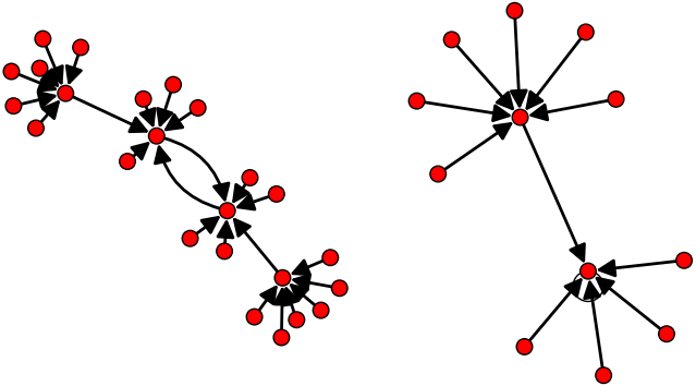 Figure 1
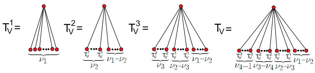 Figure 2