Scalable GAM using sparse variational Gaussian processes
Vincent Adam, Nicolas Durrande, ST John

TL;DR
This paper introduces a scalable Bayesian approach to generalized additive models using sparse variational Gaussian processes, enabling efficient and interpretable modeling of complex data.
Contribution
It presents a novel scalable Bayesian GAM framework with sparse GPs and variational inference, improving computational efficiency and model calibration.
Findings
Efficient inference for large datasets using sparse GPs.
Enhanced interpretability of GAM components.
Well-calibrated Bayesian uncertainty estimates.
Abstract
Generalized additive models (GAMs) are a widely used class of models of interest to statisticians as they provide a flexible way to design interpretable models of data beyond linear models. We here propose a scalable and well-calibrated Bayesian treatment of GAMs using Gaussian processes (GPs) and leveraging recent advances in variational inference. We use sparse GPs to represent each component and exploit the additive structure of the model to efficiently represent a Gaussian a posteriori coupling between the components.
Click any figure to enlarge with its caption.
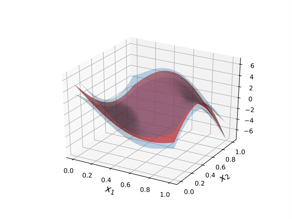 Figure 1
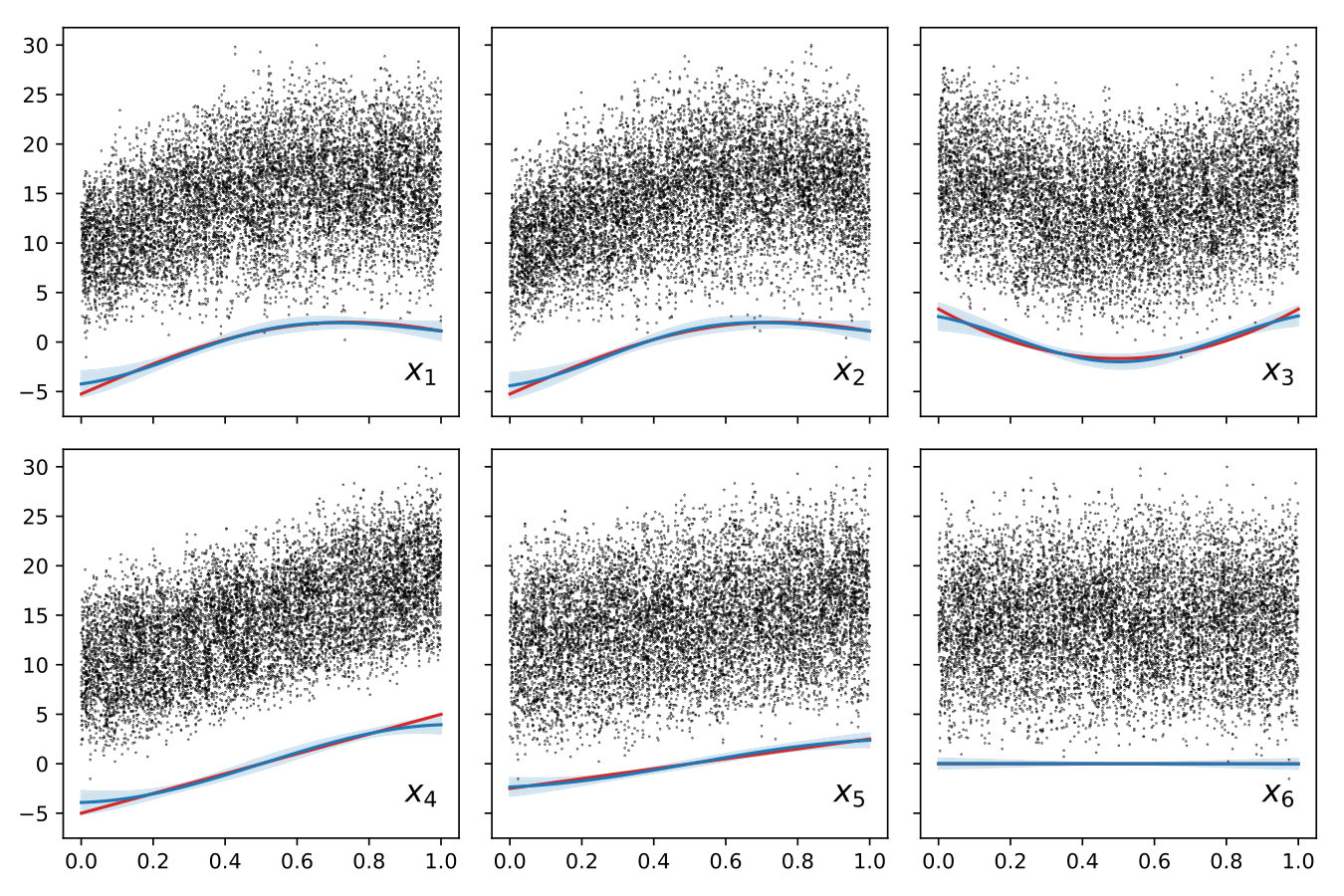 Figure 2
Peer Reviews
No public reviews on file for this paper yet. If you reviewed it on a platform where reviews are public (OpenReview, ICLR, NeurIPS, ICML), you can paste yours below so the community can read it here.
Videos
No videos yet. Explain this paper in a talk, walkthrough, or lecture? Add one.
Taxonomy
TopicsGaussian Processes and Bayesian Inference · Control Systems and Identification · Advanced Multi-Objective Optimization Algorithms
\theorembodyfont\theoremheaderfont\theorempostheader
: \theoremsep
\jmlrproceedingsAABI 20181st Symposium on Advances in Approximate Bayesian Inference, 2018
Scalable GAM using sparse variational Gaussian processes
\NameVincent Adam \[email protected]
\NameNicolas Durrande \[email protected]
\NameST John \[email protected]
\addrPROWLER.io
72 Hills Road
Cambridge
CB2 1LA
United Kingdom
Abstract
Generalized additive models (GAMs) are a widely used class of models of interest to statisticians as they provide a flexible way to design interpretable models of data beyond linear models. We here propose a scalable and well-calibrated Bayesian treatment of GAMs using Gaussian processes (GPs) and leveraging recent advances in variational inference. We use sparse GPs to represent each component and exploit the additive structure of the model to efficiently represent a Gaussian a posteriori coupling between the components.
keywords:
GAM, Gaussian Process, Variational Inference
1 Introduction
Generalized additive models (GAMs) are a class of interpretable regression models with non-linear yet additive predictors (Hastie, 2017). Their Bayesian treatment requires the specification of priors over functions. Here, we use Gaussian processes (GPs) (Rasmussen and Williams, 2006) and propose an approximate inference algorithm that is scalable with both the number of data points and additive components and that provides accurate posterior uncertainty estimates. We extend the variational pseudo-point GP approximation (Titsias, 2009; Bauer et al., 2016) to posterior dependencies across GPs. This approximation provides state-of-the art performance for GP regression and provides approximations to the posterior distributions in the form of a GP. This approach has been successfully extended to the multiple GP setting using a factorized (mean-field) approximation of the posterior across GPs (Saul et al., 2016; Adam et al., 2016). However, it suffers from the known variance underestimation of mean-field approximations and therefore can lead to poor predictions or can bias learning (Turner and Sahani, 2011). Adam (2017) introduced additional structure to the posterior distribution by allowing some coupling across the inducing variables of the different GPs but this was at the cost of scalability.
2 Background
2.1 Regression with multiple GPs
We consider models with additive predictor and factorizing likelihood , where are functions from . The specific form of the likelihood is arbitrary. We denote such that constitutes the joint distribution over the a priori independent processes. is the vector of function evaluations at . To simplify notation, when no argument is given, . We denote by the block-diagonal prior covariance matrix over . We are interested in computing the joint posterior .
2.2 Variational Inference
The classical variational lower bound (or ELBO) to the marginal likelihood is given by
[TABLE]
This is the optimization objective in the Variational Free Energy (VFE) approximation. We choose to be a multivariate normal distribution with mean and covariance , which is not an approximation in the conjugate likelihood setting. This leads to
[TABLE]
The expectation term in equation (2) is intractable in most cases and needs to be approximated. See Hensman et al. (2015) for deterministic approximations and Salimbeni and Deisenroth (2017) for stochastic approximations.
3 Optimal Gaussian posterior in variational inference
Following Opper and Archambeau (2009), we derive the expression for the optimal by noting that at the optimum, . This implies that
[TABLE]
3.1 Optimality in the additive case
In the additive case considered here, the gradient term in (3) is low-rank and can be parameterized by a vector as follows, with and :
[TABLE]
This parameterization requires values, equal to that of the classical single GP regression setting described in Opper and Archambeau (2009). It also inherits the non-convexity of this objective as highlighted by Khan et al. (2012).
3.2 Optimality in the sparse additive case
Following Adam et al. (2016) we introduce for each GP indexed by a set of ‘inducing points’ . The vector of associated function evaluations is given by . We also define the stacked vector .
Following Adam (2017), we parameterize . This choice leads to a simplification of the lower bound (2) as
[TABLE]
Saul et al. (2016) considered the mean field case with each factor parameterized as a multivariate normal distribution . This approach does not capture posterior dependencies across GPs. Adam (2017) parameterized as a multivariate normal distribution to include cross-GP coupling through the inducing variables . We extend this last approach but ask what the optimal should be. It turns out to be (see Appendix A):
[TABLE]
This form has again parameters which becomes an over-parameterization as soon as . Since we are interested in scalability, it is not of practical interest.
4 A new parameterization for
The second term of the sum in (6) can be expressed as with of size . Keeping this structure arising from the additivity of the model, we propose the parameterization
[TABLE]
with of size smaller than . This parameterization preserves the structure of the optimal covariance. It requires storing values, which is less than a direct representation of a Cholesky factor of that would require parameters.
5 Summary of complexities
Time and space complexity of the sparse variational algorithms are summarized in Table LABEL:table:complexity.
6 Related work
Variational inference for the multi-GP setting has so far only used the mean-field (MF) approximation as described in Saul et al. (2016). When posterior dependencies are a quantity of interest, a natural approach is to increase the complexity of the variational posterior to capture these dependencies. This often results in a prohibitive increase in the complexity of the inference. Different solutions have been proposed to tackle this problem. A first approach in Giordano et al. (2015) consists of a two-step scheme where MF inference is assumed to provide accurate posterior mean estimates. A perturbation analysis is then performed around the MF posterior means to provide second order (covariance) estimates. A second approach consists in ‘relaxing’ the MF approximation by extending the variational posterior with additional multiplicative terms capturing dependencies while keeping the computational complexity of the resulting inference scheme low (Tran et al., 2015; Hoffman and Blei, 2015). Our approach fits in this second family of extensions of the MF parameterization. It is tailored to the VFE approximation to GP models and leverages its sparsity to provide a fast and scalable inference algorithm.
7 Illustration
We consider a simple regression task consisting of approximating the following function: with (note that the last variable has no effect), given 5000 observation points uniformly distributed in the input space and a Gaussian observation noise with unit variance.
We choose a kernel dedicated to sensitivity analysis and tailored to the structure of the function at stake [Durrande et al. (2013)]. Given univariate squared exponential kernels we define the kernel as with
[TABLE]
Since the number of observations is relatively large and the kernel has an additive structure (it is the sum of 8 kernels), we choose the sparse additive model described above. We choose 16 regularly spaced one-dimensional inducing points for each kernel and 16 points distributed as a grid for the bi-dimensional kernel . The final model is obtained by maximizing the ELBO with respect to the variational parameters and the hyper-parameters of the . Given the structure of the model and the fact that inducing inputs are dedicated to model components, it is then possible to decompose the model predictions and to represent separately all the components of the ANOVA representation of the test function. Figure 1 shows that the model accurately approximates the test function and that the proposed framework is helpful to reveal its inner structure.
8 Conclusion
We presented a method that provides a fast, scalable and well-calibrated Bayesian treatment of GAMs. Although motivated by GAMs, our structured variational distribution may be used in models where the predictor is non-additive but where the posterior is well-approximated by a unimodal distribution.
Appendix A Optimal covariance in the additive case
We first define . From Opper and Archambeau (2009), we know that the optimal variational precision is structured as
[TABLE]
For factorizing likelihood and additive predictors, and defining , we have
[TABLE]
where has variance .
The gradient term in the optimal precision thus can be written as
[TABLE]
where is the indicator matrix of size with at location . With , this can be rewritten in matrix form:
[TABLE]
Appendix B ELBO evaluation: additive case
We parameterize the approximate posterior as
[TABLE]
with
[TABLE]
and optimize
[TABLE]
where
[TABLE]
B.1 Computing marginals of
[TABLE]
where
[TABLE]
To evaluate the ELBO we need, for each data point , the marginal . This corresponds to the diagonal elements of
[TABLE]
B.2 Computing the KL
[TABLE]
[TABLE]
In the end,
[TABLE]
B.3 Summary
Appendix C ELBO evaluation: sparse additive case
We parameterize an approximate posterior over the inducing values as
[TABLE]
with
[TABLE]
where . We optimize
[TABLE]
with
[TABLE]
C.1 Computing marginals of
We have
[TABLE]
where , so
[TABLE]
and
[TABLE]
Therefore
[TABLE]
The Cholesky decomposition of is of cost . Solving operations for each additive term costs a total of . Computing the marginal predictor variances then costs an extra . In total, the computational cost of posterior predictions is .
C.2 Computing the KL
As in the additive case, we have
[TABLE]
and
[TABLE]
In the end,
[TABLE]
C.3 Summary
The reference list from the paper itself. Each links out to its DOI / PubMed record.
- 1Adam (2017) Vincent Adam. Structured variational inference for coupled Gaussian processes. ar Xiv preprint ar Xiv:1711.01131 , 2017.
- 2Adam et al. (2016) Vincent Adam, James Hensman, and Maneesh Sahani. Scalable transformed additive signal decomposition by non-conjugate Gaussian process inference. In Machine Learning for Signal Processing (MLSP), 2016 IEEE 26th International Workshop on , pages 1–6. IEEE, 2016.
- 3Bauer et al. (2016) Matthias Bauer, Mark van der Wilk, and Carl Edward Rasmussen. Understanding probabilistic sparse Gaussian process approximations. In Advances in Neural Information Processing Systems , pages 1533–1541, 2016.
- 4Durrande et al. (2013) Nicolas Durrande, David Ginsbourger, Olivier Roustant, and Laurent Carraro. ANOVA kernels and RKHS of zero mean functions for model-based sensitivity analysis. Journal of Multivariate Analysis , 115:57–67, 2013.
- 5Giordano et al. (2015) Ryan J Giordano, Tamara Broderick, and Michael I Jordan. Linear response methods for accurate covariance estimates from mean field variational Bayes. In Advances in Neural Information Processing Systems , pages 1441–1449, 2015.
- 6Hastie (2017) Trevor J Hastie. Generalized additive models. In Statistical models in S , pages 249–307. Routledge, 2017.
- 7Hensman et al. (2015) James Hensman, Alexander Matthews, and Zoubin Ghahramani. Scalable variational gaussian process classification. JMLR , 2015.
- 8Hoffman and Blei (2015) Matthew Hoffman and David Blei. Stochastic structured variational inference. In Artificial Intelligence and Statistics , pages 361–369, 2015.