A continuous-time analysis of distributed stochastic gradient
Nicholas M. Boffi, Jean-Jacques E. Slotine

TL;DR
This paper studies how synchronization in distributed stochastic gradient algorithms reduces noise and improves convergence, using a biological analogy and providing theoretical and empirical evidence on non-convex objectives and neural networks.
Contribution
It introduces a quorum sensing-inspired analysis of synchronization effects, derives convergence bounds, and explores new algorithms with regularizing properties for distributed and non-distributed optimization.
Findings
Synchronization reduces noise in distributed SGD.
Coupling stabilizes higher noise levels and enhances convergence.
EASGD exhibits a surprising regularizing effect even in non-distributed settings.
Abstract
We analyze the effect of synchronization on distributed stochastic gradient algorithms. By exploiting an analogy with dynamical models of biological quorum sensing - where synchronization between agents is induced through communication with a common signal - we quantify how synchronization can significantly reduce the magnitude of the noise felt by the individual distributed agents and by their spatial mean. This noise reduction is in turn associated with a reduction in the smoothing of the loss function imposed by the stochastic gradient approximation. Through simulations on model non-convex objectives, we demonstrate that coupling can stabilize higher noise levels and improve convergence. We provide a convergence analysis for strongly convex functions by deriving a bound on the expected deviation of the spatial mean of the agents from the global minimizer for an algorithm based on…
Click any figure to enlarge with its caption.
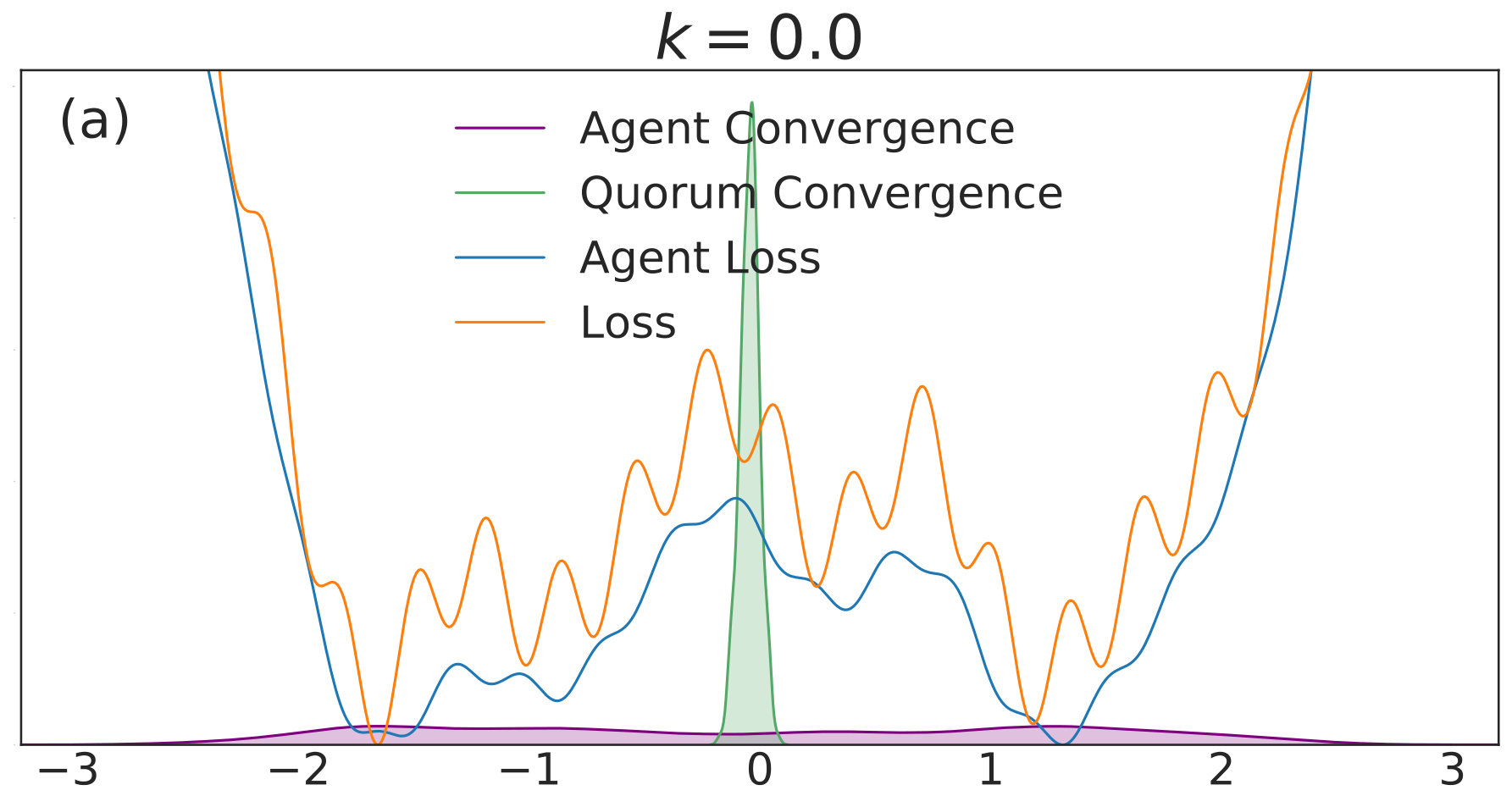 Figure 1
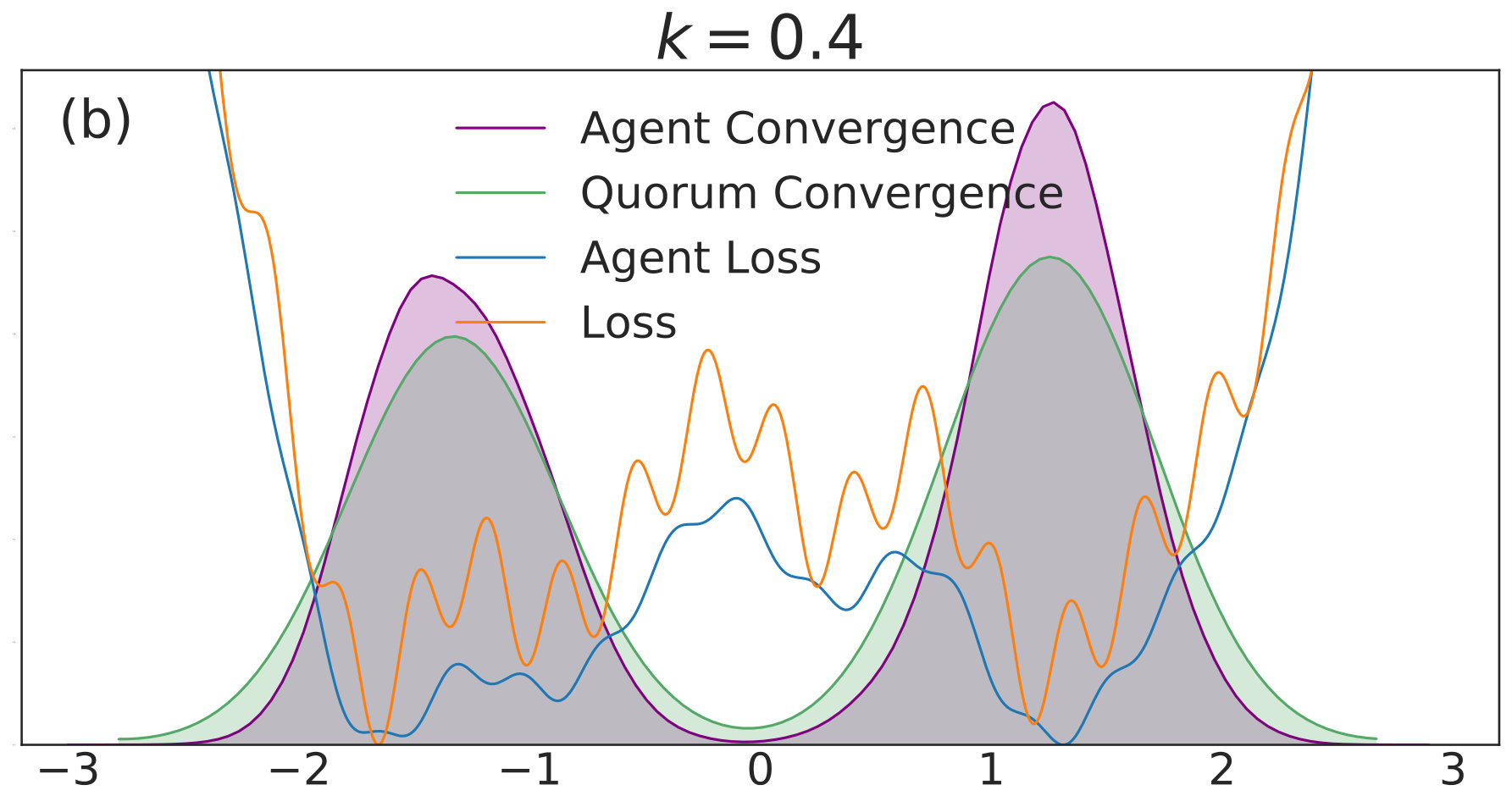 Figure 2
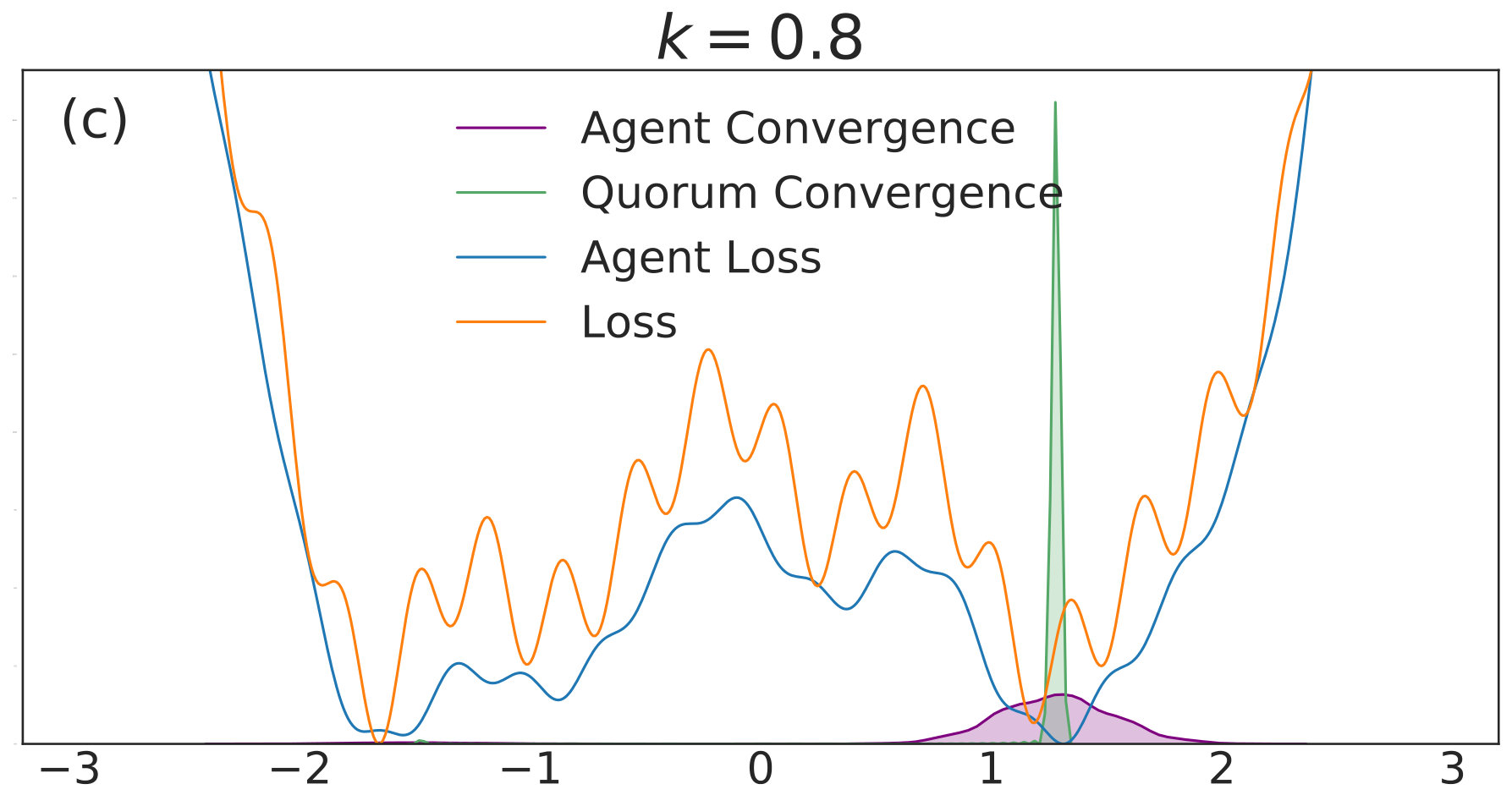 Figure 3
 Figure 4
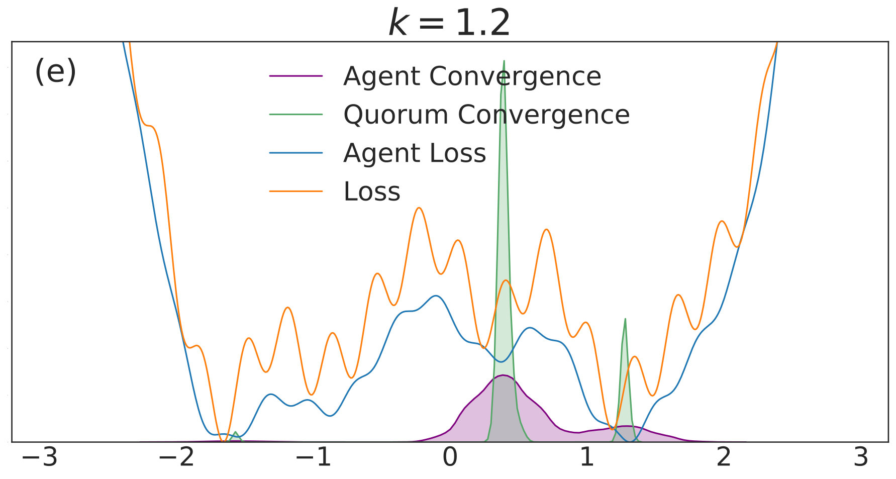 Figure 5
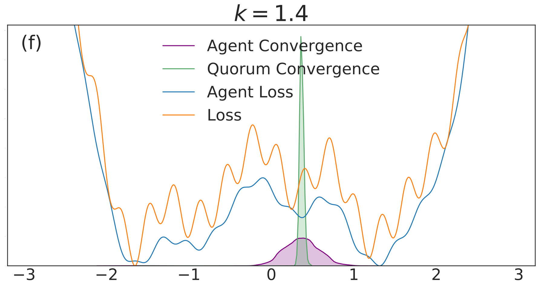 Figure 6
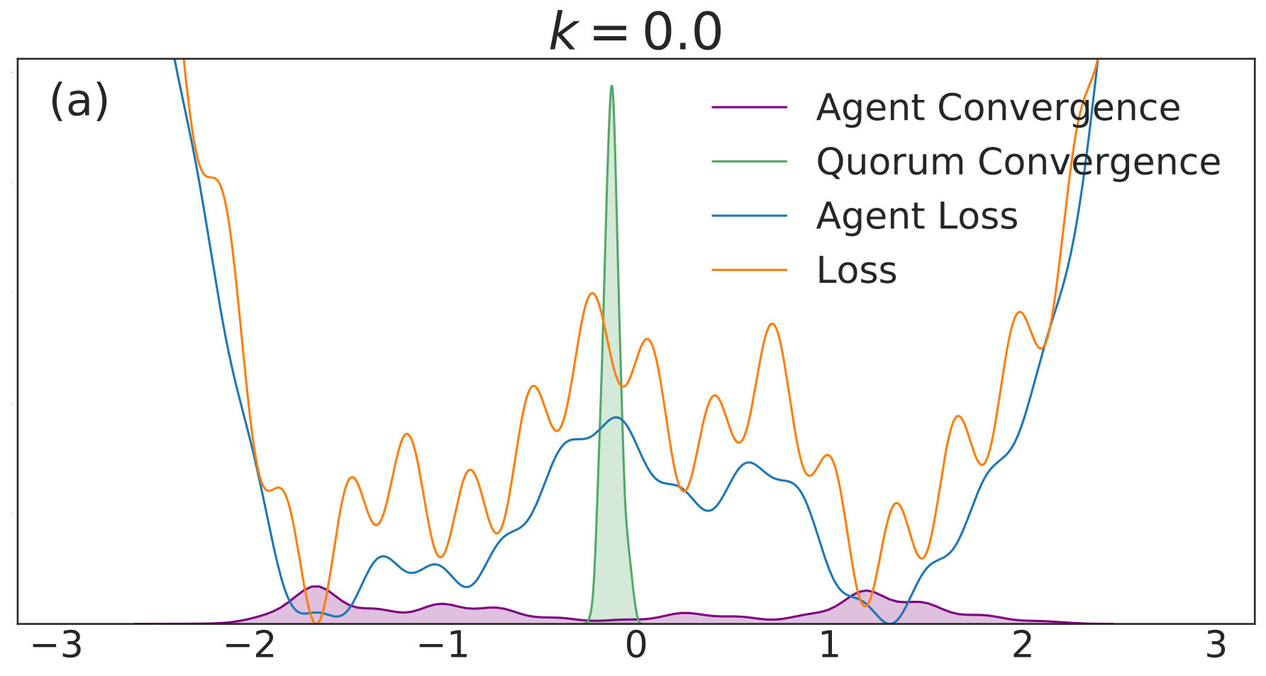 Figure 7
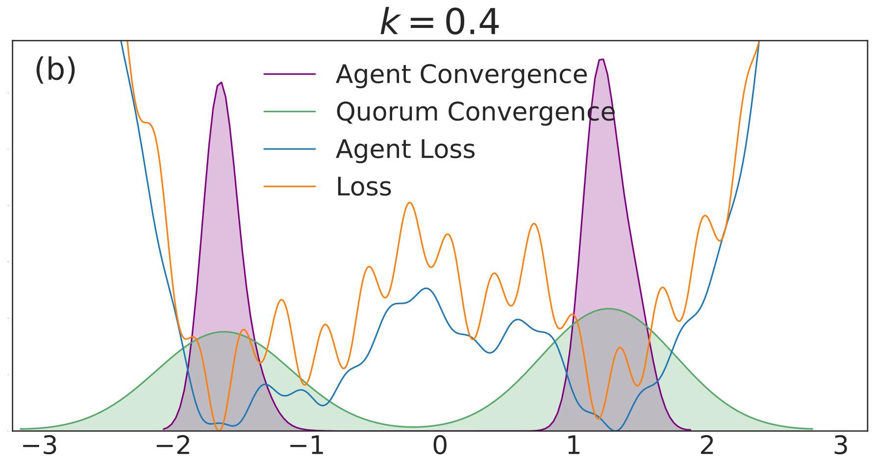 Figure 8
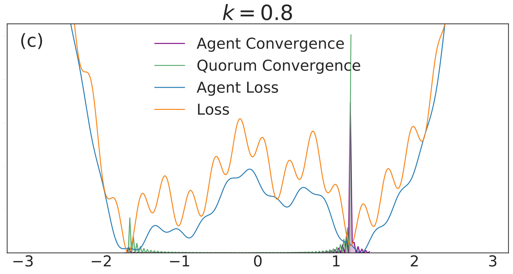 Figure 9
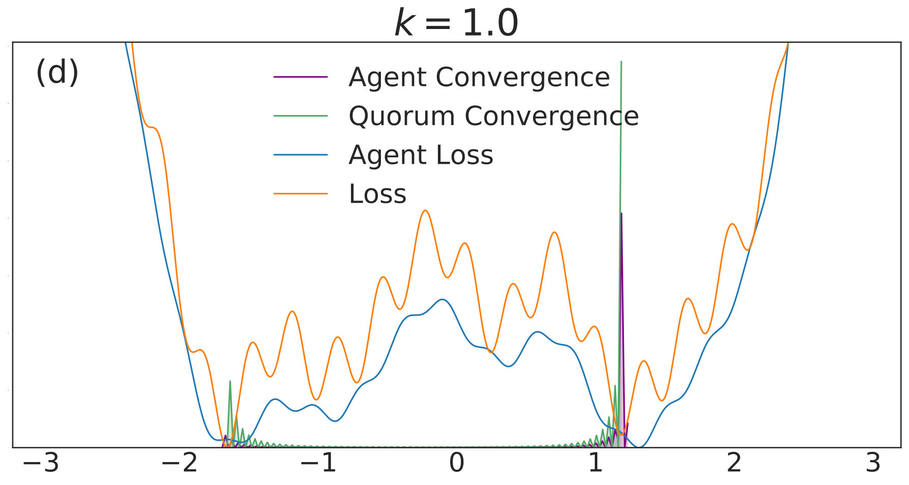 Figure 10
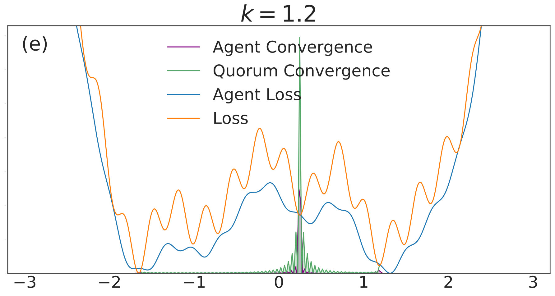 Figure 11
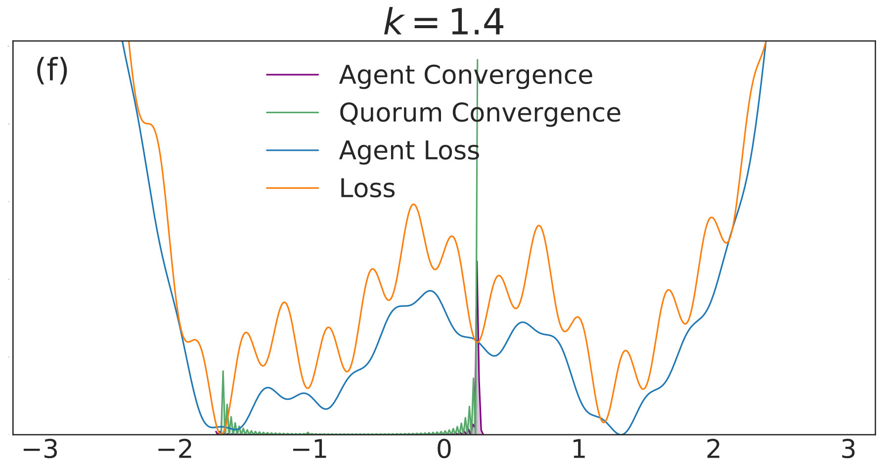 Figure 12
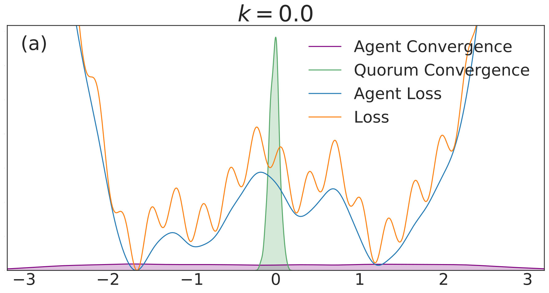 Figure 13
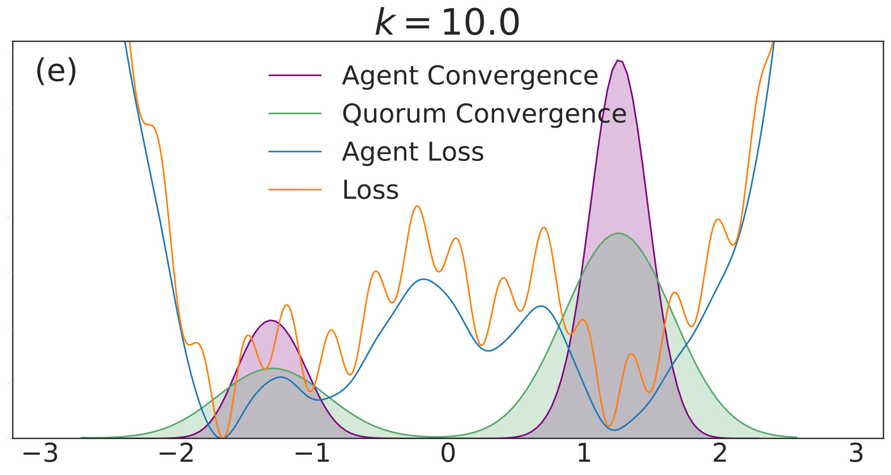 Figure 14
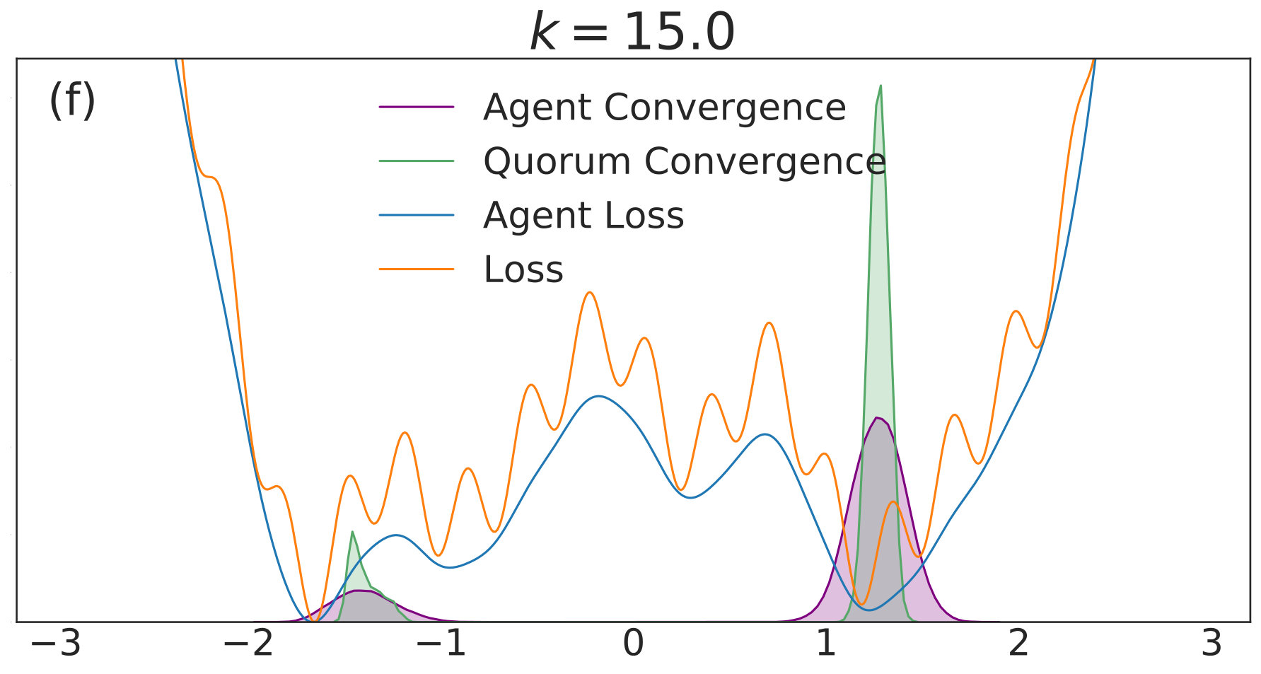 Figure 15
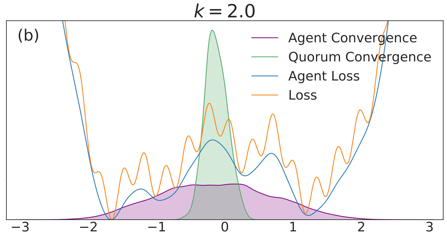 Figure 16
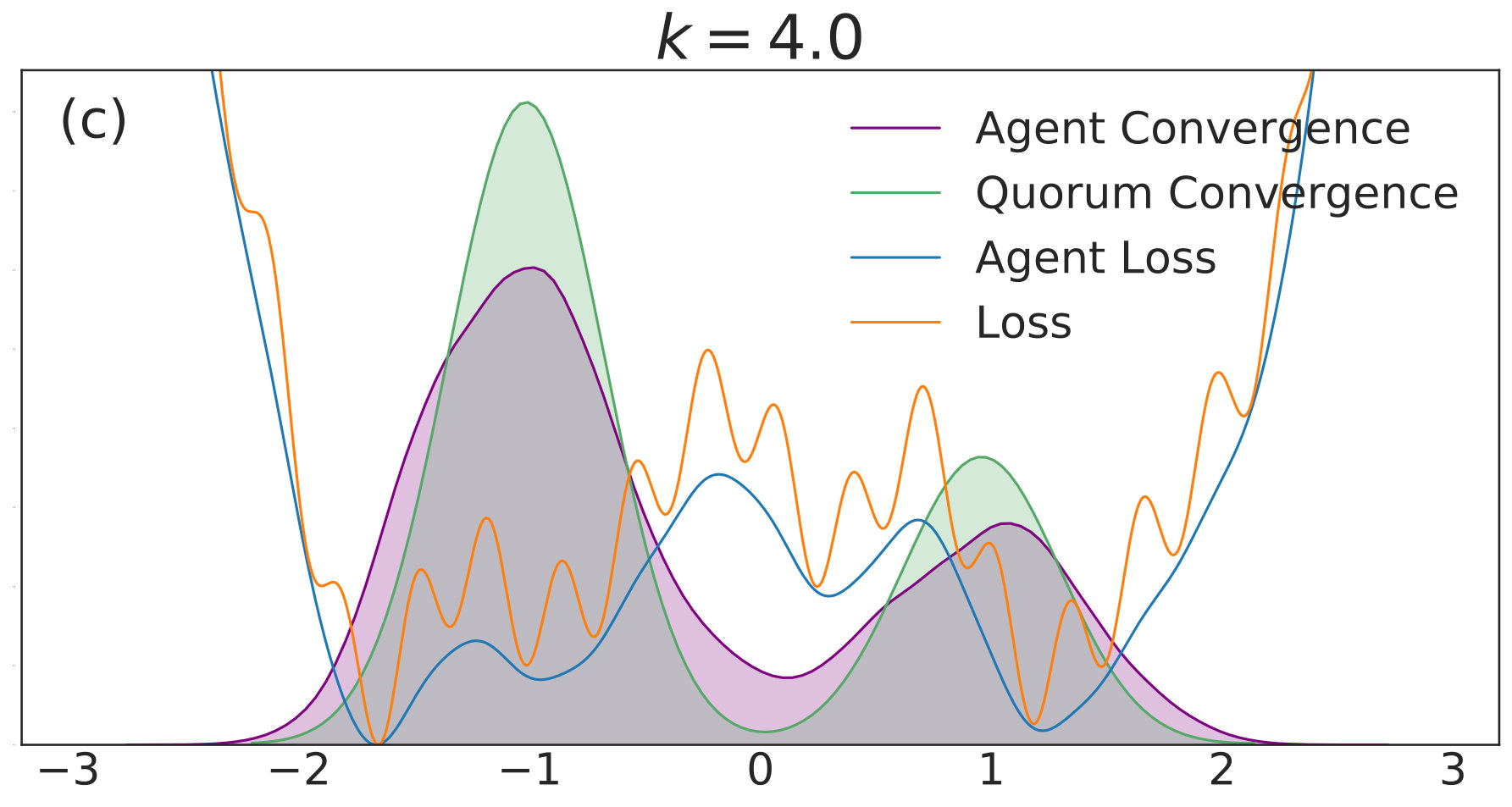 Figure 17
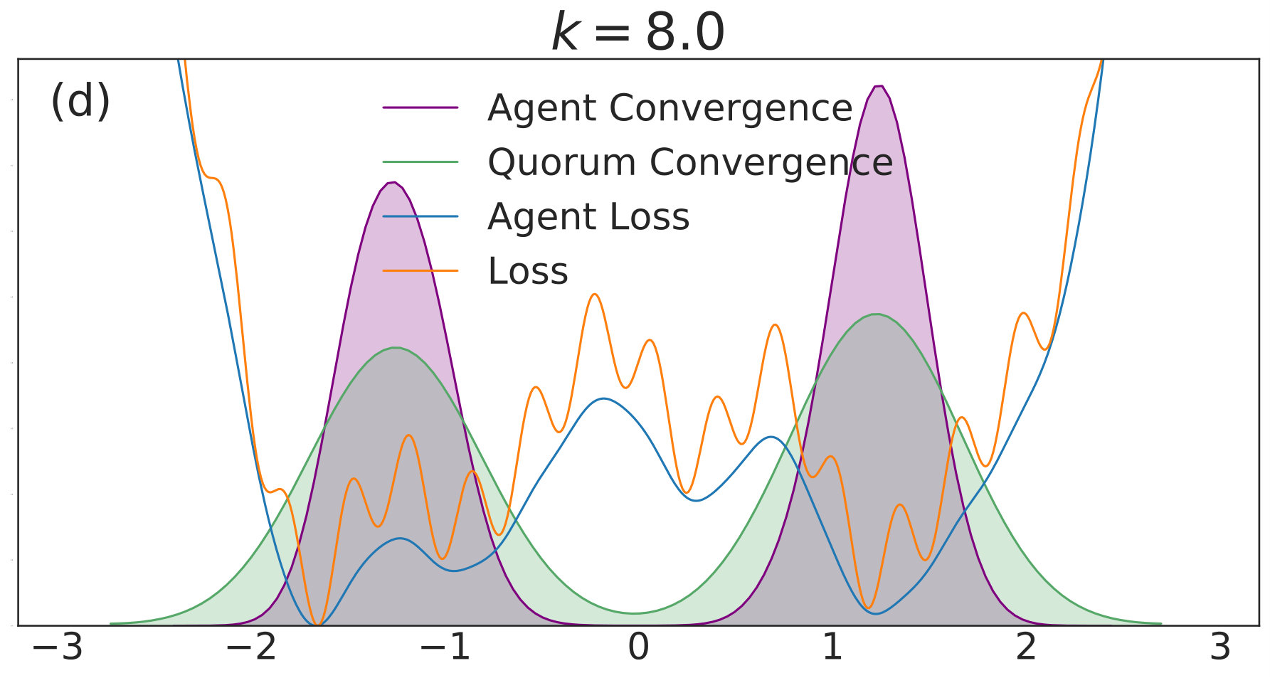 Figure 18
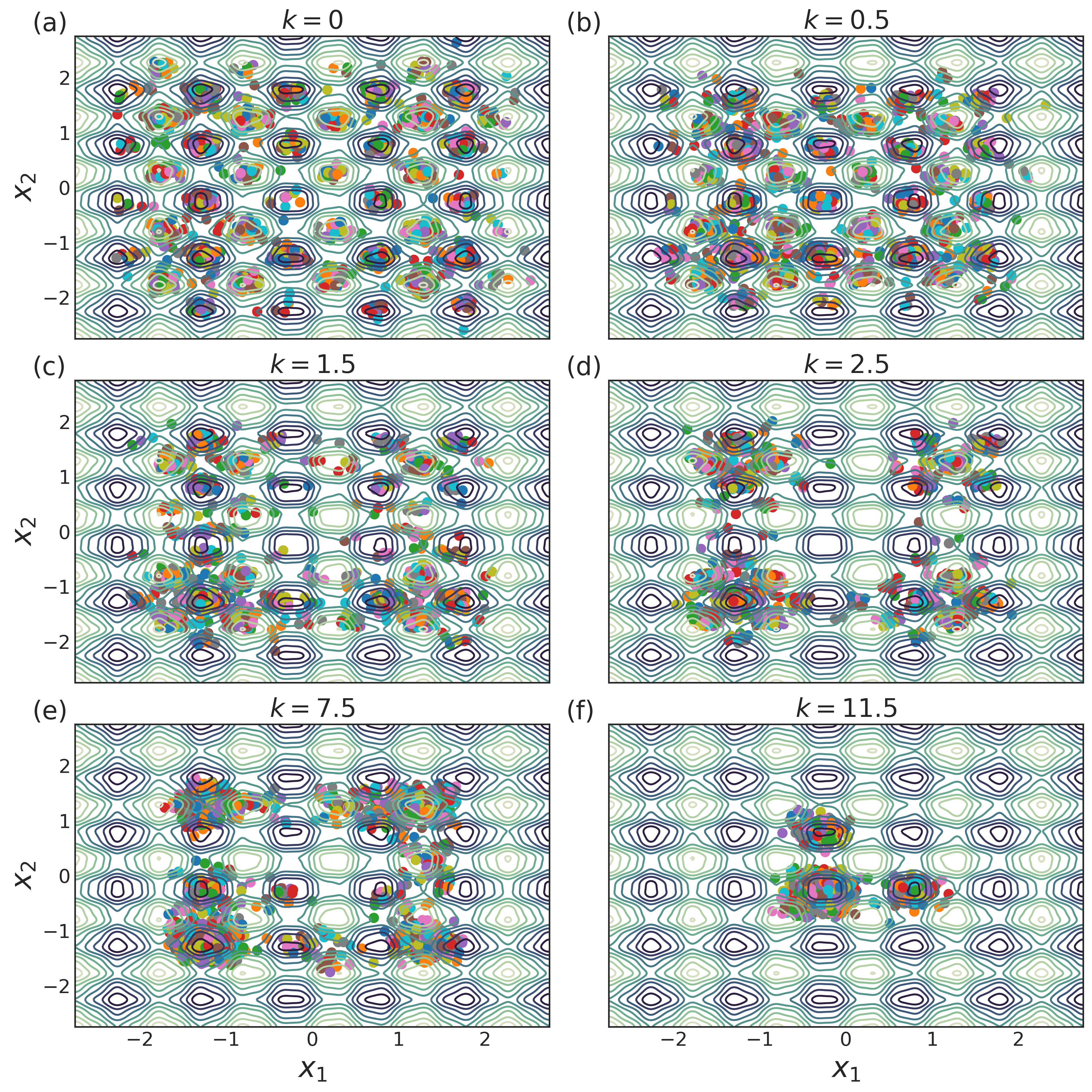 Figure 19
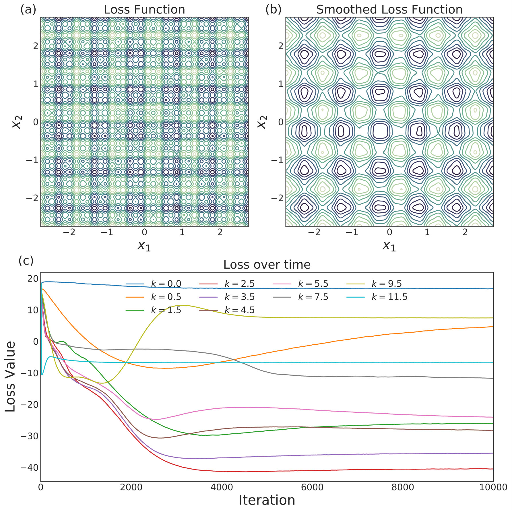 Figure 20
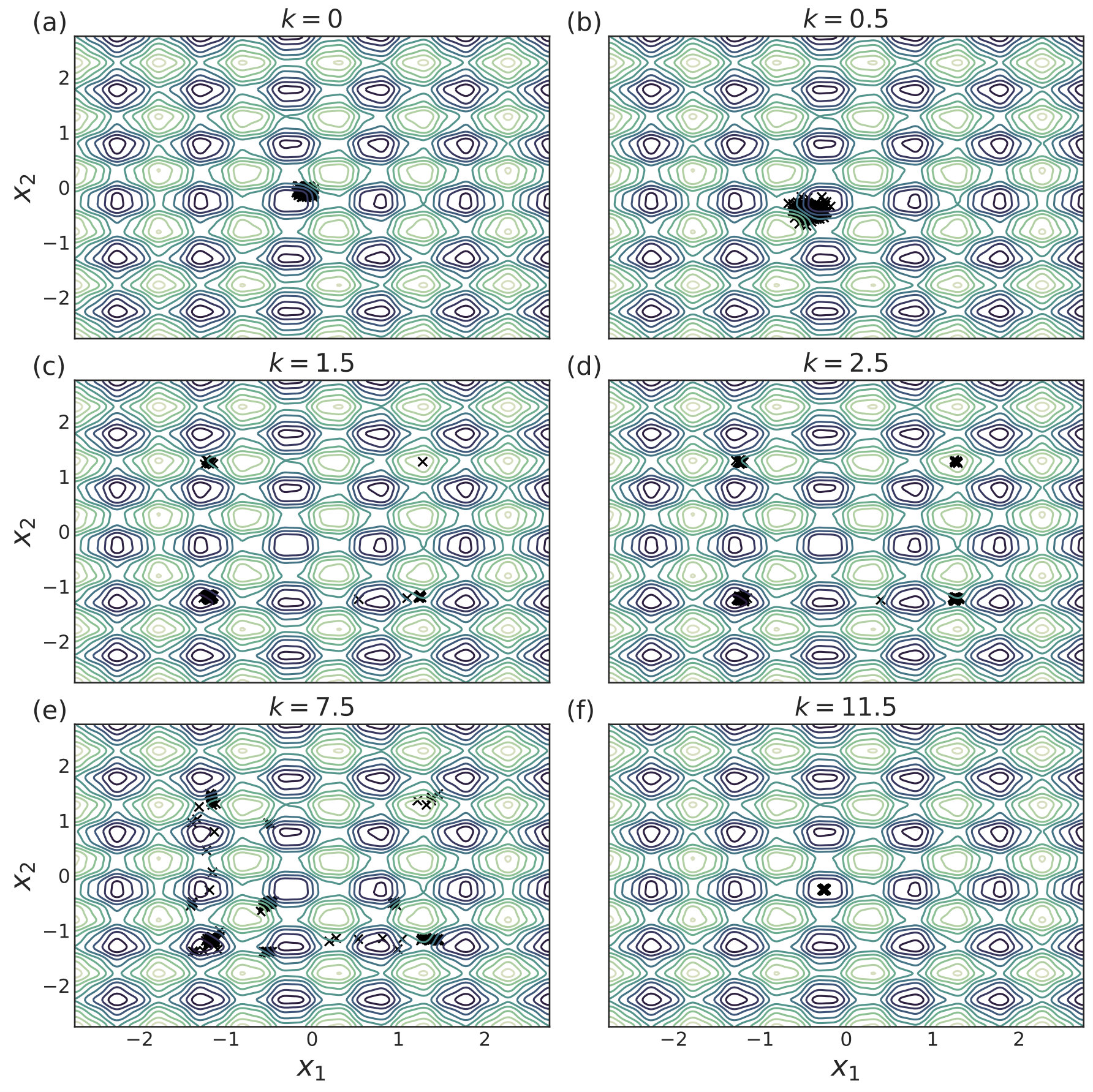 Figure 21
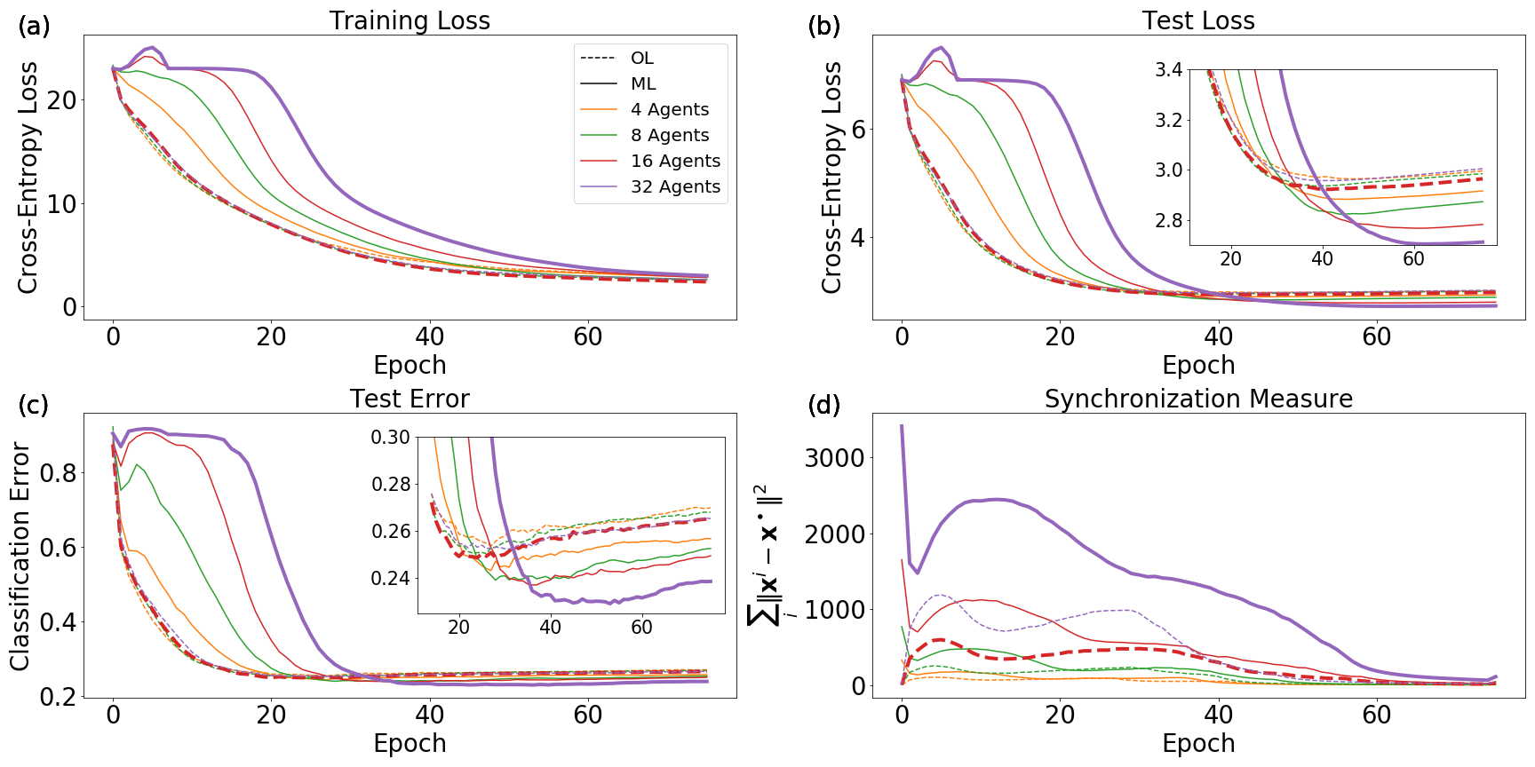 Figure 22
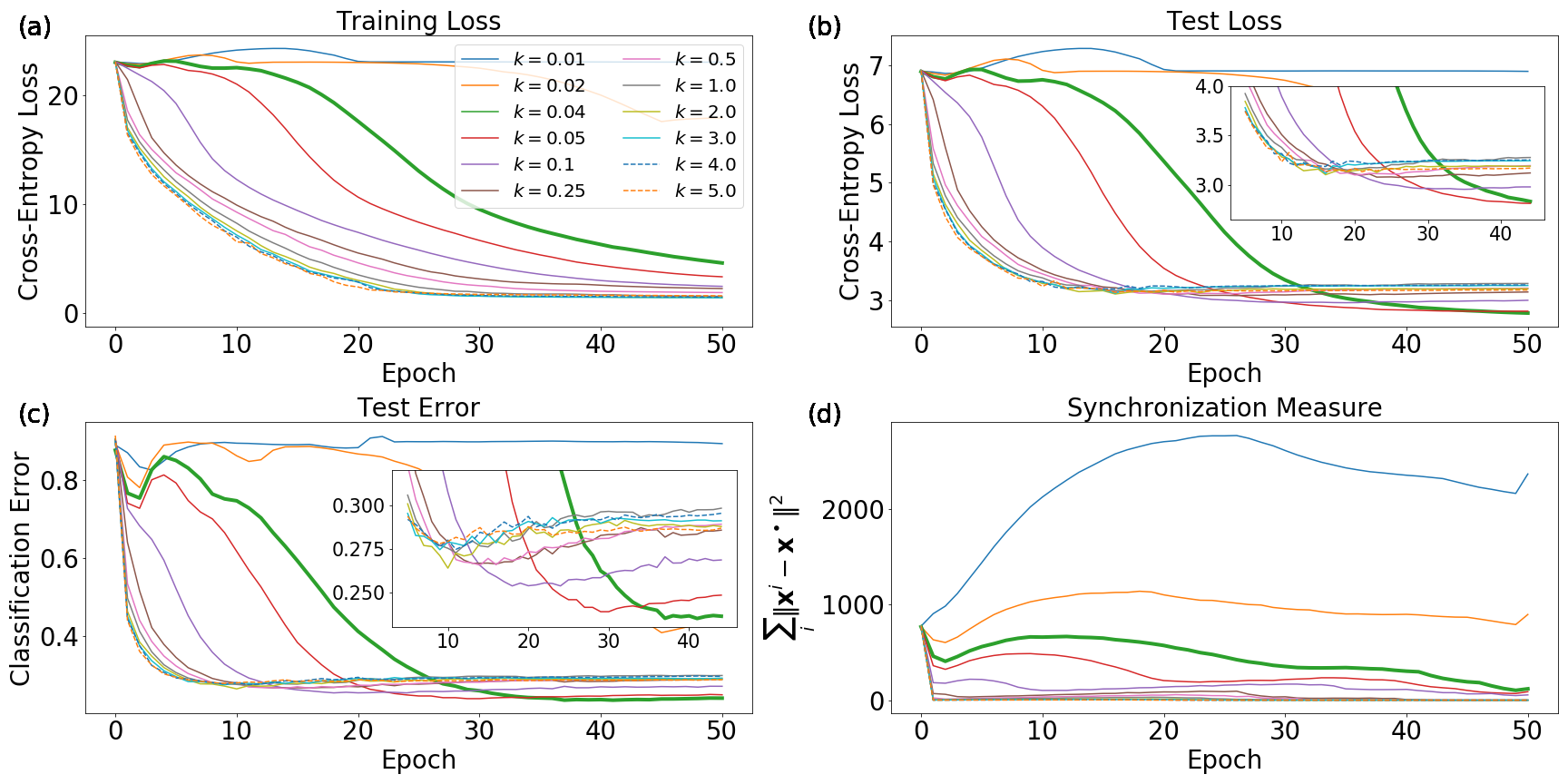 Figure 23
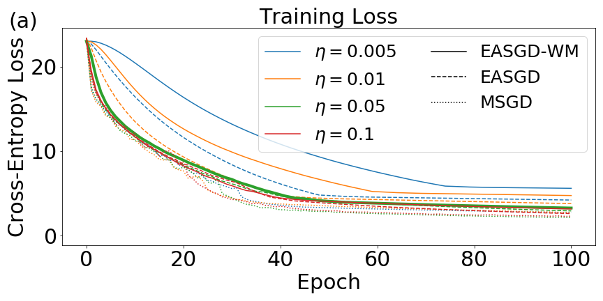 Figure 24
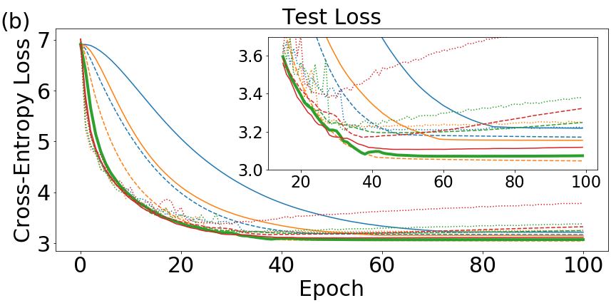 Figure 25
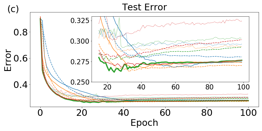 Figure 26
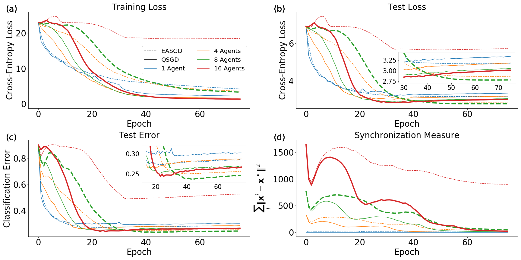 Figure 27
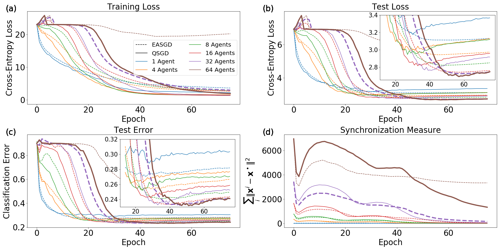 Figure 28
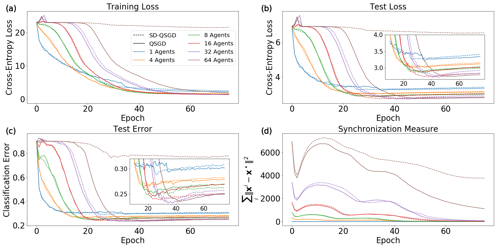 Figure 29
| Minimum Test Loss | Minimum Error | ||||||||||||
| EASGD-WM | 4.25 | 4.26 | 4.28 | 4.29 | 3.22 | 3.24 | .267 | .266 | .264 | .269 | .268 | .270 | |
| EASGD | 4.72 | 4.83 | 4.56 | 4.28 | 3.17 | 3.11 | .304 | .313 | .301 | .282 | .280 | .277 | |
| MSGD | 4.75 | 4.87 | 4.64 | 4.33 | 3.21 | 3.29 | .310 | .323 | .306 | .286 | .292 | .295 | |
| EASGD-WM | 4.09 | 5.15 | 4.03 | 4.12 | 3.15 | 3.10 | .262 | .259 | .253 | .261 | .267 | .257 | |
| EASGD | 4.57 | 5.75 | 4.27 | 4.14 | 3.04 | 3.22 | .297 | .300 | .280 | .275 | .263 | .283 | |
| MSGD | 4.59 | 5.81 | 4.48 | 4.46 | 3.22 | 3.33 | .300 | .307 | .294 | .294 | .287 | .301 | |
| EASGD-WM | 3.95 | 3.96 | 3.86 | 3.97 | 3.07 | 3.00 | .252 | .258 | .250 | .255 | .262 | .253 | |
| EASGD | 4.41 | 4.27 | 4.05 | 4.06 | 3.19 | 4.04 | .286 | .283 | .265 | .267 | .276 | .417 | |
| MSGD | 4.46 | 4.57 | 4.48 | 4.43 | 3.21 | 6.91 | .294 | .307 | .295 | .290 | .292 | 0.9 | |
| EASGD-WM | 4.08 | 4.01 | 4.04 | 4.05 | 3.11 | 3.15 | .267 | .264 | .268 | .265 | .268 | .269 | |
| EASGD | 4.24 | 4.23 | 4.14 | 4.13 | 3.17 | 6.91 | .282 | .283 | .277 | .272 | .280 | 0.9 | |
| MSGD | 4.62 | 4.55 | 4.22 | 4.47 | 3.38 | 6.91 | .288 | .307 | .287 | .288 | .301 | 0.9 | |
Peer Reviews
No public reviews on file for this paper yet. If you reviewed it on a platform where reviews are public (OpenReview, ICLR, NeurIPS, ICML), you can paste yours below so the community can read it here.
Videos
No videos yet. Explain this paper in a talk, walkthrough, or lecture? Add one.
Taxonomy
MethodsStochastic Gradient Descent
A continuous-time analysis of distributed stochastic gradient
Nicholas M. Boffi
John A. Paulson School of Engineering and Applied Sciences
Harvard University
Cambridge, MA 02138
&Jean-Jacques E. Slotine
Nonlinear Systems Laboratory
Massachusetts Institute of Technology
Cambridge, MA 02139
Abstract
We analyze the effect of synchronization on distributed stochastic gradient algorithms. By exploiting an analogy with dynamical models of biological quorum sensing – where synchronization between agents is induced through communication with a common signal – we quantify how synchronization can significantly reduce the magnitude of the noise felt by the individual distributed agents and by their spatial mean. This noise reduction is in turn associated with a reduction in the smoothing of the loss function imposed by the stochastic gradient approximation. Through simulations on model non-convex objectives, we demonstrate that coupling can stabilize higher noise levels and improve convergence. We provide a convergence analysis for strongly convex functions by deriving a bound on the expected deviation of the spatial mean of the agents from the global minimizer for an algorithm based on quorum sensing, the same algorithm with momentum, and the Elastic Averaging SGD (EASGD) algorithm. We discuss extensions to new algorithms that allow each agent to broadcast its current measure of success and shape the collective computation accordingly. We supplement our theoretical analysis with numerical experiments on convolutional neural networks trained on the CIFAR-10 dataset, where we note a surprising regularizing property of EASGD even when applied to the non-distributed case. This observation suggests alternative second-order in-time algorithms for non-distributed optimization that are competitive with momentum methods.
1 Introduction
Stochastic gradient descent (SGD) and its variants have become the de-facto algorithms for large-scale machine learning applications such as deep neural networks [Bottou, 2010, Goodfellow et al., 2016, LeCun et al., 2015, Mallat, 2016]. SGD is used to optimize finite-sum loss functions, where a stochastic approximation to the gradient is computed using only a random selection of the input data points. Well-known results on almost-sure convergence rates to global minimizers for strictly convex functions and to stationary points for non-convex functions exist under sufficient regularity conditions [Bottou, 1998, Robbins and Siegmund, 1971]. Classic work on iterate averaging for SGD [Polyak and Juditsky, 1992] and other more recent extensions [Defazio et al., 2014, Roux et al., 2012, Bach and Moulines, 2013, Schmidt et al., 2017] can improve convergence under a set of reasonable assumptions typically satisfied in the machine learning setting. Convergence proofs rely on a suitably chosen decreasing step size; for constant step sizes and strictly convex functions, the parameters ultimately converge to a distribution peaked around the optimum.
For large-scale machine learning applications, parallelization of SGD is a critical problem of significant modern research interest [Dean et al., 2012, Recht and Ré, 2013, Recht et al., 2011, Chaudhari et al., 2017]. Recent work in this direction includes the Elastic Averaging SGD (EASGD) algorithm, in which distributed agents coupled through a common signal optimize the same loss function. EASGD can be derived from a single SGD step on a global variable consensus objective with a quadratic penalty, and the common signal takes the form of an average over space and time of the parameter vectors of the individual agents [Zhang et al., 2015, Boyd et al., 2010]. At its core, the EASGD algorithm is a system of identical, coupled, discrete-time dynamical systems. And indeed, the EASGD algorithm has exactly the same structure as earlier mathematical models of synchronization [Russo and Slotine, 2010, Chung and Slotine, 2009] inspired by quorum sensing in bacteria [Miller and Bassler, 2001, Waters and Bassler, 2005]. In these models, which have typically been analyzed in continuous-time, the dynamics of the common (quorum) signal can be arbitrary [Russo and Slotine, 2010], and in fact may simply consist of a weighted average of individual signals. Motivated by this immediate analogy, we present here a continuous-time analysis of distributed stochastic gradient algorithms, of which EASGD is a special case. A significant focus of this work is the interaction between the degree of synchronization of the individual agents, characterized rigorously by a bound on the expected distance between all agents and governed by the coupling strength, and the amount of noise induced by their stochastic gradient approximations.
The effect of coupling between identical continuous-time dynamical systems has a rich history. In particular, synchronization phenomena in such coupled systems have been the subject of much mathematical [Wang and Slotine, 2005], biological [Russo and Slotine, 2010], neuroscientific [Tabareau et al., 2010], and physical interest [Javaloyes et al., 2008]. In nonlinear dynamical systems, synchronization has been shown to play a crucial role in protection of the individual systems from independent sources of noise [Tabareau et al., 2010]. The interaction between synchronization and noise has also been posed as a possible source of regularization in biological learning, where quorum sensing-like mechanisms could be implemented between neurons through local field potentials [Bouvrie and Slotine, 2013]. Given the significance of stochastic gradient [Zhang et al., 2018b] and externally injected [Neelakantan et al., 2015] noise in regularization of large-scale machine learning models such as deep networks [Zhang et al., 2017], it is natural to expect that the interplay between synchronization of the individual agents and the noise from their stochastic gradient approximations is of central importance in distributed SGD algorithms.
Recently, there has been renewed interest in a continuous-time view of optimization algorithms [Wilson et al., 2016, Wibisono et al., 2016, Wibisono and Wilson, 2015, Betancourt et al., 2018]. Nesterov’s accelerated gradient method [Nesterov, 1983] was fruitfully analyzed in continuous-time in Su et al. [2014], and a unifying extension to other algorithms can be found in Wibisono et al. [2016]. Continuous-time analysis has also enabled discrete-time algorithm development through classical discretization techniques from numerical analysis [Zhang et al., 2018a]. This paper further adds to this line of work by deriving new results with the mathematical tools afforded by the continuous-time view, such as stochastic calculus and nonlinear contraction analysis [Lohmiller and Slotine, 1998].
The paper is organized as follows. In Sec. 2, we provide some necessary mathematical preliminaries: a review of SGD in continuous-time, a continuous-time limit of the EASGD algorithm, a review of stochastic nonlinear contraction theory, and a statement of some needed assumptions. In Sec. 3, we demonstrate that the effect of synchronization of the distributed SGD agents is to reduce the magnitude of the noise felt by each agent and by their spatial mean. We derive this for an algorithm where all-to-all coupling is implemented through communication with the spatial mean of the distributed parameters, and we refer to this algorithm as quorum SGD (QSGD). In the appendix, a similar derivation is presented with arbitrary dynamics for the quorum variable, of which EASGD is a special case. In Sec. 4, we connect this noise reduction property with a recent analysis in Kleinberg et al. [2018], which shows SGD can be interpreted as performing gradient descent on a smoothed loss in expectation. We use this derivation to garner intuition about the qualitative performance of distributed SGD algorithms as the coupling strength is varied, and we verify this intuition with simulations on model nonconvex loss functions in low and high dimensions. In Sec. 5, we provide new convergence results for QSGD, QSGD with momentum, and EASGD for a strongly convex objective. In Sec. 6, we explore the properties of EASGD and QSGD on deep neural networks, and in particular, test the stability and performance of variants proposed throughout the paper. We also propose a new class of second-order in time algorithms motivated by the EASGD algorithm with a single agent, which consists of standard SGD coupled in feedback to the output of a nonlinear filter of the parameters. We close with some concluding remarks in Sec. 7.
2 Mathematical preliminaries
In this section, we provide a brief review of the necessary mathematical tools employed in this work.
2.1 Convex optimization
For the convergence proofs in Sec. 5, and for synchronization of momentum methods, we will require a few standard definitions from convex optimization.
Definition 2.1**.**
(Strong Convexity) A function is -strongly convex with if its Hessian is uniformly lower bounded by with respect to the positive semidefinite order, for all .
Definition 2.2**.**
(L-Smoothness) A function is -smooth with if its Hessian is uniformly upper bounded by with respect to the positive semidefinite order, for all .
2.2 Stochastic gradient descent in discrete-time
Minibatch SGD has been essential for training large-scale machine learning models such as deep neural networks, where empirical risk minimization leads to finite-sum loss functions of the form
[TABLE]
Above, is the input data example and the vector holds the model parameters. In the typical machine learning setting where is very large, the gradient of requires gradient computations of , which is prohibitively expensive.
To avoid this calculation, a stochastic gradient is computed by taking a random selection of size , typically known as a minibatch. It is simple to see that the stochastic gradient
[TABLE]
is an unbiased estimator of the true gradient. The parameters are updated according to the iteration
[TABLE]
By adding and subtracting the true gradient, the SGD iteration can be rewritten
[TABLE]
where is a data-dependent noise term. can be taken to be Gaussian under a central limit theorem argument, assuming that the size of the minibatch is large enough [Jastrzȩbski et al., 2017, Mandt et al., 2015]. is then given by the variance of a single-element stochastic gradient
[TABLE]
2.3 Stochastic gradient descent in continuous-time
A significant difficulty in a continuous-time analysis of SGD is formulating an accurate stochastic differential equation (SDE) model. Recent works have proved rigorously [Hu et al., 2017, Feng et al., 2018, Li et al., 2018] that the sequence of values generated by the SDE
[TABLE]
approximates the SGD iteration with weak error , where is a Wiener process, denotes the Euclidean 2-norm111For the remainder of this paper, unless otherwise specified, we will use to denote the 2-norm., and where . Dropping the small term proportional to reduces the weak error to [Hu et al., 2017]. This leads to the SDE
[TABLE]
Equation (2) has appeared in a number of recent works [Mandt et al., 2017, 2016, 2015, Chaudhari and Soatto, 2018, Chaudhari et al., 2018, Jastrzȩbski et al., 2017], and is generally obtained by making the replacement and in (1), as a sort of reverse Euler-Maruyama discretization [Kloeden and Platen, 1992].
2.4 EASGD in continuous-time
Following [Zhang et al., 2015], we provide a brief introduction to the EASGD algorithm, and convert the resulting sequences to continuous-time. We imagine a distributed optimization setting with agents and a single master. We are interested in solving a stochastic optimization problem
[TABLE]
where is the vector of parameters and is a random variable representing the stochasticity in the objective. This is equivalent to the distributed optimization problem [Boyd et al., 2010]
[TABLE]
where each is a local vector of parameters and is the quorum variable. The quadratic penalty ensures that all local agents remain close to , and sets the coupling strength. Smaller values of allow for more exploration, while larger values ensure a greater degree of synchronization. Intuitively, the interaction between agents mediated by is expected to help individual trajectories escape local minima, saddle points, and flat regions, unless they all fall into the same deep or wide minimum together.
We assume the expectation in (2.4) is approximated by a sum over input data points, and that the stochastic gradient is computed by taking a minibatch of size . After taking an SGD step, the updates for each agent and the quorum variable become
[TABLE]
where and . Transferring to the continuous-time limit, these equations become,
[TABLE]
with . Note that in (5), the dynamics of represent a simple low-pass filter of the center of mass (spatial mean) variable . In the limit of large , the dynamics of this filter will be much faster than the SGD dynamics, and the continuous-time EASGD system can be approximately replaced by
[TABLE]
We refer to (6) as Quorum SGD (QSGD), and it will be a significant focus of this work.
2.5 Background on nonlinear contraction theory
The main mathematical tool used in this work is nonlinear contraction theory, a form of incremental stability for nonlinear systems. In particular, we specialize to the case of time- and state-independent metrics; further details can be found in Lohmiller and Slotine [1998].
Definition 2.3**.**
(Contraction) The nonlinear dynamical system
[TABLE]
with and is said to be contracting with rate and invertible metric transformation if the symmetric part of the generalized Jacobian
[TABLE]
is uniformly negative definite for all and all . Above, subscript denotes the symmetric part of a matrix, . Equivalently, the system is said to be contracting in the corresponding metric .
If condition (8) is satisfied, all trajectories exponentially converge to one another regardless of initial conditions. That is, for two solutions and of (7),
[TABLE]
where . Intuitively, because of the property (9), a nonlinear system is called contracting if differences in system trajectories due to initial conditions and temporary disturbances are exponentially forgotten. This behavior is proved differentially, by considering the time evolution of the squared Euclidean norm of the virtual displacement , which formally obeys the differential equation [Lohmiller and Slotine, 1998]. As an immediate and powerful corollary, if the system is contracting and a single trajectory is known, then all trajectories must converge to the single known trajectory exponentially.
In this work, we will interchangeably refer to , the system, and the generalized Jacobian as contracting depending on the context. In particular, for stochastic differential equations, we will refer to as contracting if the deterministic system is contracting. Two specific robustness results for contracting systems needed for the derivations in this work are summarized below.
Lemma 2.1**.**
Consider the dynamical system (7), and assume that it is contracting with metric transformation and contraction rate . Let denote the condition number of , where denotes the induced matrix 2-norm. Consider the perturbed dynamical system
[TABLE]
Then, for a solution of (7) and a solution of (10), with ,
[TABLE]
Furthermore, if with and , then after exponential transients of rates and ,
[TABLE]
Proof.
See point (vii) of “linear properties of generalized contraction analysis” in Lohmiller and Slotine [1998] for the derivation of (11). From (11), . Convolving with the right-hand side yields the inequality
[TABLE]
Noting that yields the result (12). ∎
Theorem 2.1**.**
Consider the stochastic differential equation
[TABLE]
with and where denotes an -dimensional Wiener process. Assume that there exists a positive definite metric such that with , and that is contracting in this metric. Further assume that where . Then, for two trajectories and driven by independent sources of noise with stochastic initial conditions given by a probability distribution ,
[TABLE]
where denotes the unit ramp (or ReLU) function. The expectation on the left-hand side is over the noise for all , and the expectation on the right-hand side is over the distribution of initial conditions.
See Pham et al. [2009], Thm. 2 for a proof of Thm. 2.1. A corollary that will be useful in Sec. 5 is as follows.
Corollary 2.1**.**
Assume that the conditions of Thm. 2.1 are satisfied. Then, for a trajectory of (7) and a trajectory of (14),
[TABLE]
Cor. 2.1 is obtained by following the proof of Thm. 2 in Pham et al. [2009] with the restriction that one system is deterministic. To reduce the appearance of decaying exponential terms, in applications of Thm. 2.1, Cor. 2.1, and other related contraction-based bounds, we will simply state the final constant and the corresponding rate of exponential transients. The conditions of Thm. 2.1 are worthy of their own definition.
Definition 2.4**.**
(Stochastic contraction) If the conditions of Thm. 2.1 are satisfied, the system (14) is said to be stochastically contracting in the metric (or with metric transformation ) with bound and rate .
In this work, we will also make use of an extension of contraction known as partial contraction originally introduced in Wang and Slotine [2005]. The procedure is summarized below.
Theorem 2.2**.**
Consider the nonlinear dynamical system (7) – not assumed to be contracting – and consider a contracting auxiliary system of the form
[TABLE]
with the requirement that .222For example, say with a symmetric and uniformly positive definite matrix. Then satisfies this restriction requirement. The system is also contracting in , as the symmetric part of the Jacobian uniformly. On the other hand, the system has Jacobian , which has symmetric part with unknown definiteness without further assumptions on . Assume a single trajectory of (15) is known. Then all trajectories of (7) converge to .
Proof.
By assumption, (15) is contracting, and so all trajectories converge to . Because , any solution of (7) is also a solution of (15), and hence must converge to . ∎
We will commonly refer to the auxiliary system in the above theorem as a virtual system, and is said to be partially contracting. Thm. 2.2 enables the application of contraction to systems which in themselves are not contracting, but can be embedded in a virtual system which is.
This notion also extends to stochastic systems through the use of stochastic contraction. If a stochastically contracting system
[TABLE]
can be found such that and , then trajectories of (16) can be compared to trajectories of (7) through the application of Cor. 2.1 or (14) through the application of Thm. 2.1.
2.6 Assumptions
We require two main assumptions about the objective function , both of which have been employed in previous work analyzing synchronization and noise in nonlinear systems [Tabareau et al., 2010]. The first is an assumption on the nonlinearity of the components of the gradient.
Assumption 2.1**.**
Assume that the Hessian matrix of each component of the negative gradient has bounded maximum eigenvalue, for all .
The second assumption is a condition on the robustness of the distributed gradient flows studied in this work to small, potentially stochastic perturbations.
Assumption 2.2**.**
Consider two dynamical systems
[TABLE]
where is a continuous-time stochastic process dependent on a parameter and is a real coefficient dependent on a parameter . Denote by the solution to (17) and by the solution to (18) with the same initial condition, . We assume that and implies that almost surely.
Continuous dependence of trajectories on parameters of the dynamics in the sense of Assumption 2.2 can be characterized for deterministic systems through continuity assumptions on the dynamics – see, for example, Section 3.2 in Khalil [2002] – here we assume a natural stochastic extension. Assumption 2.2 has been verified for FitzHugh-Nagumo oscillators where is a white noise process [Tuckwell and Rodriguez, 1998], and validated in simulation for more complex nonlinear oscillators [Tabareau et al., 2010]. We remark that implies that almost surely, and hence that almost surely.
3 Synchronization and noise
In this section, we analyze the interaction between synchronization of the distributed QSGD agents and the noise they experience. We begin with a derivation of a quantitative measure of synchronization that applies to a class of distributed SGD algorithms involving coupling to a common external signal with no communication delays. We then present the section’s primary contribution, which will serve as a basis for the theory in the remainder of the paper, as well as for the intuition for various experiments.
3.1 A measure of synchronization
We now present a simple theorem on synchronization in the deterministic setting, which will allow us to prove a bound on synchronization in the stochastic setting using Thm. 2.1.
Theorem 3.1**.**
Consider the coupled gradient descent system
[TABLE]
where represents a common external signal. Let denote the maximum eigenvalue of . For , the individual trajectories synchronize exponentially with rate regardless of initial conditions.
Proof.
Consider the auxiliary virtual system
[TABLE]
where is an external input. Note that with , we recover (19) – i.e., (20) admits the trajectories of each agent as particular solutions. The Jacobian of (20) is given by
[TABLE]
Equation (21) is symmetric and negative definite for for any external input . Because the individual are particular solutions of this virtual system, contraction implies that for all and , exponentially. The contraction rate is given by . ∎
This theorem motivates a definition.
Definition 3.1**.**
(Global exponential synchronization) We will say the agents in a distributed algorithm globally exponentially synchronize if they all converge to one another exponentially regardless of initial conditions.
Thm. 3.1 gives a simple condition on the coupling gain for synchronization of the individual agents in (19). Because can represent any input, Thm. 3.1 applies to any dynamics of the quorum variable: with , it applies to the QSGD algorithm, and with , it applies to the EASGD algorithm. Under the assumption of a contracting deterministic system, we can use the stochastic contraction results in Thm. 2.1 to bound the expected distance between individual agents in the stochastic setting.
Lemma 3.1**.**
Assume that and that uniformly. Then, after exponential transients of rate ,
[TABLE]
where each is a solution of (4) or (6).
Proof.
Consider the systems for
[TABLE]
which reproduces (4) with and (6) with . Each solution to (23) is a solution of the stochastic virtual system
[TABLE]
which has contracting deterministic part under the assumptions of the lemma and by Thm. 3.1. For fixed and , applying the results of Thm. 2.1 in the Euclidean metric leads to
[TABLE]
after exponential transients of rate . Summing (24) over and leads to
[TABLE]
Finally, as in Tabareau et al. [2010], we can rewrite
[TABLE]
which proves the result. ∎
We will refer to (22) as a synchronization condition.
3.2 Reduction of noise due to synchronization
We now provide a mathematical characterization of how synchronization reduces the amount of noise felt by the individual QSGD agents. The derivation follows the mathematical procedure first employed in Tabareau et al. [2010] in the study of neural oscillators.
Theorem 3.2**.**
*(The effect of synchronization on stochastic gradient noise)
Let denote the center of mass trajectory of the continuous-time QSGD system (6) with coupling gain and agents. In the simultaneous limits and , the difference between and a trajectory of the noise-free dynamics*
[TABLE]
tends to zero, almost surely, with .
Proof.
Summing the stochastic dynamics (6) over , we find
[TABLE]
To make clear the dependence of the dynamics on , we define the disturbance term
[TABLE]
so that we can rewrite (26) as
[TABLE]
Each term is a Gaussian random variable with covariance , and each is independent of all other . Hence the sum over the noise terms in (27) can also be written as a single Gaussian random variable with covariance ,
[TABLE]
where and . (28) leads to an additional simplification of (27),
[TABLE]
(29) shows that the effect of the additive noise is eliminated as the number of agents 333Indeed, the covariance where and the and are with respect to the positive semidefinite order. The covariance tends to zero as , so that Gaussian random variables drawn from a distribution with this covariance will become increasingly concentrated around zero with increasing . Because the true covariance is less positive semidefinite, random variables drawn from the true distribution will too become concentrated around zero as .. We now let denote the gradient of , and we let denote its Hessian. We apply the Taylor formula with integral remainder to ,
[TABLE]
Summing (30) over and applying the assumed bound leads to the inequality
[TABLE]
The left-hand side of the above inequality is . Squaring both sides and summing over provides a bound on . Taking a square root of this bound, we find
[TABLE]
where the factor of originates from the sum over the components of . Performing an expectation over the noise for all and using the synchronization condition in (22), we conclude that after exponential transients of rate ,
[TABLE]
The bound in (31) depends on the synchronization rate of the agents , the dimensionality of space , the bound on the third derivative of the objective , and the bound on the noise strength . In the limit of large , the dependence on becomes negligible. The expected effect of the disturbance term tends to zero as the coupling gain tends to infinity, corresponding to the fully synchronized limit.
By Assumption 2.2 and Thm. 2.1, as and , the difference between trajectories of (29) and the unperturbed, noise-free system tends to zero almost surely, as the effects of both the stochastic disturbance and the additive noise term are eliminated in this simultaneous limit. ∎
3.3 Discussion
Thm. 3.2 demonstrates that for distributed SGD algorithms, roughly speaking, the noise strength is set by the ratio parameter at the expense of a distortion term which tends to zero with synchronization. Whether this noise reduction is a benefit or a drawback for non-convex optimization depends on the problem at hand.
If the use of a stochastic gradient is purely as an approximation of the true gradient – for example, due to single-node or single-GPU memory limitations – then synchronization can be seen as improving this approximation and eliminating undesirable noise while simultaneously parallelizing the optimization problem. The analysis in this section then gives rigorous bounds on the magnitude of noise reduction. The term could be measured in practice to understand the empirical size of the distortion, and could be increased until tends approximately to zero and the noise is reduced to a desired level.
On the other hand, many studies have reported the importance of stochastic gradient noise in deep learning, particularly in the context of generalization performance [Poggio et al., 2017, Zhu et al., 2018, Chaudhari and Soatto, 2018, Zhang et al., 2017]. Furthermore, large batches are known to cause issues with generalization, and this has been hypothesized to be due to a reduction in the noise magnitude due to a higher in the ratio [Keskar et al., 2016]. In this context, reduction of noise may be undesirable, and one may only be interested in parallelization of the problem. The above analysis then suggests choosing high enough such that the quorum variable represents a meaningful average of the parameters, but low enough that the noise in the SGD iterations is not reduced. Indeed, in Sec. 6, we will find the best generalization performance for low values of which still result in convergence of the quorum variable. For deep networks, the level of synchronization for a given value of will be both architecture and dataset-dependent.
We remark that the condition in Thm. 3.1 is merely a sufficient condition for synchronization, and synchronization may occur for significantly lower values of than predicted by contraction in the Euclidean metric. However, independent of when synchronization exactly occurs, so long as there is a fixed upper bound as in (22), the results in this section will apply with the corresponding estimate of .
3.4 Extension to multiple learning rates
Our analysis can be extended to the case when each individual agent has a different learning rate (or equivalently, different batch size), and thus a different noise level. In effect, this is because each agent still follows the same dynamics, though with different integration errors, and at a different rate. In this case, the synchronization condition (22) is modified to
[TABLE]
so that
[TABLE]
The noise term becomes a sum of independent Gaussians each with covariance , and can be written as a single Gaussian random variable with . An analogous argument as given in Sec. 3.2 shows that the effect of this additive noise will tend to zero as . This could allow, for example, for multiresolution optimization, where agents with larger learning rates may help avoid sharper local minima, saddle points, and flat regions of the parameter space, while agents with finer learning rates may help converge to robust local minima which generalize well. Standard learning rate schedules can also be applied agent-wise using the validation loss of individual agents, rather than decreasing all learning rates using the validation loss of the quorum variable.
3.5 Extension to momentum methods
Our analysis can also be extended to momentum methods, modeled using the differential equation [Su et al., 2014]
[TABLE]
in component-wise form
[TABLE]
Coupling the agents in both position and velocity leads to the dynamics,
[TABLE]
where .
Lemma 3.2**.**
Consider the QSGD with momentum system given by (33) and (34). Assume that is -strongly convex and -smooth. For , the individual systems globally exponentially synchronize with rate , where
[TABLE]
Proof.
The virtual system
[TABLE]
has system Jacobian
[TABLE]
and will be contracting for , where denotes the largest squared singular value [Wang and Slotine, 2005]. Because is symmetric, the square singular values are simply the square eigenvalues. This leads to the condition , which may be rearranged to yield the condition in the theorem.
(36) and (37) also admit the as particular solutions, so that the agents globally exponentially synchronize with a rate . The lower bound on can be obtained by application of the result in Slotine [2003], Example 3.8. ∎
Hence, a bound similar to (22) can be derived just as in Lemma 3.1. Because the dynamics are linear, and because the dynamics are only nonlinear through the gradient of the loss, Assumption 2.1 does not need to be modified. For , can be set to zero, so that coupling is only through the position variables.
4 An alternative view of distributed stochastic gradient descent
In this section, we connect the above discussion of synchronization and noise reduction with the analysis in Kleinberg et al. [2018], which interprets SGD as performing gradient descent on a smoothed loss in expectation. Specifically, we show that the reduction of noise due to synchronization can be viewed as a reduction in the smoothing of the loss function. This provides further geometrical intuition for the effect of synchronization on distributed SGD algorithms. It furthermore sheds light as to why one may want to use low values of to prevent noise reduction in learning problems involving generalization, where optimization of the empirical risk rather than the expected risk introduces spurious defects into the loss function that may be removed by sufficient smoothing.
Defining the auxiliary sequence and comparing with (1) shows that , yielding
[TABLE]
so that
[TABLE]
This demonstrates that the sequence performs gradient descent on the loss function convolved with the -scaled noise in expectation444In Kleinberg et al. [2018], the authors group the factor of with the covariance of the noise.. Using this argument, it is shown in Kleinberg et al. [2018] that SGD can converge to minimizers for a much larger class of functions than just convex functions, though the convolution operation can disturb the locations of the minima.
4.1 The effect of synchronization on the convolution scaling
The analysis in Sec. 3 suggests that synchronization of the variables should reduce the convolution prefactor for a variable related to the center of mass, and we now make this intuition more precise for the QSGD algorithm. We have that
[TABLE]
so that
[TABLE]
with as usual. Define the auxiliary variable , so that
[TABLE]
Equation (38) can then be used to state
[TABLE]
Taylor expanding the gradient term, we find
[TABLE]
which alters the discrete update to
[TABLE]
Equation (39) says that, in expectation, performs gradient descent on a convolved loss with noise scaling reduced by a factor of . The reduced scaling comes at the expense of the usual disturbance term , which decreases to zero with increasing synchronization in expectation over the noise for . Equation (39) differs from the non-distributed case by an additional factor of the Hessian.
4.2 Discussion
To better understand the interplay of synchronization and noise in SGD, we can consider several limiting cases. Consider a choice of corresponding to a fairly high noise level, so that the loss function is sufficiently smoothed for the iterates of SGD () to avoid local minima, saddle points, and flat regions, but so that the iterates would not reliably converge to a desirable region of parameter space, such as a deep and robust minimum.
For and sufficiently large, the quorum variable will effectively perform gradient descent on a minimally smoothed loss, and will converge to a local minimum of the true loss function close to its initialization. Due to the strong coupling, the agents will likely get pulled into this minimum, leading to convergence as if a single agent had been initialized using deterministic gradient descent at , despite the high value of .
With an intermediate value of so that the agents remain in close proximity to each other, but not so strong that , the variables will be concentrated around the minima of the smoothed loss (the coupling will pull the agents together, but because , the smoothing will not be reduced in the sense of (39)). The stationary distribution of SGD is thought to be biased towards concentration around degenerate minima of high volume [Banburski et al., 2019]; the coupling force should thus amplify this effect, and lead to an accumulation of agents in wider and deeper minima in which all agents can approximately fit. Eventually, if sufficiently many agents arrive in a single minimum, it will be extremely difficult for any one agent to escape, leading to a consensus solution chosen by the agents even at a high noise level.
4.3 Numerical simulations in nonconvex optimization
In this subsection, we consider simulations on a model one-dimensional nonconvex loss function, as well as one possible high-dimensional generalization. There are several goals of the discussion. The first is to show that the intuition presented in Sec. 4.2 is correct. The second is to provide a setting where visualization of the loss function, its analytically smoothed counterpart, and the distribution of possible convergent points is straightforward. The third is to elucidate qualitative trends in distributed nonconvex optimization as a function of in low- and high-dimensional settings, and to show to what extent properties of the low-dimensional setting translate to the high-dimensional setting. We consider the loss function
[TABLE]
where the sinusoidal oscillations in (40) introduce spurious local minima. The constant factor is used for numerical stability for a wider range of values, in order to reduce the large gradient magnitudes introduced by the high-frequency modes. We simulate the dynamics of QSGD using a forward Euler discretization,
[TABLE]
with given by (40). We include agents in each of simulations per value. Each simulation is allowed to run for iterations with 555We choose a relatively high value of so that the convolved loss will be qualitatively different from the true loss to a degree that is visible by eye. This enables us to distinguish convergence to true minima from convergence to minima of the convolved loss. An alternative and equivalent choice would be to choose smaller, with a correspondingly wider distribution of the noise.. The corresponding distributions of final points, computed via a kernel density estimate, are plotted over a range of values in Fig. 1. In each subfigure, the true loss function is plotted in orange and the loss function convolved with the noise distribution is plotted in blue. The loss functions are normalized so they can appear on the same scale as the distributions, and the scale is thus omitted. The agents are initialized uniformly over the interval , and each experiences an i.i.d. uniform noise term per iteration. is fixed at .
In Fig. 1(a), there is no coupling and the distribution of final iterates for the agents is nearly uniform across the parameter space with a slightly increased probability of convergence to the two deepest regions. The distribution of the quorum variable is sharply peaked around zero666Note that without coupling each agent performs basic SGD. Hence, the results in Fig. 1(a) are equivalent to single-agent SGD simulations, where is the total number of simulations and is the number of agents per simulation. As increases to in Fig. 1(b), the agents concentrate around the wide basins of the convolved loss function and avoid the sharp local minima of the true loss function. The distribution for the quorum variable is similar, but is too wide to imply reliable convergence to a minimum with loss near the global optimum.
As is increased further to in Fig. 1(c) and in Fig. 1(d), performance increases significantly. The distribution of the agents is centered around the global optimum of the smoothed loss, and the distribution of the quorum variable is very sharp around the same minimum; this represents the regime in which the agents have chosen a consensus solution. As demonstrated by Fig. 1(a), this improved convergence is not possible with standard SGD. As is increased again in Figs. 1(e) and (f), the coupling force becomes too great, and performance decreases – there is no initial exploratory phase to find the deeper regions of the landscape, and convergence is simply near the initialization of .
These simulation results suggest a useful combination of high noise, coupling, and traditional learning rate schedules. High noise levels can lead to rapid exploration and avoidance of problematic regions in parameter space – such as local minima, saddle points, or flat regions – while coupling can stabilize the dynamics towards a distribution around a wide and deep minimum of the convolved loss. The learning rate can then be decreased to improve convergence to minima of the true loss that lie within the spread of the distribution. In the uncoupled case, similar levels of noise would lead to a random walk.
This intuition is supported by the simulation results in Fig. 2. The same simulation parameters are used, except the learning rate is now decreased by a factor of two every iterations until where it is fixed. In the uncoupled case in Fig. 2(a), the schedule only slightly improves convergence around minima of the smoothed loss when compared to Fig. 1(a). Fig. 2(b) again reflects a mild improvement relative to Fig. 1(b). For the two best values of and in Figs. 2(c) and (d), convergence of the agents and the quorum variable around the deepest minimum of the true loss that lies within the distribution of the agents in Figs. 1(c) and (d) is excellent. In the very high regime in Figs. 2(e) and (f), the coupling force is too strong to enable exploration, and convergence is again near the initialization of , but now to the minima of the true loss.
The preceding results also qualitatively apply to momentum methods. We now turn to simulate the following iteration
[TABLE]
with the loss function again given by (40). The distributions of final iterates after steps with , computed from simulations per value with agents per simulation, are shown in Fig. 3.
Fig. 3(a) is identical to Fig. 1(a) except for the difference in learning rate: the agents converge uniformly across the parameter space. As is increased to in Fig. 3(b), the distribution of the agents becomes more localized around the center of parameter space, but not around any minima. When is increased to in Fig. 3(c), in Fig. 3(d), and in Fig. 3(e), the distributions of the agents and the quorum variable become localized on the two deepest minima of the convolved loss, but are still too wide for reliable convergence. The value in Fig. 3(f) leads to reliable convergence around the deep minimum on the right, and would combine well with a learning rate schedule as in Fig. 2. Overall, the trend is similar to the case without momentum, though much higher values of are tolerated before degradation in performance. Despite high values rapidly pulling the agent positions close to , significant differences in the velocities of the agents prevents convergence to a local minimum nearby in the high regime.
To demonstrate that these qualitative results also hold in higher dimensions, we now consider a -dimensional objective function inspired by the one-dimensional objective function (40). The loss function is given by
[TABLE]
Equation (44) represents a separable sum of double well loss functions with pairwise sinusoidal coupling between all parameters. We include agents in each of simulations per value with . Each simulation is allowed to run for steps with agents per simulation. The parameters are updated according to the vector forms of (42) and (43) with and . No learning schedule is used. The agents are all randomly initialized uniformly in and each experiences an i.i.d. noise term . is fixed at .
For visualization purposes, we plot the contours of a two-dimensional cross section of the loss function by evaluating the last coordinates at the value . This value was chosen to represent the bottom-left cluster apparent in Figs. 5 and 6; it also lies close to the global minimum of the uncorrupted loss function . Visualization of high-dimensional loss functions is difficult, and using such a crossz section has its drawbacks; in particular, a saddle point may show up as a local minimum, correctly as a saddle point, or as a local maximum depending on the cross section taken. Nevertheless, the employed cross sections enable qualitative visualization of the clustering of the quorum variable and the individual agents, and provide assurance that the general phenomena seen in one dimension in Figs. 1-3 generalize naturally to higher dimensions.
The loss function itself is shown in Fig. 4(a) and the smoothed loss is shown in Fig. 4(b), which has significantly reduced complexity. Fig. 4(c) displays the loss value of the quorum variable, averaged over all simulations, as a function of iteration number for a set of possible values. The results are much the same as was described qualitatively in one dimension. Low values of such as and do not successfully minimize the loss function as the agents are too spread out. Despite a significant ability to explore the loss landscape with such small coupling, the agents are not concentrated enough for to represent a meaningful average. As increases, the ability to optimize the loss function at first significantly improves. While better than and , still represents the regime of too little coupling. and obtain much lower loss values than and , with achieving the lowest loss of the displayed values. As is increased further, performance starts to degrade. performs worse than , and obtains similar performance to . Increasing to , , and continues to deteriorate the ability of the algorithm to minimize the loss. The optimum value represents, for the given noise level and loss function, the correct balance of exploration and resistance to noise.
As in the case of any algorithmic hyperparameter, it is natural to expect that there will be an optimum value of . To see that the manifestation of this optimum is precisely a high-dimensional analogue of the qualitative behavior observed in the one-dimensional simulations in Figs. 1-3, we visualize the final points found by the quorum variable and a random selection of agents per simulation in Figs. 5 and 6 respectively for a representative subset of the values seen in Fig. 4(c).
Fig. 5(a) shows that results in essentially uniform convergence of the agents across parameter space to local minima and saddle points, and hence the quorum variable simply converges near the origin in Fig. 6(a). The small amount of coupling in Fig. 5(b) leads to increased, but still insufficient, clustering of the agents. This manifests itself in Fig. 6(b) as a shift of the ball of quorum convergence points towards the bottom left corner. and in Figs. 5(c) and (d) have significantly improved convergence, with strong clustering of the agents in four balls around . These clusters are located near the minima of the uncorrupted loss function, which occur at .
and have similar quorum convergence plots in Figs. 6(c) and (d), though the value of the loss in Fig. 4(c) is noticeably different at iteration . The difference in the loss function values for the quorum variables are likely hidden by the low-dimensional visualization method. Figs. 5(c) and (d) show that has more “straggler” agents between the four corner clusters than , which may shift the quorum convergence points uphill. From a qualitative perspective, both are good choices for tracking minima of the uncorrupted or the non-smoothed loss functions, and could be combined with a learning rate schedule to improve convergence from the cloud of “starting points” in Figs. 5(c) and (d).
As is increased further to , the coupling begins to grow too strong. The distinct agent clusters attempt to merge, as seen in Fig. 5(e). The result of this is seen in Fig. 6(e), where there are scattered quorum convergence points between the clusters. Finally, for , the coupling is too great, and convergence of both the agents and the quorum variables in Figs. 5(f) and 6(f) respectively are both near the origin.
Taken together, Figs. 1-6 provide significant qualitative insight into the convergence of distributed SGD algorithms, both with and without momentum. In one-dimension and in high-dimensional simulations, there is an optimum level of coupling which represents an ideal balance between a) the ability of the agents to explore the loss function, and b) concentration of the distribution of final iterates. Pushing too high will lead to convergence near the initialization of and ultimately to reduced smoothing of the loss function, while setting too low will lead to poor convergence of the quorum variable due to a lack of clustering of the agents. Intermediate values of lead to concentration of the agents around deep and wide minima of the smoothed loss, which will generally lie close to the minima of the uncorrupted loss; convergence can be improved from here with a learning rate schedule.
The optimum value of is set by the size of the gradients in comparison to the noise level. In the simulation setup used here, this corresponds to a tradeoff between the value of , which sets the gradient magnitudes, and the width of the noise distribution. By setting the width of the noise distribution very high, the optimum value can be shifted to a large value, so that numerical stability issues arise before performance begins to degrade. Similarly, with small width and small , the optimum value of can be very small. In Sec. 6, we will see a manifestation of a similar phenomenon in deep networks for the testing loss.
5 Convergence analysis
We now provide contraction-based convergence proofs for QSGD and EASGD in the strongly convex setting. In the original work on EASGD, rigorous bounds were found for multivariate quadratic objectives in discrete-time, and the analysis for a general strongly convex objective was restricted to an inequality on the iteration for several relevant variances [Zhang et al., 2015]. The results in this section thus extend previously available convergence results for EASGD, and contain new results for QSGD. We furthermore present convergence results for QSGD with momentum.
A significant theme of this section is that the general methodology of Thm. 3.2 can be applied to produce bounds on the expected distance of the quorum variable from the global minimizer of a strongly convex function, again split into a sum of two terms, one based on the averaged noise and one based on bounding the distortion vector . We also demonstrate in this section that an optimality result obtained for EASGD in discrete-time in Zhang et al. [2015] can be obtained through a straightforward application of stochastic calculus in continuous-time, and that the same result applies for QSGD.
5.1 QSGD convergence analysis
We first present a simple lemma describing convergence of deterministic distributed gradient descent with arbitrary coupling.
Lemma 5.1**.**
Consider the all-to-all coupled system of ordinary differential equations
[TABLE]
with for . Assume that is contracting in some metric with rate , and that is contracting in some (not necessarily the same) metric with rate . Then all globally exponentially converge to a critical point of .
Proof.
Consider the virtual system
[TABLE]
This system is contracting by assumption, and each of the individual agents is a particular solution. The agents therefore globally exponentially synchronize with rate . After this exponential transient, the dynamics of each agent is described by the reduced-order virtual system
[TABLE]
By assumption, this system is contracting in some metric with rate , and has a particular solution at any critical point such that . ∎
Remark 5.1*.*
This simple lemma demonstrates that any form of coupling can be used so long as the quantity is contracting to guarantee exponential convergence to a critical point. A simple choice is where is the coupling gain, corresponding to balanced and equal-strength all-to-all coupling. Then (45) can be simplified to
[TABLE]
which is QSGD without noise. Note that all-to-all coupling can thus be implemented with only directed connections by communicating with the center of mass variable.
Remark 5.2*.*
If is -strongly convex, will be contracting in the identity metric with rate .
Remark 5.3*.*
If is locally -strongly convex, will be locally contracting in the identity metric with rate . For example, for a non-convex objective with initializations in a strongly convex region of parameter space, we can conclude exponential convergence to a local minimizer for each agent.
If is strongly convex, the coupling between agents provides no advantage in the deterministic setting, as they would individually contract towards the minimum regardless. For stochastic dynamics, however, coupling can improve convergence. We now demonstrate the ramifications of the results in Sec. 3 in the context of QSGD agents with the following theorem.
Theorem 5.1**.**
Consider the QSGD algorithm
[TABLE]
with for . Assume that the conditions in Assumption 2.1 hold, that is bounded such that uniformly, and that is -strongly convex. Then, after exponential transients of rate and , the expected difference between the center of mass trajectory and the global minimizer of is given by
[TABLE]
Proof.
We first sum the dynamics of the individual agents to compute the dynamics of the center of mass variable. This leads to the SDE
[TABLE]
with and defined exactly as in Sec. 3. Consider the hierarchy of virtual systems
[TABLE]
The system is contracting by assumption, and admits a particular solution . As in the proof of Lemma 2.1, we can write with ,
[TABLE]
which shows that is bounded. Hence, by dominated convergence,
[TABLE]
As shown in Sec. 3, after exponential transients of rate 777In Sec. 3, the denominator contained the factor rather than . Strong convexity of was not assumed, so that the contraction rate of the coupled system was . In this proof, strong convexity of implies that the contraction rate of the coupled system is .. Hence by Lemma 2.1, the difference between the and systems can be bounded as
[TABLE]
after exponential transients of rate . The system is contracting for any input , and the system is identical with the addition of an additive noise term. By Cor. 2.1, after exponential transients of rate ,
[TABLE]
By Jensen’s inequality, and noting that is a concave, increasing function,
[TABLE]
Finally, note that is a particular solution of the virtual system. From these observations and an application of the triangle inequality, after exponential transients,
[TABLE]
This completes the proof. ∎
As in Sec. 3, the bound (47) consists of two terms. The first term originates from a lack of complete synchronization and can be decreased by increasing . The second term comes from the additive noise, and can be decreased by increasing the number of agents. Both terms can be decreased by decreasing , as this ratio sets the magnitude of the noise, and hence the size of both the disturbance and the noise term.
State- and time-dependent couplings of the form are also immediately applicable with the proof methodology above. For example, increasing over time can significantly decrease the influence of the first term in (47), leaving only a bound essentially equivalent to linear noise averaging. For non-convex objectives, this suggests choosing low values of in the early stages of training for exploration, and larger values near the end of training to reduce the variance of around a minimum. By the synchronization and noise argument in Sec. 3 and the considerations in Sec. 4, this will also have the effect of improving convergence to a minimum of the true loss function, rather than the smoothed loss. If accessible, local curvature information could be used to determine when is near a local minimum, and therefore when to increase . Using state- and time-dependent couplings would change the duration of exponential transients, but the result in Thm. 5.1 would still hold.
It is worth comparing Eq. 5.1 to a bound obtained with the same methodology for standard SGD. With the stochastic dynamics
[TABLE]
and the same assumptions as in Thm. 5.1, the expected difference after exponential transients between a critical point of and the stochastic is given by Cor. 2.1 and an application of Jensen’s inequality as
[TABLE]
In the distributed, synchronized case described by Thm. 5.1, the deviation is reduced by a factor of in exchange for an additional additive term. This additive term is related to the noise strength , the bound , the number of parameters , and is divided by - i.e., is smaller for more strongly convex functions and with more synchronized dynamics.
5.2 EASGD convergence analysis
We now incorporate the additional dynamics present in the EASGD algorithm. First, we prove a lemma demonstrating convergence to the global minimum of a strongly convex function in the deterministic setting.
Lemma 5.2**.**
Consider the deterministic continuous-time EASGD algorithm
[TABLE]
with for . Assume is -strongly convex. Then all agents and the quorum variable globally exponentially converge to the unique global minimum with rate
[TABLE]
Proof.
By Thm. 3.1 and strong convexity of , the individual trajectories globally exponentially synchronize with rate . On the synchronized subspace, the system can be described by the reduced-order virtual system
[TABLE]
The system Jacobian is then given by
[TABLE]
Choosing a metric transformation , the generalized Jacobian becomes
[TABLE]
which is clearly symmetric. A sufficient condition for negative definiteness of this matrix is that [Wang and Slotine, 2005, Horn and Johnson, 2012]. Rearranging leads to the condition , which is satisfied by strong convexity of . The virtual system is therefore contracting. Finally, note that where is the unique global minimum is a particular solution. All trajectories thus globally exponentially converge to this minimum. The lower bound on the contraction rate in the statement of the theorem can be found by applying the result in Slotine [2003], Example 3.8. ∎
Just as in Thm. 5.1, we now turn to a convergence analysis for the EASGD algorithm using the results of Lemma 5.2.
Theorem 5.2**.**
Consider the continuous-time EASGD algorithm
[TABLE]
for . Assume that is -strongly convex and that the conditions in Assumption 2.1 are satisfied. Let denote the contraction rate of the deterministic, fully synchronized EASGD system in the metric with the metric transformation from Lemma 5.2, as lower bounded in (50). Further assume that with a positive constant potentially dependent on through the dependence of on . Then, after exponential transients of rate and ,
[TABLE]
where and .
Proof.
Adding up the agent dynamics, the center of mass trajectory follows
[TABLE]
with the usual definitions of and . Consider the hierarchy of virtual systems,
[TABLE]
The first system is contracting towards the unique global minimum with rate by the assumptions of the theorem and Lemma 5.2. The second system is contracting for any external input , and we have already bounded in Sec. 3 (the application of the bound is independent of the dynamics of the quorum variable - see App. A for details). Let and . By an identical argument as in the proof of Thm. 5.1 and noting that the condition number of is ,
[TABLE]
after exponential transients of rate and . Note that . Hence we can take in Cor. 2.1, and
[TABLE]
after exponential transients of rate . Combining these results via the triangle inequality and noting that is a solution to the virtual system, we find that after exponential transients of rate ,
[TABLE]
where . ∎
Thm. 5.2 demonstrates an explicit bound on the expected deviation of both the center of mass variable and the quorum variable from the global minimizer of a strongly convex function. As in the discussion after Thm. 5.1, the results will still hold with state- and time-dependent couplings of the form , and the same ideas suggested for QSGD based on increasing over time can be used to eliminate the effect of the first term in the bound.
Thm. 5.2 is strictly weaker than Thm. 5.1. The metric transformation used adds a factor of to the first quantity in the bound, and the assumption now depends on through the factor of in the top-left block of . Indeed, writing the matrix in block form, where as in Thm. 5.1. Thus, the dependence of on is in general linear.
Because of this linear dependence on , the first term in the bound scales like , while the second is asymptotically independent of . This is not the case in Thm. 5.1, where the first term is asymptotically independent of , and the second term scales like . The unfavorable scaling of the bound in Thm. 5.2 with implies that higher values of do not improve convergence for EASGD as they do for QSGD. These issues can be avoided by reformulating Lemma 5.2 in the Euclidean metric, but this leads to the fairly strong restriction .
These observations highlight potential convergence issues for EASGD with large which are not present with QSGD. In line with these theoretical conclusions, we will empirically find stricter stability conditions on for EASGD when compared to QSGD for training deep networks in Sec. 6. Nevertheless, in the context of nonconvex optimization, higher values of can still lead to improved performance by affording increased parallelization of the problem and exploration of the landscape
Less significantly, unlike in Thm. 5.1, the bound in Thm. 5.2 is applied to the combined vector rather than the quorum variable itself, and the contraction rate is used rather than in the virtual system bounds888The factor of in the first term remains, as this factor originates in the derivation of the bound on , where the synchronization rate is .. Both of these facts weaken the result when compared to Thm. 5.1. will in general be less than , as exemplified by the lower bound (50).
5.3 QSGD with momentum convergence analysis
We now present a proof of convergence for the QSGD algorithm with momentum. We first prove a lemma demonstrating convergence to the global minimum of a strongly convex, -smooth function. We consider the case of coupling only in the position variables; coupling additionally through the momentum variables is similar. We also restrict to the case of constant momentum coefficient for simplicity.
Lemma 5.3**.**
Consider the deterministic continuous-time QSGD with momentum algorithm
[TABLE]
with for . Assume that is -strongly convex and -smooth. For and , all agents globally exponentially converge to the unique minimum with zero velocity, for all . The exponential convergence rate can be lower bounded as
[TABLE]
with .
Proof.
By Lemma 3.2 and according to the assumption on , the agents will globally exponentially synchronize with rate , where may be lower bounded as in (35). On the synchronized subspace, the overall system can be described by the virtual system
[TABLE]
where the superscript has been omitted and the coupling term vanishes. Note that this system admits the particular solution . This system has Jacobian
[TABLE]
which is clearly not contracting. Define the metric transformation with and . The resulting symmetric part of the generalized Jacobian is given by
[TABLE]
For contraction, we require that
[TABLE]
Choosing
[TABLE]
ensures that the two arguments of the max are equal. For to be real, we require that . The condition for contraction then reads that
[TABLE]
leading to the condition on ,
[TABLE]
The lower bound is always real and positive by the arithmetic-geometric mean inequality. There is always a gap between the lower and upper bound, regardless of which argument of the is chosen in the upper bound. The lower bound is minimized for , leading to the condition that . With satisfying this minimal lower bound, the valid range of can be shifted arbitrarily large by choosing
[TABLE]
with an arbitrarily small positive constant, thus eliminating the upper bound. The lower bound on the contraction rate of the system can be obtained by application of the result in Slotine [2003], Example 3.8. ∎
Note that in general, so long as is chosen to satisfy the lower bound of the preceding lemma, the QSGD with momentum system will be contracting in some metric. The given metric will depend on the value of , for example chosen as suggested in the proof.
With Lemma 5.3 in hand, we can now state a convergence result for QSGD with momentum.
Theorem 5.3**.**
Consider the continuous-time QSGD with momentum algorithm,
[TABLE]
for . Assume that the conditions of Lemma 5.3 are satisfied, and that the conditions of Assumption 2.1 are met. Let denote the contraction rate of the deterministic fully synchronized QSGD with momentum system as lower bounded in (52) and let denote the synchronization rate of the QSGD with momentum system as lower bounded in (35). Further assume that with where and is the metric transformation from Lemma 5.3. Let denote the minimum eigenvalue of with given by (53). Then, after exponential transients of rate and , with and
[TABLE]
Proof.
Summing the agent dynamics, the center of mass trajectory follows
[TABLE]
with the usual definition of and . Consider an analogous hierarchy of virtual systems as in Thms. 5.1 and 5.2,
[TABLE]
The first system is contracting towards the global minimum with zero velocity and will arrive after exponential transients of rate by the assumptions of the theorem and by Lemma 5.3. The second system is contracting for any external input , and as argued in Sec. 3, the bound on can be applied as-is to the momentum system with a suitable replacement of contraction rates. As in Thm. 5.1, and noting that the condition number of is as given in (53),
[TABLE]
after exponential transients of rate and . Similarly, an application of Cor. 2.1 gives
[TABLE]
after exponential transients of rate , where we have noted that . An application of the triangle inequality leads to the result. ∎
(54) is similar to the results for EASGD and QSGD. The bound is closer in spirit to the bound for QSGD without momentum, in that the two terms do not have poor dependencies on as they do for EASGD. However, the statement of the theorem is complicated by the expressions for the contraction rates and , the expression for the minimum eigenvalue of the metric , and the expression for in the metric transformation. Together, these four quantities create a more complicated dependence of the bound on hyperparameters such as and . Nevertheless, the spirit is still the same as Thm. 5.1, in that the first term originates from the disturbance and can be eliminated with synchronization, while the second term originates from the additive noise and can be eliminated by including additional agents.
5.4 Extensions to other distributed structures
Similar results can be derived for many other possible distributed structures in an identical manner. We present one general formalism here, involving local state- and time-dependent couplings.
Lemma 5.4**.**
The state-dependent all-to-all coupled system
[TABLE]
will globally exponentially synchronize with rate
[TABLE]
whenever this value is positive.
Proof.
The weighted sum now plays the role of the quorum variable, so that one has
[TABLE]
The virtual system
[TABLE]
shows that the individual trajectories globally exponentially synchronize if the conditions of the theorem are met. ∎
We note that the condition (56) is independent of the number of agents. With noise, the center of mass of (55) satisfies
[TABLE]
where now . As usual, in the fully synchronized state.
Individually state-dependent couplings of the form (55) or its quorum-mediated equivalent (57) allow for individual gain schedules that depend on local cost values or other local performance measures. This can allow each agent to broadcast its current measure of success and shape the quorum variable accordingly. For example, the classification accuracy on a validation set for each could be use to select the current best parameter vectors, and to increase the corresponding values to pull other agents towards them.
5.5 Specialization to a multivariate quadratic objective
In the original discrete-time analysis of EASGD in Zhang et al. [2015], it was proven that iterate averaging [Polyak and Juditsky, 1992] of leads to an optimal variance around the minimum of a quadratic objective. We now derive an identical result in continuous-time for the QSGD algorithm, demonstrating that this optimality is independent of the additional dynamics in the EASGD algorithm.
For a multivariate quadratic with symmetric and positive definite, the stochastic dynamics of each agent can be written
[TABLE]
To make the optimal result more clear, we group the factor of into the definition of , unlike in previous sections. We furthermore relax the state-dependence of in this section, and assume it to be a constant matrix; this matches the case handled in Zhang et al. [2015].
The assumption of state-independence can be justified in several ways. Theoretical analyses have demonstrated that the specific form of positive semi-definite does not affect the weak accuracy of the approximating SDE (2) for SGD [Li et al., 2018, Feng et al., 2018, Hu et al., 2017], though it does affect the constant999The state-dependent version used earlier in this work has been empirically shown to have a lower constant [Li et al., 2018], and is closer to the approximating SDE, which is why it has been utilized up to this point.. For relevance to general nonconvex optimization, we can assume that all agents have arrived sufficiently close to a minimum of the loss function that it can be approximately represented as a quadratic, and that the noise covariance is approximately constant [Mandt et al., 2016, 2017]. For deep networks, the noise covariance has been empirically shown to align with the Hessian of the loss [Sagun et al., 2017, Zhu et al., 2018], with theoretical justification for when this is valid provided in Appendix A of Jastrzȩbski et al. [2017]. For all agents in an approximately quadratic basin of a local minimum of a deep network, can then be taken to be constant such that , where is the approximately state-independent Hessian.
With this assumption, satisfies
[TABLE]
This is a multivariate Ornstein-Uhlenbeck process with solution
[TABLE]
By assumption, is negative definite, so that the stationary expectation . The stationary variance is given by
[TABLE]
(see, for example, Gardiner [2009], p.107). We now define
[TABLE]
and can immediately state the following lemma.
Lemma 5.5**.**
The averaged variable converges weakly to a normal distribution with mean zero and standard deviation ,
[TABLE]
In particular, for the single-variable case with and ,
[TABLE]
Proof.
From (58),
[TABLE]
The mean of which is asymptotically zero. In computing the variance, only the stochastic integral remains. Interchanging the order of integration,
[TABLE]
After an application of Ito’s Isometry, the variance is given by
[TABLE]
In the limit, the only nonvanishing quantity after the computation of the integral is the linear term . Then,
[TABLE]
∎
As in the discrete-time EASGD analysis, (59) is optimal in the sense of achieving the Fisher information lower bound, and is independent of the coupling strength [Zhang et al., 2015, Polyak and Juditsky, 1992]. The lack of dependence on the coupling is less surprising in this case, as it is not present in the dynamics. The optimality of this result, together with the comparison of Thms. 5.1 and 5.2, suggests that the extra dynamics may not provide any benefit over coupling simply through the spatial average variable from the perspective of convex optimization. However, in Sec. 6, we will show through numerical experiments on deep networks that EASGD tends to find networks which generalize better than QSGD. The benefits of EASGD must then go beyond basic optimization, and the extra dynamics may have a regularizing effect.
We can also make a slightly stronger statement about (59), as in Mandt et al. [2017]101010A similar continuous-time analysis for the averaging scheme considered here was performed in Mandt et al. [2017] for the non-distributed case; the derivation here is simpler and provides asymptotic results.. If we precondition the stochastic gradients for each agent by the same constant invertible matrix , then the stationary variance remains optimal. To see this, note that we can account for this preconditioning simply by modifying the derivation so that and . Then,
[TABLE]
If different agents are preconditioned by different matrices , this result will not hold. Using adaptive algorithms based on past iterations for each agent such as AdaGrad [Duchi et al., 2011] thus may eliminate the optimality, as each agent would compute a different preconditioner.
6 Deep network simulations
We now turn to evaluate EASGD, QSGD, and one possible state-dependent variant of QSGD (57) as learning algorithms for training deep neural networks on the CIFAR-10 dataset. A significant goal of the section is to understand the role of synchronization and noise in training deep neural networks. We also seek to test the extensions proposed throughout the paper – such as multiple learning rates, synchronization bounds allowing for independent initial conditions of the agents, and state-dependent coupling.
We obtain two primary results. The first is that less synchronization, when it still leads to reliable convergence of the quorum variable, results in the best generalization capabilities of the learned network. This is similar to the results of the model experiments performed in Sec. 4.3, though those experiments revealed this to be true for general optimization rather than generalization. The observation of better generalization with reduced synchronization is in line with the comments of Sec. 3.3 regarding noise and generalization in deep networks.
Our second primary result is the observation of an interesting regularizing property of EASGD, even in the single-agent case. Unlike QSGD, with a single agent EASGD does not reduce to standard SGD. We find that EASGD without momentum outperforms SGD with momentum and EASGD with momentum in the non-distributed setting.
6.1 Experimental setup
We utilize a three-layer convolutional neural network based on the experiments in Zhang et al. [2015]; each layer consists of a two-dimensional convolution, a ReLU nonlinearity, max-pooling with a stride of two, and BatchNorm [Ioffe and Szegedy, 2015] with batch statistics in both training and evaluation. The first convolutional layer has kernel size nine, the second has kernel size five, and the third has kernel size three. All convolutions use a stride of one and zero padding. Following the three convolutional layers there is a single fully-connected layer to which we apply dropout with a probability of . The input data is normalized to have mean zero and standard deviation one in each channel in both the training and test sets. Because we are interested in qualitative trends rather than state of the art performance, we do not employ any data augmentation strategies. We use an 80/20 training/validation set split, and we use the cross-entropy loss. The stochastic gradient is computed using mini-batches of size 128. The learning rate is set to initially unless otherwise specified. This value was chosen as the highest initial value of that remained stable throughout training for most values of , and the qualitative trends presented here were robust to the choice of learning rate (further simulations demonstrating this robustness are available in the SI). We decrease the learning rate three times when the validation loss stalls111111More precisely, we keep track of the validation loss for each agent at a reference point, beginning with the validation loss at the first epoch. If the validation loss at the next epoch changes by greater than of the reference point, the reference loss is set to the newly computed validation loss. If the validation loss changes by less than , the reference point is unchanged. When the reference point has been unchanged for five epochs, we decrease the learning rate.: first by a factor of five, then a factor of two the second and third times. This is done on an agent basis, i.e., the agents are allowed to maintain different learning rates. As we are focused on the behavior of the algorithms, rather than efficiency from the standpoint of a parallel implementation, the agents communicate with the quorum variable after each update.
In all methods, we use a Nesterov-based momentum scheme unless otherwise specified [Nesterov, 1983, 2004] with a momentum parameter unless otherwise specified and coupling only in the position variables. For EASGD, this takes the form [Zhang et al., 2015],
[TABLE]
where is the stochastic gradient. The equivalent form for QSGD can be obtained by the replacement and by dropping the dynamics for . The update for SD-QSGD is similar,
[TABLE]
In SD-QSGD, we use state-dependent gains inspired by a spiking winner-take-all formalism [Wang and Slotine, 2006, Denève and Machens, 2016]. At the start of each epoch, we find the agent with the current minimum validation loss value. Denoting the index of this agent by , we define
[TABLE]
for , with , , and fixed constants, and where is reset to zero at the start of each epoch. (60) and (61) shape the quorum variable to be entirely composed of the single best agent instantaneously at the start of an epoch. The constant is a magnification factor and sets the size of the force all other agents feel in the direction of the best agent. The gains relax exponentially back to the QSGD formalism, which is obtained when for all . The constant sets the speed of relaxation and defines the duration of the spike. At , all will have relaxed back to the original value for all , and with proper choice of , will be very close. We introduce a small discontinuity measured by the magnitude of and simply set at . We use a value of , choose where is the number of batches in an epoch, and choose , corresponding to a rather rapid spike.121212Another option would be to set when this is positive, and zero otherwise. This ensures, outside of the initial spiking period, that the total sum of the is constant. We found similar empirical results with both choices.
In each of the following simulations, the fully connected weights and biases are initialized randomly and uniformly where is the number of inputs. The convolutional weights use Kaiming initialization [He et al., 2015]. In each comparison, the methods are initialized from the same points in parameter space, but the agents are not required to be initialized at the same location. In QSGD and SD-QSGD, the quorum variable is exponentially weighted with , and we test convergence of . Note that because this variable is not coupled to the dynamics of the individual agents, this is still distinct from EASGD. Because we use momentum in nearly all experiments, we will refer simply to QSGD and EASGD. The non-momentum variant of EASGD, when used, will be referred to as EASGD-WM (EASGD without momentum).
6.2 Experimental Results
We first analyze the effect of on classification performance. We find that the best performance is obtained for the lowest possible fixed values of that still lead to convergence of the quorum variable. This is demonstrated in Fig. 7 for the EASGD algorithm with initially and , where we observe the general trend that test accuracy improves as the coupling gain is decreased. Note that and , as well as (not shown) have too little synchronization for the quorum variable to reflect a meaningful average, and hence do not lead to good performance. Similar results hold for QSGD (not shown). We found not only the best performance for low, fixed , but also the best scaling with the number of agents131313The improvement in test accuracy and in the minimization of the test loss with increasing number of agents is demonstrated in later plots. We found that this trend was maximized with lower values of ..
There are several plausible explanations for the observation of improved generalization with reduced coupling. Lower values of allow for greater exploration of the optimization landscape, which intuitively should lead to better performance. As the measure of synchronization in Fig. 7(d) tends to zero, the term in the dynamics will also tend to zero, and synchronization will begin to reduce the amount of noise felt by the individual agents. In neural networks, it is expected that this noise reduction will favor convergence to minima that do not generalize as well as those obtained with higher amounts of noise, as is seen in Fig. 7(c).
Results for a comparison of QSGD and SD-QSGD are shown in Fig. 8 for , and with . QSGD is shown in solid lines while SD-QSGD is shown in dashed; color indicates the number of agents (see legend in Fig. 8(a)). Note that simply corresponds to SGD for both SD-QSGD and QSGD, as the coupling term vanishes for a single agent. In both cases, we see significant improvement in accuracy as the number of agents increases, most likely due to an improved ability of the agents to explore the landscape along with a decrease in synchronization. The test loss and test error curves display interesting differences between the two algorithms: for and , the state-dependent formalism obtains mildly improved generalization relative to QSGD, as expected by the bias towards minima with lower validation loss. QSGD performs better for and ; SD-QSGD does not converge for .
We display a comparison of QSGD and EASGD in Fig. 9, again for . QSGD tends to decrease the training loss further and more rapidly than EASGD; this is in line with earlier comments that, from an optimization perspective, the extra dynamics of the quorum variable offer no clear theoretical benefit. However, consistently across all experiments except for where it does not converge, EASGD generalizes better: the test loss is driven lower, and the test accuracy is higher than QSGD. A particularly interesting result is the single-agent case, where EASGD actually performs better than SGD with momentum141414Note that unlike QSGD with a single agent, EASGD with a single agent is a different algorithm than basic SGD. It can be seen as SGD coupled in feedback to a low-pass filter of its output.. These observations suggest that the extra dynamics of the quorum variable may impose a form of implicit regularization which, to our knowledge, has not been observed before.
Motivated by this observation, we now compare the EASGD algorithm with momentum, without momentum, and basic SGD with momentum in Fig. 10 across a range of initial learning rates. Each algorithm is initialized from the same location and each curve represents an average over three runs to eliminate stochastic variability. The momentum algorithms use and the two EASGD variants use . In general, EASGD with and without momentum (dashed and solid lines respectively) both achieve higher test accuracy than SGD with momentum (dotted lines). Surprisingly, EASGD without momentum often performs better than EASGD with momentum.
To show that this trend is not an artifact of incorrectly choosing the momentum parameter, we have compiled additional data in Tab. 1 over a range of momentum parameters and learning rates. Each data point reported is again the result of an average over three independent runs, and each algorithm is initialized from the same location in each run. For simplicity, we simply report the testing loss and testing error, rather than the results on the training data. For all but one choice of and , EASGD-WM outperforms both EASGD and MSGD in classification accuracy, demonstrating that the trend is robust to choice of learning rate and momentum value.
Much like SGD with momentum, single-agent EASGD-WM is a second-order system in-time. It also maintains a similar computational complexity, and only requires storing one extra set of parameters for the quorum variable.
Indeed, this motivates a new class of second-order in-time algorithms for non-distributed optimization given by the feedback interconnection
[TABLE]
where represents arbitrary dynamics for the quorum variable [Russo and Slotine, 2010], and in general might be chosen as a nonlinear filter. The simple linear filter recovers EASGD. Fig. 9 shows that, while EASGD obtains better performance than QSGD, QSGD maintains better stability properties. Designing nonlinear filters that can combine the regularization of EASGD with the stability of QSGD is an interesting direction of future research.
Returning to the distributed case, Fig. 9(d) shows that EASGD and QSGD respond differently to the choice of 151515Fig. 9(d) shows the distance from for EASGD. The distance from for EASGD is nearly identical.. EASGD is less synchronized than QSGD in all cases. Hence, in the context of Fig. 7, a possible explanation for the improved performance of EASGD when compared to QSGD is simply the observation that it tends to remain less synchronized.
To answer this question, we use a scaling factor to roughly match the levels of synchronization between EASGD and QSGD. Results for are shown in Fig. 11, and the synchronization curves are either approximately equal or EASGD remains more synchronized across all values of . Additional values of and are shown, and EASGD now converges for all attempted values of . QSGD continues to perform worse than EASGD on the test data due to an increased tendency to overfit. As the number of agents is increased, QSGD improves up to ; obtains roughly the same test performance. EASGD improves up to around and does not converge for (see Fig. 11(a) – the curves in (b) and (d) are covered by the insets, but EASGD obtains roughly 55% testing accuracy). In general, EASGD with agents obtains roughly the same performance as QSGD with agents. Interestingly, Fig. 11(d) shows that the high stability issues for EASGD are not simply due to a lack of synchronization, as EASGD actually remains more synchronized than QSGD for for much of the training time. We offer a simple possible explanation for these stability issues in the SI by analyzing discrete-time optimization of a one-dimensional quadratic objective. Another explanation is afforded by Thms. 5.1 and 5.2, which reveal poor scaling with of both terms in the bound for EASGD when compared to QSGD. Together, these observations highlight stability issues in both continuous- and discrete-time.
As discussed in the text and the description of the experimental setup, our theory allows for the agents to be initialized in different locations, and for the agents to use distinct learning rates through individual learning rate schedules. In the original work on EASGD, it was postulated that starting the agents at different locations would break symmetry and lead to instability [Zhang et al., 2015]. Similarly, a single learning rate was used for all agents. The above simulations demonstrate that starting from distinct locations and decreasing the learning rate on an individual basis is non-problematic. We show in Fig. 12 that starting from a single location leads to decreased performance. Surprisingly, Fig. 12 also highlights that initializing the agents from multiple locations is critical for optimal improvement as the number of agents is increased.
7 Conclusion
In this paper, we presented a continuous-time analysis of distributed stochastic gradient algorithms within the framework of stochastic nonlinear contraction theory. Through analogy with quorum sensing mechanisms, we analyzed the effect of synchronization of the individual SGD agents on the noise generated by their stochastic gradient approximations. We demonstrated that synchronization can effectively reduce the noise felt by each of the individual agents and by their spatial mean. We further demonstrated that synchronization can be seen to reduce the amount of smoothing imposed by SGD on the loss function. Through simulations on model non-convex optimization problems, we provided insight into how the distributed and coupled setting affects convergence to minima of the smoothed loss and the true loss. We introduced a new distributed algorithm, QSGD, and proved convergence results for a strongly convex objective for QSGD, QSGD with momentum, and EASGD. We further introduced a state-dependent variant of QSGD and constructed one specific example of the algorithm to show how the formalism can be used to bias exploration. We presented experiments on deep neural networks, and compared the properties of QSGD, SD-QSGD, and EASGD for generalization performance. We noted an interesting regularizing property of EASGD even in the single-agent case, and compared it to basic SGD with momentum, showing that it can lead to improved generalization. Research into similar higher-order in time optimization algorithms formed as coupled dynamical systems is an interesting direction of future work.
Acknowledgments
N. M. Boffi was supported by a Department of Energy Computational Science Graduate Fellowship. We graciously thank the reviewers for helpful feedback and for suggestions to improve the work.
Appendix A Interaction between synchronization and noise: extra quorum dynamics
We now provide a mathematical characterization of how synchronization reduces the noise felt by the agents with arbitrary quorum dynamics. This is a generalization of what was shown in Sec. 3.2, and does not depend on the dynamics of the quorum variable. In addition to the assumptions stated in Sec. 2.6, we require that the gradient workers are stochastically contracting with rate and bound , so that the synchronization condition (22) derived in Sec. 3.1 can be applied. For completeness, we consider,
[TABLE]
As in the main text, we define . Adding up the stochastic dynamics in (65), we find
[TABLE]
We then define
[TABLE]
so that we can rewrite
[TABLE]
Applying the Taylor formula with integral remainder to the components of the gradient , we have, with denoting the gradient of , and denoting its Hessian,
[TABLE]
Summing over and applying the assumed bound leads to the inequality
[TABLE]
The left-hand side of the above inequality is . Squaring both sides and summing over provides a bound on . Squaring both sides, performing this sum, noting that runs from to , taking a square root, taking an expectation over the noise, and using the synchronization condition in (22),
[TABLE]
As a sum of independent Gaussian random variables with mean zero and standard deviations , the quantity
[TABLE]
can be rewritten as a single Gaussian random variable with as in the main text. Thus, for a given noise covariance and corresponding bound , the difference between the dynamics followed by and the noise-free dynamics
[TABLE]
tends to zero almost surely as and . The limit is needed to increase the degree of synchronization to eliminate the effect of on , while the limit is needed to eliminate the effect of the additive noise.
The reference list from the paper itself. Each links out to its DOI / PubMed record.
- 1Bach and Moulines [2013] Francis Bach and Eric Moulines. Non-strongly-convex smooth stochastic approximation with convergence rate o(1/n). In Advances in Neural Information Processing Systems 26 , pages 773–781. 2013.
- 2Banburski et al. [2019] Andrzej Banburski, Qianli Liao, Brando Miranda, Lorenzo Rosasco, Bob Liang, Jack Hidary, and Tomaso A. Poggio. Theory III: dynamics and generalization in deep networks. Co RR , abs/1903.04991, 2019.
- 3Betancourt et al. [2018] Michael Betancourt, Michael I. Jordan, and Ashia C. Wilson. On Symplectic Optimization. ar Xiv e-prints , 2018. ISSN 1041-1135. doi: 10.1109/LPT.2005.844008 .
- 4Bottou [1998] Léon Bottou. On-line learning in neural networks. chapter On-line Learning and Stochastic Approximations, pages 9–42. New York, NY, USA, 1998. ISBN 0-521-65263-4.
- 5Bottou [2010] Léon Bottou. Large-scale machine learning with stochastic gradient descent. In Proceedings of the 19th International Conference on Computational Statistics (COMPSTAT’2010) , pages 177–187, Paris, France, 2010. Springer.
- 6Bouvrie and Slotine [2013] Jake Bouvrie and Jean-Jacques Slotine. Synchronization and noise: A mechanism for regularization in neural systems. ar Xiv e-prints , 2013.
- 7Boyd et al. [2010] Stephen Boyd, Neal Parikh, Eric Chu, Borja Peleato, and Jonathan Eckstein. Distributed optimization and statistical learning via the alternating direction method of multipliers. Foundations and Trends in Machine Learning , pages 1–122, 2010.
- 8Chaudhari and Soatto [2018] P. Chaudhari and S. Soatto. Stochastic gradient descent performs variational inference, converges to limit cycles for deep networks. In 2018 Information Theory and Applications Workshop (ITA) , pages 1–10, 2018. doi: 10.1109/ITA.2018.8503224 .