Vandermonde varieties, mirrored spaces, and the cohomology of symmetric semi-algebraic sets
Saugata Basu, Cordian Riener

TL;DR
This paper presents a polynomial-time algorithm for computing low-dimensional cohomology groups of symmetric semi-algebraic sets, leveraging new representation theory results on the structure of their cohomology modules.
Contribution
It introduces a novel polynomial-time algorithm for cohomology computation of symmetric semi-algebraic sets, based on new representation theoretic insights into their cohomology modules.
Findings
Algorithm computes first ( ll+1) cohomology groups efficiently
Specht modules with long partitions do not appear in low-dimensional cohomology
Generalizes previous restrictions on partitions in symmetric polynomial cohomology
Abstract
Let be a real closed field. We prove that for each fixed , there exists an algorithm that takes as input a quantifier-free first order formula with atoms , where is an ordered domain contained in , and computes the ranks of the first cohomology groups, of the symmetric semi-algebraic set defined by . The complexity of this algorithm (measured by the number of arithmetic operations in ) is bounded by a \emph{polynomial} in and (for fixed and ). This result contrasts with the -hardness of the problem of computing just the zero-th Betti number (i.e. the number of semi-algebraically connected components) in the general case for $d…
Click any figure to enlarge with its caption.
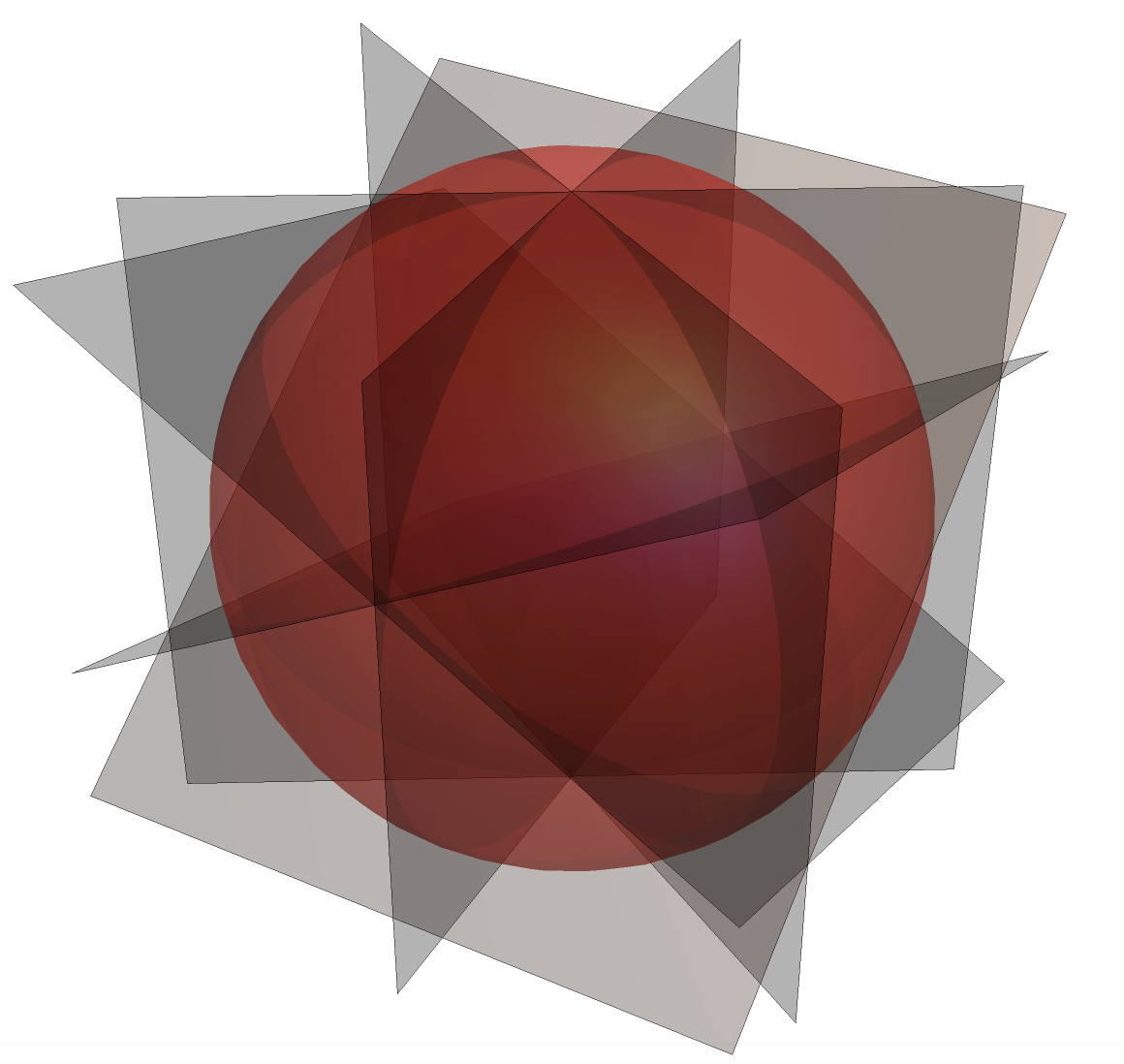 Figure 1
 Figure 2
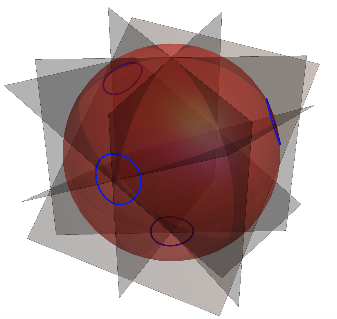 Figure 3
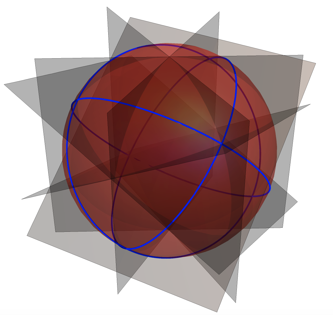 Figure 4
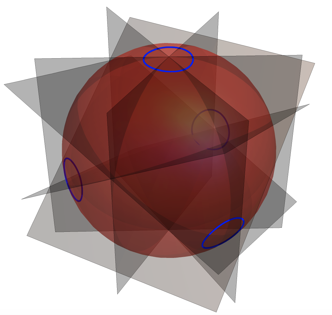 Figure 5
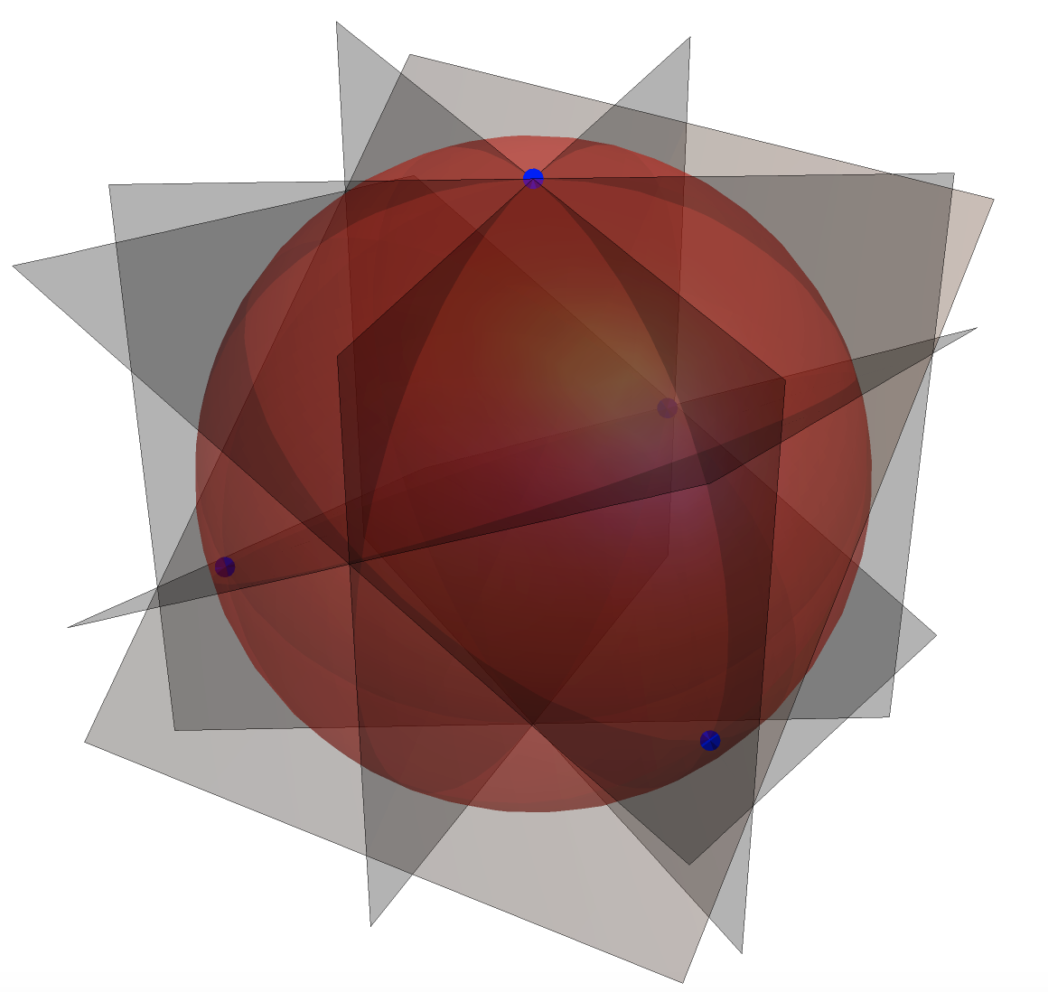 Figure 6
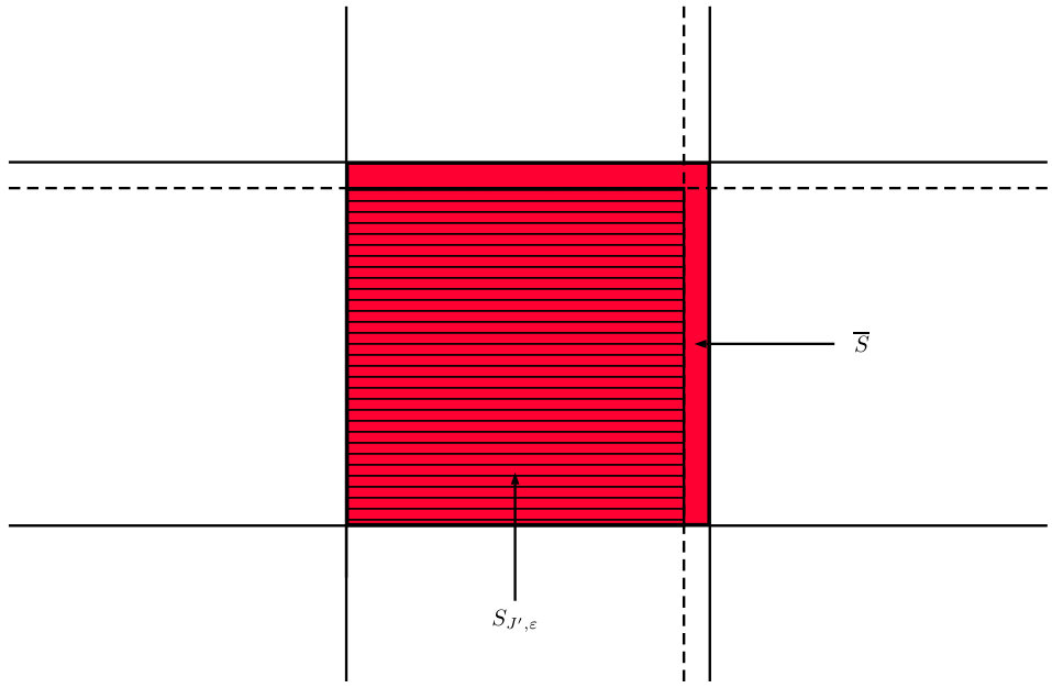 Figure 7
Peer Reviews
No public reviews on file for this paper yet. If you reviewed it on a platform where reviews are public (OpenReview, ICLR, NeurIPS, ICML), you can paste yours below so the community can read it here.
Videos
No videos yet. Explain this paper in a talk, walkthrough, or lecture? Add one.
Vandermonde varieties, mirrored spaces, and the cohomology of symmetric semi-algebraic sets
Saugata Basu
Department of Mathematics, Purdue University, West Lafayette, IN 47906, U.S.A.
and
Cordian Riener
Department of Mathematics and Statistics, UiT The Arctic University of Norway, 9037 Tromsø, Norway
Abstract.
Let be a real closed field. We prove that for each fixed , there exists an algorithm that takes as input a quantifier-free first order formula with atoms , where D is an ordered domain contained in , and computes the ranks of the first cohomology groups, of the symmetric semi-algebraic set defined by . The complexity of this algorithm (measured by the number of arithmetic operations in D) is bounded by a polynomial in and (for fixed and ). This result contrasts with the -hardness of the problem of computing just the zero-th Betti number (i.e. the number of semi-algebraically connected components) in the general case for (taking the ordered domain D to be equal to ).
The above algorithmic result is built on new representation theoretic results on the cohomology of symmetric semi-algebraic sets. We prove that the Specht modules corresponding to partitions having long lengths cannot occur in the isotypic decompositions of low dimensional cohomology modules of closed semi-algebraic sets defined by symmetric polynomials having small degrees. This result generalizes prior results obtained by the authors giving restrictions on such partitions in terms of their ranks, and is the key technical tool in the design of the algorithm mentioned in the previous paragraph.
Key words and phrases:
symmetric semi-algebraic sets, isotypic decomposition, Specht module, Betti numbers, mirrored spaces, computational complexity
1991 Mathematics Subject Classification:
Primary 14F25; Secondary 68W30
Basu was partially supported by NSF grants CCF-1618918, DMS-1620271 and CCF-1910441. Riener was supported by TFS grant 17_matte_CR.
Communicated by Peter Bürgisser.
Contents
-
1.2.2 Partitions of length one and cohomology of the orbit space
-
2.1 Symmetric groups as Coxeter groups and properties of Solomon modules
-
5.2 Replacing an arbitrary semi-algebraic set by a closed and bounded one
-
5.5 Algorithm for computing a semi-algebraic description of the pair
-
5.6 Algorithm for computing the the Betti numbers of symmetric semi-algebraic sets
-
A.1 A quick digest of representation theory of finite groups
1. Introduction and Main Results
Throughout the paper we fix a real closed field, which we will denote by (there is no harm in assuming ). We assume familiarity with the basic notions of semi-algebraic geometry [17, 9] – especially, definitions of semi-algebraic sets, their homology and cohomology groups and main properties.
We will use the following notation.
Notation 1** (Betti numbers).**
Let be any semi-algebraic set. We denote by (here and everywhere else in this paper without further mention we only consider cohomology with rational coefficients and we will denote ). It is worth noting that the precise definition of the cohomology groups requires some care if the semi-algebraic set is defined over an arbitrary (possibly non-archimedean) real closed field. For details we refer to [9, Chapter 7, Section 5].
1.1. Background and main algorithmic result
The algorithmic problem of computing Betti numbers of arbitrary semi-algebraic subsets of is a central and extremely well-studied problem in algorithmic semi-algebraic geometry. It has many ramifications, ranging from applications in the theory of computational complexity where it plays the role of ‘generalized counting’ in real models of computation (see [19, 15]), to robot motion planning where the problem of computing the zero-th Betti number (that is the number of connected components) of the free space of a robot which can be modeled as a semi-algebraic set, is a central problem [41, 24]).
It is well-known that the Betti numbers of semi-algebraic subsets of satisfy a singly exponential (in ) upper bound (see for example [9, Theorem 7.38]). The singly exponential dependence on of the bound is moreover unavoidable as shown by the following (key) example.
Example 1** (Key example).**
Let
[TABLE]
Then, for , the set of real zeros, of in consists of semi-algebraically connected components – each of which is semi-algebraically homeomorphic to a small sphere. Thus,
[TABLE]
and both grow exponentially in (for fixed ).
A common belief in algorithmic semi-algebraic geometry is that topological invariants satisfying a certain bound should in fact be computable by algorithms with complexity bounded by roughly the same estimate. From this point of view one expects that there should exist algorithms for computing the Betti numbers of semi-algebraic sets with complexity bounded singly exponentially. Indeed, algorithms for computing the zero-th Betti number (i.e. the number of semi-algebraically connected components) of semi-algebraic sets have been investigated in depth, and nearly optimal algorithms are known for this problem [7, 14]. An algorithm with singly exponential complexity is known for computing the first Betti number of semi-algebraic sets is given in [10], and then extended to the first (for any fixed ) Betti numbers in [3]. The Euler-Poincaré characteristic, which is the alternating sum of the Betti numbers, is easier to compute, and a singly exponential algorithm for computing it is known [2, 8].
While many advances have been made in recent years [3, 4, 10, 20] the best algorithm for computing all the Betti numbers of any given semi-algebraic set still has doubly exponential (in ) complexity, even in the case where the degrees of the defining polynomials are assumed to be bounded by a constant () [41]. The existence of algorithms with singly exponential complexity for computing all the Betti numbers of a given semi-algebraic set is considered to be a major open question in algorithmic semi-algebraic geometry (see the survey [5]).
One important reason why the problem of designing an algorithm for computing the Betti numbers of semi-algebraic sets with singly exponential complexity is open, is that while the Betti numbers of semi-algebraic sets are bounded by a singly exponential function, the best known algorithm for obtaining semi-algebraic triangulation has doubly exponential complexity [41].
Remark 1* (Other models).*
We remark here that by the word ‘algorithm’ in the previous paragraphs we are referring only to algorithms that work correctly for all inputs and whose complexity is uniformly bounded i.e. bounded in terms of the degrees and the number of input polynomials and independent of the actual coefficients of the polynomials. In contrast to this, there has been very exciting recent work where the authors have given algorithms with singly exponential complexity for computing all the Betti numbers of semi-algebraic sets [21, 23, 22]. However, the complexities of these algorithms depend in addition to the degrees and the number of polynomials, also on the ‘condition number’ of the input. The condition number can be infinite if the given input is ill-conditioned. Thus, such algorithms will fail to produce any result on certain inputs. In this paper we will be concerned with exact algorithms that work for all possible inputs.
From the point of view of lower bounds, the problem of computing even the number of connected components (i.e. the zero-th Betti number) of general (not necessarily symmetric) semi-algebraic sets defined by polynomials of degrees bounded by any constant is a PSPACE-hard problem [39], and thus unlikely to have algorithms with polynomially bounded complexity.
In what follows, we will consider the algorithmic problem of computing the Betti numbers of semi-algebraic sets in the presence of an additional important property – namely symmetry.
1.1.1. Brief History
The study of efficient algorithms for computing topological invariants of symmetric semi-algebraic sets has a shorter history than of such algorithms for arbitrary semi-algebraic set. Using the so called ‘degree principle’ proved by Timofte [45] and Riener [40], one can design an algorithm for deciding emptiness of symmetric algebraic sets in defined by symmetric polynomials of degree , having complexity (i.e. polynomial in for fixed ). The algorithmic questions of computing the equivariant Betti numbers (i.e. the dimensions of – see the end of the paragraph for definition), and also the Euler-Poincaré characteristics of symmetric semi-algebraic sets were considered by the authors of the current paper. In [12], an algorithm with polynomially bounded complexity (polynomial in and the number of polynomials used in the definition of , for fixed ) was described for computing all the equivariant Betti numbers of a closed symmetric semi-algebraic set defined by a formula involving at most symmetric polynomials of degree bounded by . Since we consider cohomology with rational coefficients and because is a finite group, there is an isomorphism , and hence this amounts to computing the Betti numbers of the quotient. In [11], an algorithm with polynomially bounded complexity (better than that of the algorithm mentioned above) was given for computing the equivariant as well as the ordinary Euler-Poincaré characteristics of symmetric semi-algebraic sets.
Before continuing further we introduce some useful notation.
1.1.2. Notation
Notation 2** (Zeros).**
For , we denote by the set of zeros of in . More generally, for any finite set , we denote by the set of common zeros of in .
Notation 3** (Realizations, - and -closed semi-algebraic sets).**
For any finite family of polynomials , we call an element , a sign condition on . For any semi-algebraic set , and a sign condition , we denote by the semi-algebraic set defined by
[TABLE]
and call it the realization of on .
More generally, we call any Boolean formula with atoms, , to be a -formula. We call the realization of , namely the semi-algebraic set
[TABLE]
a -semi-algebraic set.
Finally, we call a Boolean formula without negations, and with atoms , where , to be a -closed formula, and we call the realization, , a -closed semi-algebraic set.
Notation 4** (Symmetric polynomials of bounded degrees).**
For all , we will denote by the subspace of the polynomial ring consisting of symmetric polynomials of degree at most .
Definition 1** (Symmetric semi-algebraic sets).**
We say that a semi-algebraic is symmetric if it is stable under the standard action of the symmetric group permuting coordinates.
Since we will discuss complexities of various algorithms we also make precise the notion of complexity that we are going to use.
Definition 2** (Definition of complexity).**
In our algorithms we will usually take as input polynomials with coefficients belonging to an ordered domain (say D). By complexity of an algorithm we will mean the number of arithmetic operations and comparisons in the domain D. Since is always a subring of D, this will include operations involving integers. If , then the complexity of our algorithm will agree with the Blum-Shub-Smale notion of real number complexity [16]. In case, , then we are able to deduce the bit-complexity of our algorithms in terms of the bit-sizes of the coefficients of the input polynomials, and this will agree with the classical (Turing) notion of complexity.
We are now in a position to state our main algorithmic result.
1.1.3. Main Algorithmic result
Theorem 1**.**
Let D be an ordered domain contained in a real closed field , and let . There exists an algorithm with takes as input a finite set , and a -formula , and computes the tuple of integers
[TABLE]
The complexity of the algorithm, measured by the number of arithmetic operations in D, is bounded by .
If , and the bit-sizes of the coefficients of the input is bounded by , then the bit-complexity of the algorithm is bounded by
[TABLE]
Remark 2* (Polynomiality).*
Note that the complexity of the algorithm in Theorem 1 is bounded by a polynomial in and for every fixed .
Note that as mentioned previously, the analogous algorithmic problem of computing Betti numbers of general (not necessarily symmetric) semi-algebraic sets defined by polynomials of degree bounded by any fixed constant is a -hard problem for (with the coefficients of the input polynomials belonging to ), and thus unlikely to admit algorithms with polynomially bounded complexity.
1.1.4. New ideas
Several new ideas (compared to previous algorithms for computing Betti numbers of semi-algebraic sets) appear in the design of the algorithm cited in Theorem 1.
We begin by replacing the given set by a closed and bounded one defined by symmetric polynomials satisfying the same degree bound as the input polynomials, and whose cohomology groups are isomorphic to those of the given set up to dimension . The key new idea is to utilize the -module structure of the cohomology groups of this new closed and bounded semi-algebraic set. This reduces the problem of computing the dimensions of the cohomology groups of the original set, to that of computing the multiplicities of the various Specht modules appearing in the cohomology groups (up to dimension ) of the new set. The sought after Betti numbers can then be recovered from these multiplicities.
In order to compute the multiplicities of the various Specht modules, we leverage certain techniques originating in the study of cohomology groups of mirrored spaces [27]. These techniques form the basis of the proofs of our representation theoretic results (Theorems 4 and 5). On the algorithmic front they help us in two ways. Firstly, (in small dimensions) it guarantees that only a polynomially bounded many of the multiplicities to be computed can be non-zero, and this restricts the set of partitions that enters into the computation. Secondly, it allows us to obtain a dimension reduction, reducing the problem of computing the multiplicities for any given closed and bounded semi-algebraic set defined in terms of symmetric polynomials of degrees bounded by , to the problem of computing the Betti numbers of pairs of semi-algebraic subsets, which are not symmetric any more but contained in a much smaller () dimensional space. For the latter problem it suffices to use the standard algorithms mentioned previously. We refer the reader to Section 5.1 for a more detailed outline.
1.2. Representation-theoretic results
A key step in the proof of Theorem 1 as outlined above is the computation of the multiplicities of the Specht modules in the cohomology modules of the given semi-algebraic sets. For this we need to consider the isotypic decomposition of cohomology modules. In the next three subsections (namely, Sections 1.2.1, 1.2.2 and 1.2.3) we provide some background and survey prior results, and state the new results in Section 1.2.4. Finally, in Section 1.2.5 we state a representation-theoretic result about the cohomology of a class of very well-studied symmetric varieties (namely Vandermonde varieties) which plays a key role in the proofs of the main theorems of this paper. This result could also be of independent interest.
1.2.1. Isotypic decomposition of cohomology modules
Despite the worst case exponential behavior of the Betti numbers of symmetric varieties, there is one handle we have on them that makes their behavior tame, at least when the degrees of the defining polynomials are held fixed. The action of the symmetric group on symmetric semi-algebraic sets induces an action on the cohomology spaces , giving the structure of a finite dimensional -module (see Definition 13 in Section A.1). General facts from group representation theory (see Appendix A) then tell us that the -module admits a canonically defined isotypic decomposition into a direct sum of sub--submodules, each of which is a multiple of certain irreducible -modules (see Theorem 9, Section A.1). The irreducible -modules are well studied, and they are in bijection with the finite set of partitions of the number – the module corresponding to the partition will be denoted by in what follows, and is called the Specht module corresponding to (see Definition 22 in Section A.2 for the precise definition of these modules).
Thus the isotypic decomposition of gives a direct sum decomposition
[TABLE]
the non-negative integer is called the multiplicity of in .
The dimension of the Specht module , has a simple expression
[TABLE]
which is sometimes called the hook length formula. These dimensions could be exponentially big even for relatively simple partitions (say the partition for even ). Thus, knowing the multiplicities , allows one to compute the dimension of , and thus the Betti numbers of . However, note that the number of partitions of is exponentially large (due to a result of Erdős and Lehner [28]). Thus, this method is at best of exponential complexity, unless we can restrict a priori the number of partitions to consider (i.e. those that are allowed to appear in the isotypic decomposition of the cohomology modules of symmetric semi-algebraic sets that we are considering).
In order to compute the multiplicities efficiently, we prove new quantitative results on the representations of the symmetric group that can appear as cohomology modules of the symmetric semi-algebraic sets under consideration. These results might be of independent interest. In order to relate the new results with prior work and to put them in context, we first survey some known results in the next two sections.
1.2.2. Partitions of length one and cohomology of the orbit space
The partition having length one plays a special role. The corresponding Specht-module is the one dimensional trivial representation of (we also denote it by ), and the isotypic component of corresponding to the partition is thus isomorphic to the fixed part of , which in turn is isomorphic to (see [13] for details and subtleties regarding these isomorphisms). We obtain that the multiplicity of in the cohomology module gives the -th Betti number, . Thus, the problem of computing the dimension of the cohomology of the quotient (or equivalently the space of orbits) is a special case of computing a multiplicity of a particular Specht-module in . We examine this case closely in the next subsection.
It is clear that even in the presence of symmetry the Betti numbers of semi-algebraic sets can be exponentially large (cf. Example 1). However, if in Example 1 we set , and consider the orbits of the action of the symmetric group on the real algebraic set defined in Example 1, then the number of orbits of this action equals the zero-th Betti number of the quotient . (Note that for any symmetric semi-algebraic set the corresponding orbit space can be constructed as the image of a polynomial map and thus is again semi-algebraic [18, 38]).
It is not too difficult to see that the orbit of a point is determined by the tuple , where .
Thus, the number of orbits of , and thus the sum of the Betti numbers of the quotient equals , which satisfies the inequalities
[TABLE]
where are constants that depend only on .
Note that
[TABLE]
and (cf. Eqn. (1.1)). Moreover, notice that unlike the Betti numbers of itself, the Betti numbers of the quotient, , are bounded by a polynomial in (for fixed ), and moreover the degree of this polynomial is .
In fact, the following general theorem is proved in [12, Theorem 6] of which the phenomenon exhibited above is a particular case.
Theorem 2**.**
[12*]**
Let be a -closed semi-algebraic set, where*
[TABLE]
* and . Then,*
[TABLE]
The following theorem which also appears in [12, Theorem 10] indicates that the orbit-space case is markedly different from the general (non-symmetric) case from the point of view of algorithmic complexity as well.
Theorem 3**.**
[12*]**
For every fixed , there exists an algorithm that takes as input a -closed formula , where , and outputs , where . The complexity of this algorithm is bounded by .*
Notice that for fixed the complexity of the algorithm in Theorem 3 is polynomial in and . Taken together, Theorems 2 and 3 show a dramatic reduction of complexity – both topological and algorithmic – when passing from a symmetric variety to its orbit space.
1.2.3. General partitions
We now return to the study of the cohomology of a symmetric semi-algebraic set itself – rather than its quotient. Before proceeding further it is useful to go back to our key example (Example 1).
Example 2** (Key example continued with ).**
We set the degree and in the polynomial in Example 1, and denote and .
We now describe the isotypic decomposition of . The details of this computation appear in [13] and are omitted here. In dimension [math] we get:
[TABLE]
where
[TABLE]
Notice that for , by the hook-length formula we have,
[TABLE]
Note that since , we obtain as a consequence (from (1.4) and (1.6)) the slightly non-obvious identity
[TABLE]
Notice that Eqns. (1.3), (1.4), and (1.7) illustrate the phenomenon of how an exponentially large dimensional cohomology group is built out of a relatively small (i.e. polynomially bounded) number of pieces – each of which is a multiple (with polynomially bounded multiplicity) of certain Specht modules.
The decomposition of the cohomology modules of a closed semi-algebraic set defined by symmetric polynomials having degrees at most into isotypic components was studied in [13], where several results were proved. The first important result was a severe restriction on the partitions that are allowed to appear in the isotypic decomposition of the cohomology – which cuts down the possibilities for the allowed partitions from exponential to polynomial (for fixed ). More precisely, it is shown in [13] that with the same hypothesis as Theorem 2,
[TABLE]
where is the size of the largest square (also referred to as the ‘Durfee square’ of the partition) that can fit inside the Young diagram (cf. Definition 20 in Section A.2) of the partition . For every fixed , the number of partitions of satisfying the condition is polynomially bounded in (unlike the total number of partitions which grows exponentially).
The second key result obtained in [13] is a polynomial bound (again for fixed ) on the multiplicities occurring in the isotypic decomposition of . Taken together – the polynomiality of the number of allowed partitions, and the polynomiality of their multiplicities – gives rise to the hope (via the ‘common belief’ alluded to before), that the Betti numbers of symmetric semi-algebraic sets defined by symmetric polynomials of degrees bounded by a constant, could be computed with polynomially bounded complexity.
1.2.4. New representation-theoretic results
We now describe the new representation theoretic results that makes it possible to partially realize the ‘hope’ expressed above. We obtain restrictions on the Specht modules, , that are allowed to appear depending on and , as well as the dimension (or the degree) of the cohomology group under consideration. These restrictions are of two kinds. Firstly, we prove that when is fixed, the Specht modules corresponding to partitions having long lengths cannot occur in the isotypic decompositions of small dimensional cohomology modules of semi-algebraic sets defined by symmetric polynomials of degrees bounded by . Secondly, we prove that the Specht modules corresponding to partitions having short lengths cannot occur in the isotypic decompositions of the high dimensional cohomology modules of semi-algebraic sets defined by symmetric polynomials of degrees bounded by .
Notation 5**.**
Recall that for any symmetric semi-algebraic subset and , we denote by the multiplicity of in the isotypic decomposition of , i.e., . We will denote
[TABLE]
We prove the following theorem. The notation used in the theorems in this section is mostly standard; but readers unfamiliar with them should consult Appendix A.
Theorem 4**.**
Let , and be a -closed semi-algebraic set with . Then, for all :
- (a)
[TABLE]
or equivalently,
[TABLE] 2. (b)
[TABLE]
or equivalently,
[TABLE]
Part (a) of Theorem 4 can be read as saying that for any fixed , and a -semi-algebraic set with ,
[TABLE]
Similarly, Part (b) of Theorem 4 can be read as saying that
[TABLE]
The following analysis of the cohomology modules of the key example (Example 1) shows that up to a multiplicative constant the bounds stated in Theorem 4 on and for are tight.
Example 3** (Key example continued).**
For , and , consider the real algebraic set defined in Example 1. Recall that for , consists of disjoint topological spheres, each sphere infinitesimally close (as a function of ) to one of the points .
Thus, for , , and and . We now describe the isotypic decomposition of for , and .
In what follows, for , we denote by the partition of obtained by permuting the ’s so that they are in non-increasing order.
It is shown in [13] that
[TABLE]
where denotes the partial order often referred to as the dominance order on the set of partitions of , and are the Kostka numbers (see [25] for definitions).
It is clear from (1.9) that there exists with , such that
[TABLE]
which shows that the restriction, (in the case ) in Part (a) of Theorem 4 is tight up to a multiplicative factor.
It follows from the -equivariant Poincaré duality (see for example [13, Theorem 3.23]), that
[TABLE]
This shows that there exists with , such that
[TABLE]
So the restriction, (in the case ) in the Part (b) of Theorem 4 is also tight up to a multiplicative factor.
1.2.5. Role played by Vandermonde varieties
The proof of Theorem 4 stated in the previous section depends crucially on a similar restriction theorem for a class of symmetric semi-algebraic sets which are particularly simple to define – namely, Vandermonde varieties. Vandermonde varieties have been studied widely in a series of papers by Arnold [1], Giventhal [30], Kostov [32] amongst others, mainly from a topological point of view. The representation-theoretic results we prove in this paper on their cohomology modules are new and might be of independent interest. The restrictions on the -module structure for Vandermonde varieties, produce via an application of an argument involving the (equivariant) Leray spectral sequence, similar (slightly looser) restrictions on the cohomology modules of arbitrary symmetric semi-algebraic sets defined by quantifier-free formula involving qualities and inequalities of symmetric polynomials of degrees bounded by (cf. Theorem 4).
The intersections of the level sets of the first (weighted) Newton power sums in for some have been called Vandermonde varieties by Arnold [1] and Giventhal [30], who studied their topological properties in detail. When the weights are all equal the Vandermonde varieties are also symmetric with respect to the standard action (by permuting coordinates) of the symmetric group , and thus the cohomology groups of the Vandermonde varieties acquire the structure of finite dimensional -modules.
Remark 3*.*
If one replaces in the definition of Vandermonde varieties, the Newton power sums with any other set of generators of the ring of -invariant polynomials (for example the elementary symmetric polynomials), the intersection of the level sets of the generators of degree at most give the same class of real varieties. Indeed, Vandermonde varieties can be defined as level sets of the first generators of the invariant ring of any finite reflection group, and many results and techniques introduced in the current paper extend to more general reflection groups. However, the case of the symmetric group is the most important from the point of view of applications, and we restrict ourselves to this special case in this paper.
In their foundational work on the topic, Arnold [1], Giventhal [30] and Kostov [32], proved that the intersection of a symmetric Vandermonde variety with the Weyl chamber in , defined by the inequalities is contractible if non-empty, which in turn implies that the quotient space of a symmetric Vandermonde variety is contractible if non-empty.
As a first step towards proving Theorem 4 we study the -module structure of the cohomology groups of symmetric Vandermonde varieties themselves (not just their quotient space). We prove the following theorem.
Theorem 5**.**
Let , , and let denote the Vandermonde variety defined by , where . Then, for all :
- (a)
[TABLE]
or equivalently,
[TABLE] 2. (b)
[TABLE]
or equivalently,
[TABLE]
Remark 4* (Cases ).*
The case is omitted in Theorem 5. Indeed, Part (a) is not true as stated in the case . In this case, is the hyperplane defined by the equation
[TABLE]
and is -equivariantly contractible to the point . Hence
[TABLE]
(recall that the Specht module for equal to the trivial partition is isomorphic to the one-dimensional trivial representation). It follows that for ,
[TABLE]
but
[TABLE]
which violates (1.11).
On the other hand, the case already indicates that the bounds in Theorem 5 is sharp.
If and , the Vandermonde variety is the defined by the equation
[TABLE]
and can be empty, a point, or semi-algebraically homeomorphic to a sphere of dimension (depending on whether is , or , respectively). In the last case (i.e. when ):
[TABLE]
(see Subsection 3.2.1 below for a proof).
It follows that for and ,
[TABLE]
and
[TABLE]
1.2.6. Improvements over prior work
Theorems 4 and 5 are improvements over prior results in [13] (Theorem 2.5, Part (1)) having similar flavor in several different ways.
Firstly, the restrictions (cf. (1.8)) on partitions given in [13, Theorem 2.5] are in terms of upper bounds on their ranks rather than their lengths. While the length of a partition is an upper bound on its rank, a partition having small rank can be arbitrarily long. For example, the partition has rank , but its length is clearly the maximum possible, namely .
Secondly, the restrictions in [13, Theorem 2.5] do not take into consideration the dimension (or the degree) of the cohomology groups under consideration. In contrast, the restrictions on the partitions given in Theorems 4 and 5 in the current paper, do depend in a strong manner on the dimension (or the degree) of the cohomology group. As a result in small dimensions, we obtain that only the partitions with a small length can appear unlike the restrictions obtained in [13], where there were no non-trivial restriction on the length. The restriction on the length is a key ingredient in the algorithmic result obtained in this paper.
The results of the current paper depend on:
- (a)
results from the cohomological study of mirrored spaces due to Davis [26] and Solomon [43], 2. (b)
fundamental results on Vandermonde varieties due to Arnold [1], Giventhal [30] and Kostov [32], and 3. (c)
a careful topological analysis of certain regular cell complexes that arise in the process of combining these results.
In contrast, the proofs of the results in [13] are based essentially on equivariant Morse theory which plays no role in the current paper. The reader who is curious about the interplay of results coming from different areas and how they combine together in the study of Vandermonde varieties, can skip forward to Examples 3.2.1 and 3.2.2 where the examples of Vandermonde varieties of degree in , , and that of degree in are worked out in full detail.
The rest of the paper is dedicated to the proofs of Theorems 1, 4, and 5. In Section 2, we prove a few preliminary results on the Solomon decomposition of the cohomology groups of mirrored spaces that play an important role in the rest of the paper. We introduce all necessary background material referring the reader to Appendix A for the more basic material on representation theory of finite groups and of the symmetric groups in particular that we utilize. In Section 3 we give outlines of the proofs of Theorems 4 and 5, and also describe two important examples illustrating the main steps. In Section 4, we give the proofs of Theorems 4 and 5. In Section 5 we give the proof of Theorem 1 after introducing the necessary preliminary results.
2. Solomon modules and mirrored spaces
This section is divided into two subsections. In the first subsection (Subsection 2.1) we discuss the representation theory of the symmetric groups by viewing them as examples of finite Coxeter groups drawing on the work of Solomon [43]. In particular, we show how to obtain the isotypic decomposition of the Solomon modules (which are certain representations of symmetric groups that we define in this section), and prove certain quantitative statements about them that are key to the proofs of the main theorems of the paper. These results (namely, Propositions 2 and 3 and Corollary 1) are the only results from this section that are used later in the paper.
In the second subsection (Subsection 2.2) we introduce mirrored spaces and discuss a key theorem (cf. Theorem 7) giving a formula for the cohomology of a mirrored space in terms of certain Solomon modules. This theorem plays a central role in the proof of Theorem 5.
2.1. Symmetric groups as Coxeter groups and
properties of Solomon modules
Recall that a Coxeter pair , consists of a group and a set of generators, , of each having order , and numbers such that .
Our main example of a Coxeter groups will be the symmetric group considered as a Coxeter group with the set of Coxeter generators, (here denotes the permutation of which exchanges and keeping all other elements fixed).
We will need the notion of length of an element of a Coxeter group.
Notation 6** (Length of an element of ).**
Given Coxeter pair , with , and an element , we call to be the length of (denoted ), if is minimal amongst all such expressions for .
Example 4**.**
If , the lengths of the various elements of viewed as permutations are displayed below.
[TABLE]
Following the same notation as in [27], for , we denote by the subgroup of generated by , and let
[TABLE]
We will write . For , let
[TABLE]
For , we denote (following [43])
[TABLE]
2.1.1. Algebras, tensor products and representations
Let be a group and be the group algebra of . A left ideal is then a (left) -module. Now let be two Coxeter groups, and be their group algebras. Then, the tensor product is again an algebra, where the multiplication is defined by . Moreover, is isomorphic as an -algebra to , where the isomorphism is given by
[TABLE]
If are subgroups of , such that is the (internal) direct product of , then the isomorphism,
[TABLE]
is given by .
Finally, if is a left ideal of , and a left ideal of , then is a left ideal of the algebra . If we denote by (resp. ) the -representation (resp. -representation) corresponding to (resp. ), then we will denote by the -representation corresponding to . We will need later the following proposition.
Proposition 1**.**
Let , and . Let , such that , and
[TABLE]
Then,
[TABLE]
Proof.
Let , , and . Observe first that the elements of commute with the elements of , , and . Hence it follows that is isomorphic to the direct product of the subgroups and . In particular, every element can be written uniquely as
[TABLE]
with and . Moreover,
[TABLE]
It follows from (2.3) that (resp. ) is the -representation (resp. -representation) corresponding to the left ideal of (resp. of ).
Moreover, there is an isomorphism of -algebras (see (2.4)) , defined by . It suffices to prove that carries the left ideal of surjectively to the left ideal of .
Since, is spanned by the elements it suffices to prove that
[TABLE]
for every .
Using the fact that every element can be written uniquely as with and , with
[TABLE]
[TABLE]
Hence
[TABLE]
Now can be written (uniquely) as with and , and hence
[TABLE]
This finishes the proof. ∎
Notation 7** (Solomon modules).**
For ease of notation we will denote the representation by . We will call the Solomon module indexed by .
Remark 5*.*
The Solomon modules may be understood as analogs of Specht modules (cf. Definition 22), but defined in terms of MacMahon’s tableau [34, Vol 1, Chapter 1, Sect IV, 129.] rather than Young’s tableau (cf. Definition 21) where the role of partitions is replaced by that of compositions (cf. Notation 20). Unlike the Specht modules, the representations need not be irreducible (see Example 6). But we are able to obtain a necessary condition for a Specht module to appear with positive multiplicity in using a recursive formula due to Solomon [43, Corollary 3.2] (cf. Proposition 3 below).
Remark 6*.*
As remarked above the representations need not be irreducible in general. However, it is easy to see from (2.3), Notation 7 and Definition 22, that in the following two special cases, they are indeed irreducible.
[TABLE]
Another easy consequence of (2.3) is
[TABLE]
2.1.2. Relation between Solomon modules and Specht modules
We next prove a recursive formula for computing the multiplicities of Specht modules in the Solomon modules (Proposition 2 and Corollary 1). We also prove a condition (in terms of and the cardinality of ) on partitions which needs to be satisfied for to hold (Proposition 3).
Proposition 2**.**
Let , , and
[TABLE]
Then,
[TABLE]
Proof.
Let
[TABLE]
Notice that
[TABLE]
Claim 1**.**
[TABLE]
Proof of Claim 1.
Observe that it follows from the definitions of that
[TABLE]
and
[TABLE]
Now,
[TABLE]
using Proposition 1. Finally, from the fact that , , and , we have
[TABLE]
and
[TABLE]
This finishes the proof of the claim. ∎
Claim 2**.**
[TABLE]
Proof of Claim 2.
Observe that
[TABLE]
It follows directly from [43, Corollarly 3.2] that
[TABLE]
which completes the proof of the claim. ∎
The proposition now follows directly from Claims 1 and 2. ∎
The following corollary of Proposition 2 will be useful in designing an algorithm for computing isotypic decomposition of the Solomon modules .
Corollary 1**.**
Let , , and
[TABLE]
Then, for any ,
[TABLE]
Proof.
Follows directly from Proposition 2 and Schur’s Lemma (Lemma 5 in the Appendix). ∎
Before proceeding further we recall a classical formula – namely Pieri’s rule.
Notation 8**.**
For , and , we denote by the set consisting of partitions either of the form satisfying:
[TABLE]
and
[TABLE]
or of the form satisfying:
[TABLE]
and
[TABLE]
In other words , if and only if and the Young diagram corresponding to is obtained from that of by adding boxes, such that no two boxes are added in the same column.
Example 5**.**
For example,
[TABLE]
The significance of the set is encapsulated in the following lemma. With the same notation as in Notation 8:
Lemma 1** (Pieri’s rule).**
- (a)
[TABLE] 2. (b)
For each , .
Proof.
Part (a) is just Pieri’s rule (see for instance [35, Page 109]). Part (b) is obvious from definition of (cf. Notation 8). ∎
The following lemma in conjunction with Lemma 1 will be used in the complexity analysis of Algorithm 1.
Lemma 2**.**
Let , , and . Then,
[TABLE]
Proof.
Obvious from Eqns. (2.13), (2.14), (2.15) and (2.16). ∎
Remark 7*.*
Corollary 1 gives us an inductive method (using double induction on and ) for obtaining the isotypic decomposition of the Solomon modules , since the Solomon modules that appear on the right hand side of (2.12) are either of a strictly smaller symmetric group since , or the Solomon module of but with respect to a smaller set of Coxeter elements (since ). Moreover, the isotypic decomposition of the representation can be computed from that of using Part (a) of Lemma 1 (Pieri’s rule).
For the base cases notice that is isomorphic to the trivial representation, if , and for , the is again the trivial representation (the only that can appear is the empty set).
This algorithm for computing the isotypic decomposition of using the inductive method sketched above is formally described in Algorithm 1 in Section 5, where we analyze the complexity of this algorithm as well. We illustrate the method here by giving an example.
Example 6**.**
Let and . We will use Proposition 2 to obtain the isotypic decomposition of . In this example . So applying Proposition 2 we obtain
[TABLE]
Now (using (2.7))
[TABLE]
Using Part (a) of Lemma 1 we get
[TABLE]
In conjunction, (2.17) and (2.18) implies
[TABLE]
whence
[TABLE]
Note that this example also illustrates the fact that the Solomon modules need not be irreducible.
Another important consequence of Proposition 2 that will be important for us is a bound (in terms of the cardinality of alone) on the lengths of the partitions corresponding to the Specht modules that can appear in the isotypic decomposition of . We deduce such a bound in the following proposition.
Proposition 3**.**
Let , . Then, for ,
[TABLE]
Remark 8*.*
Note that the bound in Proposition 3 above is the best possible (cf. Example 6).
Proof of Proposition 3.
We first prove that
[TABLE]
The proof is by a double induction on , and on . Clearly, (2.19) holds for and for all . Also, if (i.e. )
[TABLE]
and (2.19) holds for all .
Now suppose that the proposition is true for all , and for given for all and suppose that .
Observe that for , using the fact that and the induction hypothesis we get that
[TABLE]
Using Part (a) of Lemma 1 for any ,
[TABLE]
[TABLE]
It follows from (2.20), (2.21) and (2.22), that for ,
[TABLE]
The claim in (2.19) now follows from (2.23), Proposition 2 and Schur’s Lemma (Lemma 5 in the Appendix). This finishes the inductive proof of (2.19).
We now prove
[TABLE]
First observe that using (2.9)
[TABLE]
It follows that
[TABLE]
∎
We now introduce a geometric construction (that of a mirrored space) which will play an important role later.
2.2. Mirrored spaces and Weyl chambers
We first recall a definition from [27].
Definition 3** (Mirrored space).**
Given a Coxeter pair (i.e. is a Coxeter group and a set of reflections generating ) a space with a family of closed subspaces is called a mirror structure on [27, Chapter 5.1], and along with the collection is called a mirrored space over .
Given a mirrored space over , there is a classical construction (called ‘The Basic Construction’ in [27, Chapter 5]) of a space with a -action which we define as follows.
Definition 4** (The Basic Construction [33, 46, 48, 26]).**
We define
[TABLE]
where the topology on is the product topology, with given the discrete topology, and the equivalence relation is defined by
[TABLE]
with
[TABLE]
and the subgroup of generated by .
The group acts on by (where denotes the equivalence class of under the relation ).
For a mirrored space over , the cohomology groups, , gets a structure of a -module from the -action on , and . The cohomology groups of are studied in [27] in the case where is a finite CW-complex, however in this paper we are concerned with mirrored spaces which are semi-algebraic.
2.2.1. Semi-algebraic mirrored spaces
Definition 5**.**
We will call a mirrored space over , to be a semi-algebraic mirrored space over , if and each are semi-algebraic sets.
Remark 9*.*
First observe that for a finite group , and a semi-algebraic set , is again a semi-algebraic set. Moreover, if is closed and bounded, so is , and the quotient is also semi-algebraic, since the quotient of a semi-algebraic set by a proper semi-algebraic equivalence relation is semi-algebraic ([47, page 166]).
Note also that every closed and bounded semi-algebraic set is semi-algebraically homeomorphic to the geometric realization over of a finite simplicial complex (see for example [9, Chapter 5]). More generally, if is a semi-algebraic mirrored space, with closed and bounded, then there exists a finite simplicial complex and subcomplexes , and a semi-algebraic homeomorphism , which restricts to homeomorphisms .
Moreover, for any subset , the cohomology groups of (resp. pairs ) are isomorphic to the simplicial cohomology groups of the simplicial complex (resp. pairs ) (see [9, Chapter 6]).
In view of Remark 9 the following theorem stated in [27] for finite CW-complexes remain true for semi-algebraic mirrored space with closed and bounded. We state the theorem in the special case where which is the only case of interest to us in this paper.
Theorem 6**.**
[27*, Theorem 15.4.3]**
Let , and a semi-algebraic mirrored space over , and closed and bounded. Then,*
[TABLE]
where for each ,
[TABLE]
2.2.2. Weyl chambers
The semi-algebraic mirrored spaces that we will be interested in are of a special type. In order to introduce them we first need a few more definitions.
Notation 9**.**
We denote by the cone defined by , and by the interior of (i.e. the cone defined by ).
Notation 10**.**
For , we denote by the set of integer tuples
[TABLE]
Definition 6**.**
For , and , we denote by the subset of defined by,
[TABLE]
and denote by the subset of defined by
[TABLE]
We denote by the subspace defined by
[TABLE]
which is the linear hull of .
Notation 11**.**
For , we denote by the face of defined by . More generally, for , we denote:
[TABLE]
We also define implicitly by the equation
[TABLE]
Notation 12**.**
Finally, for any semi-algebraic set , , we set
[TABLE]
For any semi-algebraic subset , we will denote
[TABLE]
and we will for convenience of notation write (respectively, ), in place of (respectively, ).
Now suppose that is a closed and bounded symmetric semi-algebraic subset of , then (using Notation 12) . Then, along with the tuple of closed semi-algebraic subsets (cf. Notation 11) is a semi-algebraic mirrored space over .
It follows immediately from Definition 4 that
Proposition 4**.**
The semi-algebraic set is semi-algebraically homeomorphic to .
Proof.
It is a simple exercise to verify that the map
[TABLE]
is a semi-algebraic homeomorphism . ∎
Proposition 4 in conjunction with Theorem 6 yields the following result that we will use later in the paper. This is the only result from this subsection that we will need in the rest of the paper.
Theorem 7**.**
Let be a closed and bounded symmetric semi-algebraic subset of . Then,
[TABLE]
∎
3. Outline of our method and two important examples
3.1. Outline of the proofs of Theorems 4 and 5
We first observe that symmetric semi-algebraic subsets , defined in terms of equalities and inequalities of symmetric polynomials of degree at most , admits a map to (by the first Newton power sum polynomials restricted to ), whose fibers are Vandermonde varieties. Moreover the action of keeps the fibers stable, and thus the action of on also induces an action on the Leray spectral sequence of this map. As a result in order to prove the vanishing of certain irreducible -modules, it suffices to prove this vanishing for Vandermonde varieties. The Vandermonde varieties are well studied and have nice topological and geometric properties. For us the most important property implicit in the work of Arnold, Giventhal and Kostov is that the intersection of a Vandermonde variety with a Weyl chamber in is either a point or a regular cell of the dimension of the variety. Moreover, the structure of the boundary of (in case is a regular cell) is well understood in terms of the combinatorics of the faces of with which has a non-empty intersection.
Applying Theorem 7 to our situation we obtain that the cohomology groups of are isomorphic to direct sums of tensor products of the Solomon modules , indexed by subsets , and the cohomology groups of the pairs , where as before
[TABLE]
Recall now that by Proposition 3 only those Specht modules can appear in whose number of rows is bounded by (and a similar restriction in terms of the number of columns).
One final ingredient is the observation that in the case when has the expected dimension , then the intersection of with the various faces of , induces a structure of a regular cell complex, and the boundary of is then semi-algebraically homeomorphic to the -dimensional sphere, and the intersection of with the various , gives an acyclic covering of the boundary of having cardinality at most . This implies via an argument using the nerve lemma and Alexander duality that the cohomology groups must vanish if is large compared to the cardinality of and also a dual statement (cf. Proposition 6).
Putting these together we obtain our theorem on the vanishing of certain multiplicities for Vandermonde varieties (cf. Theorem 5). Theorem 4 is then a consequence of Theorem 5 and an argument involving (an equivariant version of) the Leray spectral sequence.
Finally, the restriction result that we prove also allows us, via the Solomon-Davis formula alluded to above, and some additional ingredients (see the outline in Section 5.1) including certain standard algorithms from semi-algebraic geometry, to effectively compute the Betti numbers , for any fixed with complexity which is polynomial in the number of variables and the number of polynomials. Here we are assuming that the degrees of the input polynomials are also bounded by a constant.
We will now proceed to describe two important examples, whose analysis already exposes the central ideas behind the proofs of the main theorems.
We first introduce some more notation.
Notation 13**.**
For every , and we denote
[TABLE]
and for every , and we denote by the continuous map defined by
[TABLE]
where .
Finally, we denote by
[TABLE]
the restriction of to .
If , then we will denote by the polynomial (the -th Newton sum polynomial), and by (respectively, ) the map (respectively, ).
For every , , and , we will denote by
[TABLE]
If , then we just denote by , and by .
We are now ready to discuss the promised examples.
3.2. Examples
3.2.1. Example with and .
We first consider the case for , which has already being alluded to in Remark 4. Recall that in this case, the Vandermonde variety is defined by the equation
[TABLE]
and is empty, a point, or a semi-algebraically homeomorphic to a sphere of dimension (depending on whether is , or , respectively).
The first two cases are trivial. In the last case, is a closed disk of dimension , and has a non-empty intersection with all the faces of the Weyl chamber . (See Figure 1(a) for the case , where is one of the triangles on the two-dimensional sphere equal to . Notice that in this case meets all the three faces of the Weyl chamber .)
It follows that in this case
[TABLE]
The -module structure of stated in (4) in Remark 4 now follows from (3.2.1), (2.7), (2.8),and Theorem 7.
3.2.2. Example of
We now study the cohomology of the symmetric Vandermonde varieties (curves) , as -modules, for various .
In this case the Weyl chamber has three faces corresponding to the compositions , and . In terms of the Coxeter elements , , and , these faces correspond to , , and respectively. In other words, using the notation introduced in (2.26),
[TABLE]
Also, note that
[TABLE]
We first need a preliminary calculation. Observe that
[TABLE]
From this we deduce that
[TABLE]
and using (2.9) that,
[TABLE]
Returning to the study of topology of the curve , there are five different cases possible depending on the configuration of the curve inside . Recall (cf. Notation 13) that we denote .
- Case 1.
The Vandermonde variety is empty: in this case , and . 2. Case 2.
The Vandermonde variety is singular and is non-empty: in this case, is a point which must necessarily belong to the face labeled by of . Thus, belongs to all non-zero faces of , and is a minimum value of on . (This preceding fact follows from Theorem 8 stated later.)
In this case (using Notation 12)
[TABLE]
This implies that
[TABLE]
It follows that (using the Eqn. (A.2)). Clearly, in this case. 3. Case 3.
The Vandermonde variety is non-empty and non-singular. Lets fix such that is non-empty and non-singular. In this case, is a sphere which is depicted in Figure 1(a).
The hyperplanes (shown in grey) in Figure 1(a) cutting out the triangles on the sphere are the walls of the various Weyl chambers. Notice that there are vertices in the arrangement of great circles on the sphere, of them incident on circles and the remaining incident on circles. There are several sub-cases to consider. The (non-empty) sub-cases are depicted in Figures 1(b), 1(c), 1(d) and 1(e) ( is shown in blue).
It follows from Theorem 8 that there exist,
[TABLE]
with
[TABLE]
giving a partition of into points and open intervals (more precisely, three points and four open intervals) such that the Vandermonde variety can be characterized topologically by which element of the partition belongs to.
- 3a.
: In this case, ; 2. 3b.
: In this case, is non-empty and singular, and coincides with of the vertices of degree , and is a point which must necessarily belong to the face labeled by (cf. Theorem 8). In this case
[TABLE]
if
[TABLE]
(since in these cases ), and
[TABLE]
in the case
[TABLE]
This implies that
[TABLE]
It follows that
[TABLE]
(using (A.2) to derive ). Clearly, in this case. 3. 3c.
: In this case is a non-singular curve, and intersects the faces labeled by and corresponding to Coxeter elements and respectively.
In this case,
[TABLE]
if
[TABLE]
and
[TABLE]
if
[TABLE]
This implies that
[TABLE]
In dimension one we have,
[TABLE]
if
[TABLE]
and
[TABLE]
if
[TABLE]
This implies that
[TABLE]
It follows that
[TABLE]
and
[TABLE] 4. 3d.
: In this case, the Vandermonde variety is of dimension but has singularities, and intersects the faces labeled by and (the intersection with the face labeled are the singular points of ). Thus, intersects the faces labeled by Coxeter elements and .
In this case,
[TABLE]
if
[TABLE]
and
[TABLE]
if
[TABLE]
This implies that
[TABLE]
In dimension one we have,
[TABLE]
if
[TABLE]
and
[TABLE]
if
[TABLE]
This implies that
[TABLE]
It follows that
[TABLE]
and
[TABLE]
This last equation can be verified directly by hand noting that has the structure of a connected graph containing vertices (the singular points consisting of the orbit of the point ), and the degree of each vertex is . Thus the graph has edges, and hence
[TABLE]
and thus,
[TABLE] 5. 3e.
: In this case, is a non-singular curve, and intersects the faces labeled by and corresponding to Coxeter elements and respectively. The isotypic decomposition of in this case is identical to the Case (3c) and is omitted. 6. 3f.
: In this case, is non-empty and singular, and coincides with other (compared to Case (3b)) of the vertices of degree . In this case, is a point which must necessarily belong to the face labeled by . The isotypic decomposition of in this case is identical to the Case (3b) and is omitted. 7. 3g.
: In this case, is again empty.
Notice, that the Specht module does not appear with positive multiplicity in , in the above analysis. Using an equivariant Leray spectral sequence argument (cf. proof of Theorem 4) we can deduce from this fact the following ‘toy’ theorem (which is not directly deducible from the statement of Theorem 4):
Theorem**.**
If is a -semi-algebraic set, for , then
[TABLE]
Proof.
See proof of Theorem 4 and the preceding remark. ∎
Remark 10*.*
Note that it follows from the analysis in Example 3.2.2 that
[TABLE]
while the Part (a) of Theorem 5 provides the upper bounds:
[TABLE]
Thus, Example 3.2.2 is in agreement with Theorem 5.
We now return to the proofs of the main theorems.
4. Proofs of Theorems 4 and 5
We first need a few preliminary results.
4.1. Preliminary Results
We start by recalling a standard definition.
Definition 7**.**
We say that a semi-algebraic set is a semi-algebraic regular cell of dimension , if the pair is semi-algebraically homeomorphic to where denotes the unit ball in .
Remark 11* (Monotonicity and regularity of semi-algebraic sets).*
We will prove in Proposition 5 that the intersections of weighted Vandermonde varieties with the interior of is a semi-algebraic regular cell of dimension , if the dimension of the variety is equal to , and this property will play an important role later in the paper (see Lemma 3 and Proposition 6). To prove that a given semi-algebraic set is a semi-algebraic regular cell is often not easy. In order to overcome this difficulty, a stronger notion, that of a monotone cell, was introduced in [6]. The property that a semi-algebraic set is a monotone cell is much easier to check. We do not reproduce the definition of a monotone cell here but refer the reader to [6, Theorem 9] for one of the several equivalent definitions which is the easiest to check for the sets . Finally, the main result (Theorem 6) in [6] states that a semi-algebraic set which is a monotone cell is a semi-algebraic regular cell, which is what we will use in the proof of Proposition 5.
The following proposition which has been referred to before, and which describes the topological structure of the intersection of a general Vandermonde variety with a Weyl chamber, is a key topological ingredient in our proofs.
Proposition 5**.**
For every , , and , is either empty, a point, or semi-algebraically homeomorphic a semi-algebraic regular cell of dimension .
Proof.
Suppose that is not empty. Let and suppose that is a regular point of the intersection of the Vandermonde variety with the linear subspace (i.e. the linear hull of the face ) for some . Then, is a regular point of , and .
We next prove that if , then must be a point. Indeed, if , but , then by the above observation and [1, Theorem 5], , with , and moreover . Moreover, in this case must be an isolated point of , since any neighborhood of in , unless equal to just itself, will contain some regular point of the intersection of with with , and this would imply that . But on the other hand we know that is contractible [32, Theorem 1.1]. This proves that in this case , and hence if , is a point.
So we might suppose that
[TABLE]
In this case , and using [1, Theorem 5] is non-singular of dimension . Now using [32, Corollary 2.2], and [6, Theorem 9] we deduce that is a monotone cell (see [6] for the definition of a monotone cell). This implies using [6, Theorem 13] that is a regular cell. In conjunction with (4.1) this implies that is semi-algebraically homeomorphic to the closure of a regular cell, and the boundary of is semi-algebraically homeomorphic to the sphere \mbox{{\bf S}}^{k-d-1}. ∎
Remark 12*.*
Using Proposition 5 again on the intersection of with the faces of we get that if is not empty or a point, then its boundary is a regular cell complex (homeomorphic to \mbox{{\bf S}}^{k-d-1}).
Definition 8**.**
Let be a closed and bounded semi-algebraic set and be a finite set of closed semi-algebraic subsets of . We say that , where is a finite set, is a closed Leray cover of if satisfies:
- (a)
; 2. (b)
for each subset , is empty or semi-algebraically contractible.
We say that is a regular closed Leray cover if in addition for each subset , is empty or the closure of a regular semi-algebraic cell.
Notation 14** (Nerve complex associated to a closed Leray cover).**
Given a closed Leray cover with , we will denote by the simplicial complex whose set of -dimensional simplices are given by
[TABLE]
We need the following technical lemma in the proof of Proposition 6 which plays an important role in the proof of Theorem 5.
Lemma 3**.**
Let , and be finite tuples of polynomials in , and a basic closed semi-algebraic set defined by
[TABLE]
such that the closure of is defined by
[TABLE]
Moreover, suppose that the pair is semi-algebraically homeomorphic to
[TABLE]
(recall that denotes the unit ball in ).
Then for all , and all sufficiently small , the semi-algebraic set (see Figure 2) defined by
[TABLE]
is semi-algebraically contractible.
Proof.
Let be the semi-algebraic subsets of defined by
[TABLE]
and
[TABLE]
respectively.
Observe that
[TABLE]
and
[TABLE]
Let be the homeomorphic image of the standard retraction of to (i.e. ).
Since is contained in the boundary of , we can restrict the retraction to and obtain that is also semi-algebraically contractible. It now follows from the the local conic structure theorem for semi-algebraic sets [17, Theorem 9.3.6] that for all small enough that and are semi-algebraically homotopy equivalent, and hence is also semi-algebraically contractible. ∎
Proposition 6**.**
Let , , , , , . Let , and . Then:
* is semi-algebraically homeomorphic to the \mbox{{\bf S}}^{k-d-1}.* 2. 2.
The tuple is a regular closed Leray cover of . 3. 3.
* for .* 4. 4.
* for .* 5. 5.
* if .*
Proof.
Parts (1) and (2) are immediate from Proposition 5, since each intersection of the various are semi-algebraically homeomorphic to some for some , , and (using the notation from Proposition 5), and is thus empty, a point, or semi-algebraically homeomorphic to a regular cell of dimension .
It follows from the nerve lemma that , where . Since is a simplicial complex with vertices, for . This proves Part (3).
We now prove Parts (4) and (5). We can assume that which implies that , since otherwise the claim is obviously true.
For , let denote the polynomial . Then, for each , is the intersection with of the semi-algebraic set defined by
[TABLE]
For , denote by the union of , where is the intersection with of the open semi-algebraic set defined by
[TABLE]
Then, using the local conic structure theorem for semi-algebraic sets [17, Theorem 9.3.6], for all small enough , is semi-algebraically homotopy equivalent to and is closed and semi-algebraically homotopy equivalent to .
We now claim that for all small enough , is a closed Leray cover of . Let , and consider . Then, there exists such that is the intersection with of the semi-algebraic set defined by
[TABLE]
It follows from Lemma 3 and the above description that for all small enough, is either empty or semi-algebraically contractible, and hence is a closed Leray cover of . Using the same argument involving the nerve complex as in the previous paragraph we obtain that
[TABLE]
for . However, by Alexander duality (see for example [44, page 296]) we have that
[TABLE]
Let . It follows from Part (3) and (4.2) that for or equivalently for .
Since, , it follows that for . Parts (4) and (5) of the proposition follows. ∎
4.2. Proofs of Theorems 4 and 5
Proof of Theorem 5.
Let . We first prove Part (a). From Proposition 5 we have that is either empty, or a finite union of points, or of dimension . If is empty there is nothing to prove. Suppose that is not empty.
Using Theorem 7 we have that
[TABLE]
Since we have from Proposition 3 that
[TABLE]
we might as well also assume that
[TABLE]
or that
[TABLE]
It thus suffices to prove that , for all pairs satisfying:
[TABLE]
for which it suffices to prove that for all satisfying
[TABLE]
We now fix the pair satisfying (4.4), and treat the cases , , and separately.
Case : In this case, if , if and only if . If , it must meet a -dimensional face of the , which is incident on of the codimension one faces, , of . This implies that
[TABLE]
Since, for , , it follows that
[TABLE]
This completes the proof of Part (a) in the case .
Now suppose that . Let for , . We denote (following the notation in Proposition 6)
[TABLE]
Using Parts (1) and (2) of Proposition 6, is semi-algebraically homeomorphic to \mbox{{\bf S}}^{n}, with , , is a regular closed Leray cover of (cf. Definition 8).
It follows from [1, Theorem 7] that the maximum and minimum of is obtained on in two distinct -dimensional faces of . Moreover, each of these two distinct -dimensional faces are incident on exactly codimension one faces, , of . We thus have
[TABLE]
Clearly, . On the other hand,
[TABLE]
Case : We only need to consider the case . We distinguish the following two cases:
- •
If , then since , the inequality cannot hold.
- •
If , and , then
[TABLE]
and it follows from Part (5) of Proposition 6 that . In this case the restriction homomorphism is an isomorphism which implies that .
Case : In this case, we can assume that . Otherwise, is zero-dimensional and for . From the exactness of the long exact sequence,
[TABLE]
of the pair and the fact that for , it suffices to prove that for or equivalently for .
Applying Parts (3) and (4) of Proposition 6, noting that , we obtain
[TABLE]
for . This completes the proof for the case .
This completes the proof of Part (a).
We now prove Part (b). First assume that . Since we have from Proposition 3 that
[TABLE]
we might as well also assume that
[TABLE]
or that
[TABLE]
It thus suffices to prove that , for all pairs satisfying:
[TABLE]
for which it suffices to prove that for all satisfying
[TABLE]
From the exactness of the long exact sequence,
[TABLE]
of the pair and the fact that for , it suffices to prove that for or equivalently for .
It follows from Part (3) of Proposition 6, that for .
If , we only need to consider the case . In this case, we need to show that for satisfying
[TABLE]
. But since , this case does not occur. This completes the proof of Part (b). ∎
Proof of Theorem 4.
First observe that by the local conic structure theorem for semi-algebraic sets [17, Theorem 9.3.6], there exists , such that the inclusion is a semi-algebraic homeomorphism. Moreover, since and are both symmetric, the above inclusion is -equivariant. Hence
[TABLE]
Note that is defined by the symmetric inequality
[TABLE]
of degree . This, in view of the isomorphism in (4.7), we can assume without loss of generality (after replacing by and be ) that the given semi-algebraic set is closed and bounded.
Since is a -semi-algebraic set, and , it follows from the fundamental theorem of symmetric polynomials, that
[TABLE]
Let and observe that is a proper map. We have a spectral sequence (the Leray spectral sequence of the map ), converging to , whose -term is given by
[TABLE]
where , and denotes the constant sheaf on .
Using the proper base change theorem (see for example [31, §3, Theorem 6.2]) we obtain that for ,
[TABLE]
and this gives the structure of a sheaf of -modules. Moreover, since the action of on leaves the fibers of the map invariant, the action of on is given by its action on the sheaf .
Now, is isomorphic as an -module to a (-equivariant) subquotient of
[TABLE]
Using Theorem 5, we have that
[TABLE]
This implies using (4.8) that,
[TABLE]
From the fact that is a (-equivariant) subquotient of and (4.9), we obtain that
[TABLE]
This proves Part (a).
In order to prove Part (b), recall first that Theorem 5 implies that
[TABLE]
Using (4.8) and (4.10) we obtain that,
[TABLE]
Now observe that since , for . Applying this to (4.11), we get that
[TABLE]
This completes the proof of Part (b). ∎
5. Proof of Theorem 1
In this section we prove Theorem 1 by describing an algorithm for efficiently computing the first Betti numbers of any given symmetric semi-algebraic subset of defined by symmetric polynomials of degrees bounded by , having complexity bounded by a polynomial in (for fixed and ).
We first outline our method.
5.1. Outline of the proof of Theorem 1
We first use a construction due to Gabrielov and Vorobjov discussed in Section 5.2 below to reduce to the situation where the given symmetric semi-algebraic set is closed and bounded. We then use Theorem 7 to decompose the task of computing into two parts:
- (A)
computing the dimensions of ; 2. (B)
computing the isotypic decompositions of the modules for various subsets . Notice that using Theorem 4, in order to compute for , we need to compute isotypic decompositions of with .
We first describe an algorithm (cf. Algorithm 1) for computing the isotypic decomposition of , which has complexity polynomially bounded in if is bounded by (considering and to be fixed). The key ingredient for this algorithm is Corollary 1 which allows a recursive scheme to be used for computing the decomposition. The fact that we need to consider only subsets of small cardinality (using Theorem 4) is key in keeping the complexity bounded by a polynomial. This accomplishes task (B).
We next address task (A). We first prove that that the cohomology groups of the pair are isomorphic to those of another semi-algebraic pair (cf. Proposition 9). Proposition 9 is the key mathematical result behind our algorithm. The advantage of the pair over the original pair is that are subsets of an -dimensional space (unlike which are subsets of ). Moreover, a semi-algebraic description of can be computed efficiently (i.e. with polynomially bounded complexity) from that of the pair using a slightly modified version of efficient quantifier elimination algorithm over reals (cf. Algorithm 2). The number and the degrees of the polynomials appearing in the description of are bounded by a polynomial in (for fixed and ). Finally, we compute the Betti numbers of the pair using effective algorithms for computing semi-algebraic triangulations (cf. Algorithm 3). We exploit the fact that this is now a constant (i.e. ) dimensional problem, and we can use algorithms which have doubly exponential complexity in the number of variables without affecting the overall polynomial complexity of our algorithm.
5.2. Replacing an arbitrary semi-algebraic set by a closed and bounded one
We recall a fundamental construction due to Gabrielov and Vorobjov [29] which allows us to reduce to the case when the given symmetric semi-algebraic set is closed and bounded.
We first need some preliminaries. We recall some basic facts about real closed fields and real closed extensions.
5.2.1. Real closed extensions and Puiseux series
We will need some properties of Puiseux series with coefficients in a real closed field. We refer the reader to [9] for further details.
Notation 15**.**
For a real closed field we denote by the real closed field of algebraic Puiseux series in with coefficients in . We use the notation to denote the real closed field . Note that in the unique ordering of the field , .
Let , be a -semi-algebraic set defined by a -formula . Without loss of generality we can suppose that
[TABLE]
where for ,
[TABLE]
where is a partition of the set .
For we denote
[TABLE]
and
[TABLE]
Gabrielov and Vorobjov [29] proved the following theorem. 111The theorem in [29] is not stated using the language of non-archimedean extensions and Puiseux series but it is easy to translate it into the form stated here.
Theorem**.**
[29, Theorem 1.10]** Let and , where is a -formula. For , let
[TABLE]
and let . Then,
[TABLE]
for .
Remark 13*.*
Observe that is a bounded -closed semi-algebraic set, where
[TABLE]
Moreover, if , then
[TABLE]
and .
In our algorithmic application (cf. Algorithm 3 below) we will replace the given semi-algebraic set by the closed and bounded semi-algebraic set . By the preceding theorem the first Betti numbers of and are equal. Moreover, the number of infinitesimals appearing in the definition of is bounded by . The number of infinitesimals used to make the deformation from to is important for analyzing the complexity of our algorithms. In our algorithms, we will extend the given ring of coefficients to a polynomial ring in these infinitesimals. As a result each arithmetic operation in this larger ring needs several operations to be performed in the original ring – and this added cost enters as a multiplicative factor in the complexity upper bounds (see proof of Proposition 11).
5.3. Computing the isotypic decomposition of
We now describe more precisely our algorithm for computing the multiplicities of various Specht modules in the representations .
Proof of correctness of Algorithm 1.
The correctness of the algorithm follows from Corollary 1, and Lemma 1. ∎
Complexity Analysis of Algorithm 1.
Let denote the maximum of the complexity of the algorithm over all inputs (, where . Then, is also an upper bound on the cardinality of the set produced in the output of the algorithm. First consider the recursive call to the algorithm in Line 21. The complexity of computing as well as the cardinality of the set is bounded by . Also observe that for each belonging to the output of this recursive call , which is a consequence of Proposition 3. The cardinality of the set is bounded by (using Lemma 2). The complexity of computing is also bounded by . Thus the total cost of the ‘for’ loop in Line 22 is bounded by for a large enough constant . The cost of the recursive call in Line 28 is bounded by , and the cost of the ‘for’ loop in Line 29 is bounded by for a large enough constant . Thus the function satisfies the following inequalities for large enough constants :
[TABLE]
It follows from the above inequalities that there exists some constant such that
[TABLE]
Thus the complexity of Algorithm 1 is bounded by . ∎
We summarize the above in the following proposition.
Proposition 7**.**
Algorithm 1 is correct and has complexity, measured by the number of arithmetic operations in , bounded by . Moreover, the cardinality of the set output is also bounded by .
Proof.
Follows from the proof of correctness and the complexity analysis of Algorithm 1 given previously. ∎
5.4. The pair and its properties
In this section we define the pair , and prove its key property.
Notation 16**.**
For any finite set and , we denote by , the standard simplex in . In other words, is the convex hull of the points , where is defined by where for each , is the projection map on to the -th coordinate. For , we denote by , the convex hull of the points , and call the face of corresponding to the subset .
Definition 9**.**
Let , and . We denote, , if . It is clear that is a partial order on making into a poset.
In the following paragraph we introduce notation two denote certain special subsets of . Their significance will be clear from the proposition that follows immediately.
Notation 17**.**
For , we denote , and for , we denote
[TABLE]
We state the following important theorem due to Arnold [1] which has been referred to in Example 3.2.2. It plays a key role in the proof of Proposition 8 below. Since we refer the reader to [12] for the proof of Proposition 8, we do not use Theorem 8 subsequently in this paper.
Theorem 8**.**
[1, Theorems 5, 6 and 7]** For every , , , and the function has exactly one local maximum on , which furthermore depends continuously on .
Moreover, a point is a local maximum if and only if for some . Similarly, a point is a local minimum if and only if for some .
Note that as already noted in [12] there is a slight inaccuracy in [1, Theorem 7] in that the word “minimum” should be replaced by the word “maximum” and vice versa. A correct statement and a more detailed proof can be found in [36] (Proposition 8).
We need some more notation.
Notation 18**.**
For , we denote by the embedding that takes to the point .
Notation 19**.**
We denote by
[TABLE]
For and , we denote:
[TABLE]
Definition 10**.**
For any semi-algebraic set , , and , we set
[TABLE]
Proposition 8**.**
Let , and , , a -closed and bounded semi-algebraic set, and . Then the following holds.
The map restricted to is a semi-algebraic homeomorphism on to its image, and 2. 2.
.
Proof.
Both parts follow from the weighted version of Part (1) of Proposition 9 in [12]. ∎
We have the following corollary of Proposition 8 that we will need.
Corollary 2**.**
With the same hypothesis as in Proposition 8, for each subset , restricted to is a semi-algebraic homeomorphism onto its image, and
[TABLE]
Proof.
Let , and (cf. Notation 18). Then,
[TABLE]
and
[TABLE]
The corollary now follows from Proposition 8, and the fact that is a semi-algebraic homeomorphism on to its image. ∎
Now, let , and , , a -closed and bounded semi-algebraic set, and .
Definition 11**.**
[TABLE]
and
[TABLE]
The key property of the pair defined above that will be used later is the following.
Using the definitions given above we have:
Proposition 9**.**
[TABLE]
Before proving Proposition 9 we recall the notion of the blow-up complex of a collection of closed and bounded semi-algebraic subsets of .
Definition 12** (Blow-up complex).**
Given a finite family of closed and bounded semi-algebraic subsets of , we denote
[TABLE]
where for , , and is the face of the standard simplex (i.e. , and is the obvious identification.
It is an easy consequence of the Vietoris-Begle theorem (see for example [44, page 344]) that (using the same notation as in Definition 12) the map
[TABLE]
induces isomorphism between the corresponding cohomology groups.
Moreover, if is another family of closed and bounded semi-algebraic sets, such that for each , , then there is an obvious inclusion , and we have a commutative diagram,
[TABLE]
where the horizontal arrows are inclusions. This gives a map between the pairs . (In particular, note that if for all , .)
Lemma 4**.**
The induced homomorphism
[TABLE]
is an isomorphism.
Proof.
The lemma is a consequence of the ‘five-lemma’, and the fact that the induced homomorphisms, are isomorphisms. ∎
Proof of Proposition 9.
Let , and . Then, using Lemma 4 and noting that , we have that
[TABLE]
Moreover, observe that for , we have a commutative diagram
[TABLE]
where the horizontal arrows are inclusions.
This allows us to define a map, , by
[TABLE]
where denotes the equivalence class of under the equivalence relation in the definition of (cf. Definition 12). It is easy to verify that this map is well-defined and also that it restricts to a map .
Hence we have a induced map of pairs
[TABLE]
The fibers of the maps , , defined above are weighted Vandermonde varieties inside Weyl chambers and are thus contractible using Proposition 5. Hence the induced homomorphisms, , are isomorphisms.
Using the ‘five lemma’ we obtain that the homomorphism,
[TABLE]
induced by the map in (5.2) is an isomorphism. This proves the proposition. ∎
5.5. Algorithm for computing a semi-algebraic description of the pair
We now describe an efficient algorithm which takes as input the semi-algebraic description of a symmetric semi-algebraic subset , which uses symmetric polynomials of degree at most , and produces semi-algebraic descriptions of and .
Proposition 10**.**
Algorithm 2 is correct and its complexity, measured by the number of arithmetic operations in the domain D, is bounded by
[TABLE]
Moreover, , and the degrees of the polynomials in are bounded by .
Proof.
It follow from Proposition 8 and [12, Corollary 6], that the first order formulas , computed in Line 7 of Algorithm 2 have the property that
[TABLE]
It now follows from the definition of (cf. Definition 11), that the formula computed in Line 11 in Algorithm 2 satisfies
[TABLE]
Similarly, it follows from Corollary 2, and [12, Corollary 6], that the first order formulas computed in Line 14 of Algorithm 2 have the property that,
[TABLE]
It now follows from the definition of (cf. Definition 11), that the formula computed in Line 19 of Algorithm 2 satisfies
[TABLE]
This completes the proof of the correctness of Algorithm 2. The complexity upper bound is a consequence of the complexity bound in [12, Corollary 6], and the following:
- (i)
the number of iterations of the ‘for’ loop in Line 6 is bounded by
[TABLE] 2. (ii)
the number of iterations of the ’for’ loop in Line 12 bounded by
[TABLE]
and, 3. (iii)
the number of iterations of the ‘for’ loop in Line 13is bounded by
[TABLE]
∎
5.6. Algorithm for computing the
the Betti numbers of symmetric semi-algebraic sets
We are now in a position to describe our algorithm for computing the first Betti numbers of symmetric semi-algebraic sets which will finally prove Theorem 1.
Proposition 11**.**
Algorithm 3 is correct and has complexity, measured by the number of arithmetic operations in the domain D, bounded by .
If , and the bit-sizes of the coefficients of the input is bounded by , then the bit-complexity of Algorithm 3 is bounded by
[TABLE]
Proof.
First observe that the formula in Line 6 is a -closed formula, where
[TABLE]
and is closed and bounded.
Moreover, using Remark 13, we have that
[TABLE]
It follows from Proposition 10, that the pair of formulas computed in Line 10 of Algorithm 3 has the property that,
[TABLE]
It follows from Proposition 9, that
[TABLE]
and it follows from Theorem 5.43 in [9], that the numbers are computed correctly in Line 12 of Algorithm 3 (for ).
It follows from Theorem 7 that,
[TABLE]
It follows from (4.4) that the sum on the right hand side of Eqn. (5.4) needs to be taken only over those , satisfying , i.e.
[TABLE]
The correctness of the algorithm now follows from Proposition 7 and (5.3).
In order to analyze the complexity, first notice that in Line 7, the ordered domain D is replaced by the ordered domain . Each subsequent arithmetic operation takes place in the larger domain
[TABLE]
Since the number of arithmetic operations in D needed for computing the sum and the product of two polynomials in of degrees bounded by is at most , and the degrees of the polynomials in that show up in the intermediate computations are well controlled, it suffices to bound the number of arithmetic operations in the new ring .
The number of iterations of the ‘for’ loop in Line 9 is bounded by . In each iteration, notice that the semi-algebraic sets , and thus the number of variables in the calls to the triangulation algorithm in Line 11 equals . The number of arithmetic operations in in each iteration is thus bounded by
[TABLE]
from the complexity bounds in Propositions 7, 10, and the complexity of the triangulation algorithm.
Since, the degrees of the polynomials appearing in the computations are bounded by , it follows that the number of arithmetic operations in D is also bounded by
[TABLE]
It follows from Proposition 7, that the number of iterations of the ‘for’ loop in Line 14 is bounded by . Also, the number of iterations of the ‘for’ loop in Line 19 is bounded by using the trivial upper bound on the number of partitions of of length bounded by and the number of iterations of the ‘for’ loop in Line 22 is bounded by . Thus, the complexity of the whole algorithm is bounded by
[TABLE]
The bit bound on the complexity follows in a standard manner by keeping track of the bit-lengths ofthe integers occurring in the intermediate computations and using standard algorithms for arithmetic over integers. We omit the details. ∎
Proof of Theorem 1.
The theorem follows directly from Proposition 11. ∎
Appendix A
This section is divided into two subsections. The first subsection consists of fairly standard material on representation theory of finite groups, and in the second subsection we discuss the representation theory of the symmetric groups. We chose to include this in order to make the paper reasonably self-contained. A standard reference for this material for this material is Serre’s classic book [42]. However, in Serre’s book the field of scalars is taken (in most parts) to be algebraically closed. Since we consider representations over , we refer the reader to the book [37] for the basic results listed below.
A.1. A quick digest of representation theory of finite groups
In this paper we only consider group representations over the field . So all vector spaces in the following are finite dimensional -vector spaces and all groups are finite.
Definition 13** (Representations of a group ).**
A representation of a group is a group homomorphism for some vector space . The representation induces a left action of the group on the vector space , by , making into a left -module. We will use the language of representations and modules interchangeably.
We call the dimension of the representation .
Definition 14** (Morphism of representations).**
Given two representations , a homomorphism , is a morphism of -modules (or equivalently, an intertwining operator) if it satisfies,
[TABLE]
for all .
The representations are equivalent if there exists a morphism of -modules which is an isomorphism.
Two canonically defined examples will play an important role.
- (A)
The one dimensional representation, corresponding to the constant homomorphism , where is a one-dimensional vector space is called the trivial representation of (denoted ). 2. (B)
Let denote the group algebra of . Then, has a natural structure of a left -module. The corresponding representation is called the regular representation of . The dimension of the regular representation of is clearly equal to the order of the group .
Definition 15** (Direct sums and tensor products of representations ).**
Given two representations :
- (A)
One defines the representation by . 2. (B)
Similarly the representation is defined by .
Given two representations , we define a representation of the direct product group by
[TABLE]
Definition 16** (Irreducible representations).**
A representation is irreducible if does not contain a non-zero proper sub-representation (i.e. a non-zero proper subspace which is closed under for every ).
Lemma 5** (Schur’s Lemma).**
[37*, Corollary on page 151]**
Let be two irreducible representations, and an intertwining operator. Then is either [math] or an isomorphism.*
Definition 17**.**
Let be an isomorphism class of irreducible representations of a finite group and let be a finite-dimensional -module. Let denote the sum of all submodules of isomorphic to . We call to be the isotypic ccomponent of of type .
With the same notation as in Definition 17:
Theorem 9** (Isotypic decomposition).**
[37*, Theorem, Section 2.3]**
The isotypic components give a direct sum decomposition of .*
Moreover, Lemma 5 (Schur’s Lemma) implies the following.
Theorem 10**.**
Suppose that and are two finite dimensional -module, an isomorphism class of irreducible -modules and a morphism of -modules. Then, there is a commutative diagram of -module homomorphisms
[TABLE]
where the vertical arrows are canonical projections.
Finally, with the same hypothesis as Definition 17:
Proposition 12**.**
[37*, Section 2.1, Corollaries 1,2]**
Each is (non-canonically) isomorphic to the direct sum of copies of the irreducible representation of type for some .*
Definition 18** (Multiplicity).**
We will call the non-negative integer that appears in Proposition 12 to be the multiplicity of in , and denote
[TABLE]
It follows from Theorem 10 that is well defined.
It is obvious that a representation of a group restricts to a representation of any subgroup of . It is less obvious how to lift a representation of a subgroup of to a representation of itself. There is in fact a canonically defined lift which is referred to as the induced representation. The notion of induced representations is used in Lemma 1 in the paper.
The construction of the induced representation is best stated in the language of modules. Let be a subgroup of , and let be a representation of . Then is naturally a left -module and a right -module.
Definition 19** (Induced representation).**
We denote by the left -module (called the induced representation of on ).
A.2. Representation theory of symmetric groups
In this paper we are concerned with the representations of the symmetric groups and certain subgroups of the symmetric groups. We state below the main definitions and results related to this very classical topic.
Notation 20** (Partitions and compositions).**
We denote by the set of partitions of , where each partition (also denoted ) is a tuple , with , and . We call the length of the partition , and denote .
A tuple , with (but not necessarily non-increasing) will be called a composition, and we still call the length of the composition , and denote . The set of of all compositions of will be denoted by .
Notation 21** (Transpose of a partition).**
For a partition , we will denote by the transpose of . More precisely, , where , and .
Definition 20** (Young diagrams).**
Partitions are often identified with Young diagrams. We follow the English convention and associate the partition with the Young diagram with its -th row consisting of boxes. Thus, the Young diagram corresponding to the partition is
[TABLE]
the Young diagram associated to its transpose, , is
[TABLE]
(note that the Young diagram of is obtained by reflecting the Young diagram of about its diagonal). Thus, for any partition , (respectively ) equals the number of rows (respectively columns) of the Young diagram of (respectively ).
Definition 21** (Young’s tableau).**
A tableau on a given Young diagram corresponding to a partition is a filling of its squares with (with no repetitions).
The representation theory of the symmetric groups, , is a classical subject (see for example [25] for details) and it is well known that the irreducible representations (Specht modules) of are indexed by partitions of .
These are defined as follows.
Definition 22** (Specht modules).**
Let be the group algebra of . Then is a -vector space of dimension and left multiplication by elements of makes into a -module (usually referred to as the regular representation of the group ).
For , fix a tableau on the Young diagram of . Let be the set of permutations that stabilizes the rows of the tableau , and similarly be the set of permutations that fixes the columns of .
Let
[TABLE]
Then the left ideal of is an irreducible -module, and we denote it (the Specht module corresponding to ). It is easy to check that for , is isomorphic to the one-dimensional trivial representation which we will also denote by , and for (often denoted by ), the Specht module is isomorphic to the one-dimensional sign representation which we will also denote by .
Definition 23** (Hook lengths).**
Let denote the set of boxes in the Young diagram (cf. Definition 20) corresponding to a partition . For a box , the length of the hook of , denoted is the number of boxes strictly to the right and below plus .
The following classical formula (due to Frobenius) gives the dimension of the representation in terms of the hook lengths of the partition .
[TABLE]
Acknowledgment
We thank the anonymous referees for many suggestions that helped us improve the paper. In particular, we are grateful to one of the referees for pointing out an error in the proof of Proposition 3 (which also caused Algorithm 1 to be erroneous) in the previous version of this paper.
We also thank the Institut Henri Poincaré in Paris for hosting us during the period when this work was conceived.
The reference list from the paper itself. Each links out to its DOI / PubMed record.
- 1[1] V. I. Arnold, Hyperbolic polynomials and Vandermonde mappings , Funktsional. Anal. i Prilozhen. 20 (1986), no. 2, 52–53. MR 847139
- 2[2] S. Basu, On bounding the Betti numbers and computing the Euler characteristic of semi-algebraic sets , Discrete Comput. Geom. 22 (1999), no. 1, 1–18. MR 1692627 (2000 d:14061)
- 3[3] by same author, Computing the first few Betti numbers of semi-algebraic sets in single exponential time , J. Symbolic Comput. 41 (2006), no. 10, 1125–1154. MR 2262087 (2007 k:14120)
- 4[4] S. Basu, Computing the top Betti numbers of semialgebraic sets defined by quadratic inequalities in polynomial time , Found. Comput. Math. 8 (2008), no. 1, 45–80. MR 2403530
- 5[5] S. Basu, Algorithms in real algebraic geometry: a survey , Real algebraic geometry, Panor. Synthèses, vol. 51, Soc. Math. France, Paris, 2017, pp. 107–153. MR 3701212
- 6[6] S. Basu, A. Gabrielov, and N. Vorobjov, Monotone functions and maps , Rev. R. Acad. Cienc. Exactas Fís. Nat. Ser. A Mat. RACSAM 107 (2013), no. 1, 5–33. MR 3031259
- 7[7] S. Basu, R. Pollack, and M.-F. Roy, Computing roadmaps of semi-algebraic sets on a variety , J. Amer. Math. Soc. 13 (2000), no. 1, 55–82. MR 1685780 (2000 h:14048)
- 8[8] by same author, Computing the Euler-Poincaré characteristics of sign conditions , Comput. Complexity 14 (2005), no. 1, 53–71. MR MR 2134045 (2006 a:14095)