On semi-infinite systems of convex polynomial inequalities and polynomial
Feng Guo, Xiaoxia Sun

TL;DR
This paper develops a method to approximate semi-infinite convex polynomial inequality systems using semidefinite programming, enabling solutions to related convex polynomial optimization problems with guarantees on accuracy and exactness in special cases.
Contribution
It introduces a procedure for constructing approximate semidefinite representations of semi-infinite convex polynomial inequality systems and applies this to convex polynomial optimization.
Findings
Constructed semidefinite representations that approximate the feasible set.
Provided an SDP relaxation method for convex polynomial optimization over these sets.
Achieved exact SDP relaxation and minimizer extraction in special cases.
Abstract
We consider the semi-infinite system of polynomial inequalities of the form \[ \mathbf{K}:=\{x\in\mathbb{R}^m\mid p(x,y)\ge 0,\ \ \forall y\in S\subseteq\mathbb{R}^n\}, \] where is a real polynomial in the variables and the parameters , the index set is a basic semialgebraic set in , is convex in for every . We propose a procedure to construct approximate semidefinite representations of . There are two indices to index these approximate semidefinite representations. As two indices increase, these semidefinite representation sets expand and contract, respectively, and can approximate as closely as possible under some assumptions. In some special cases, we can fix one of the two indices or both. Then, we consider the optimization problem of minimizing a convex polynomial over . We present an SDP…
Click any figure to enlarge with its caption.
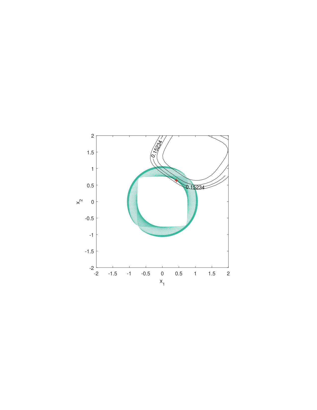 Figure 1
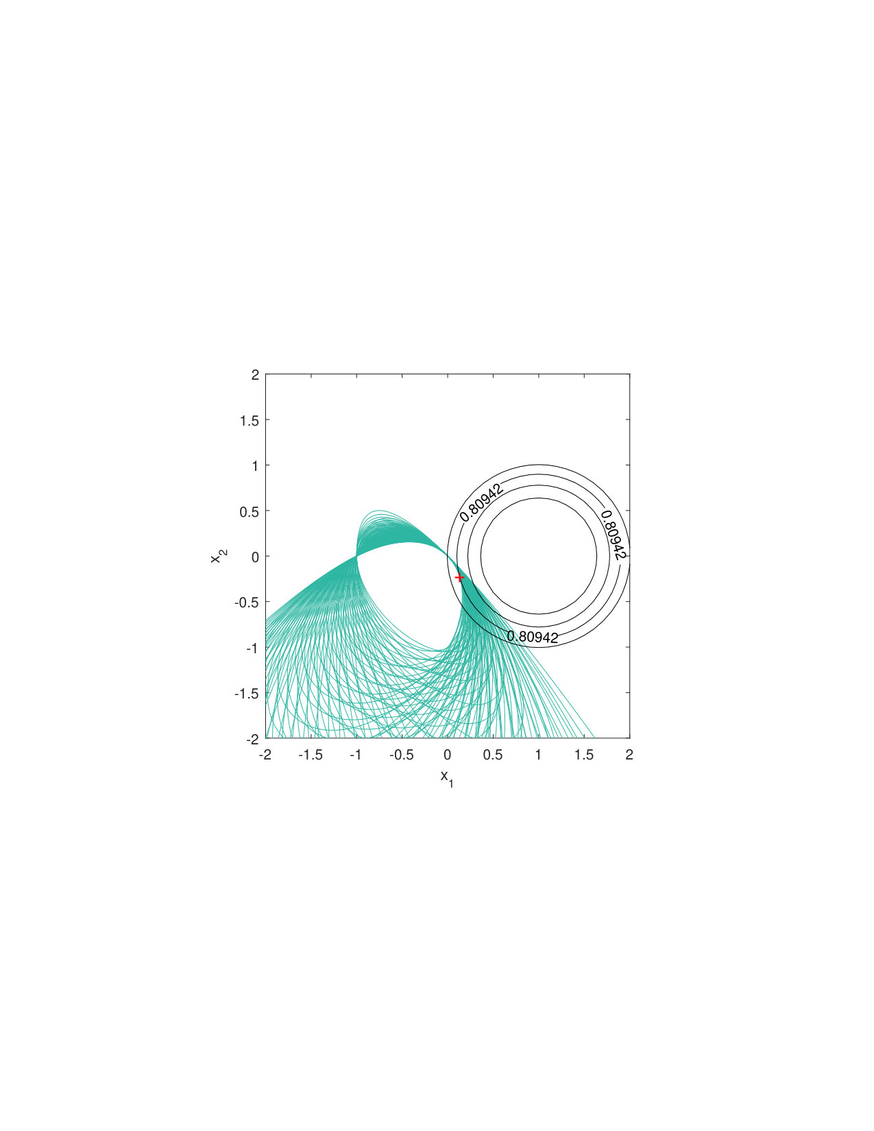 Figure 2
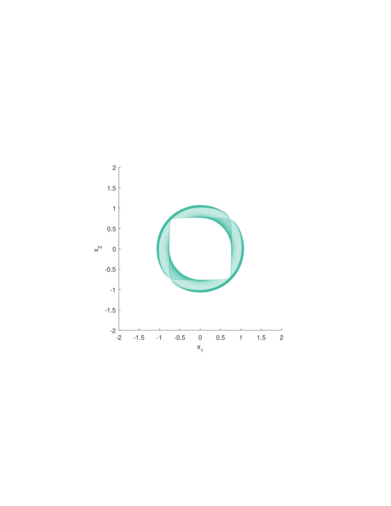 Figure 3
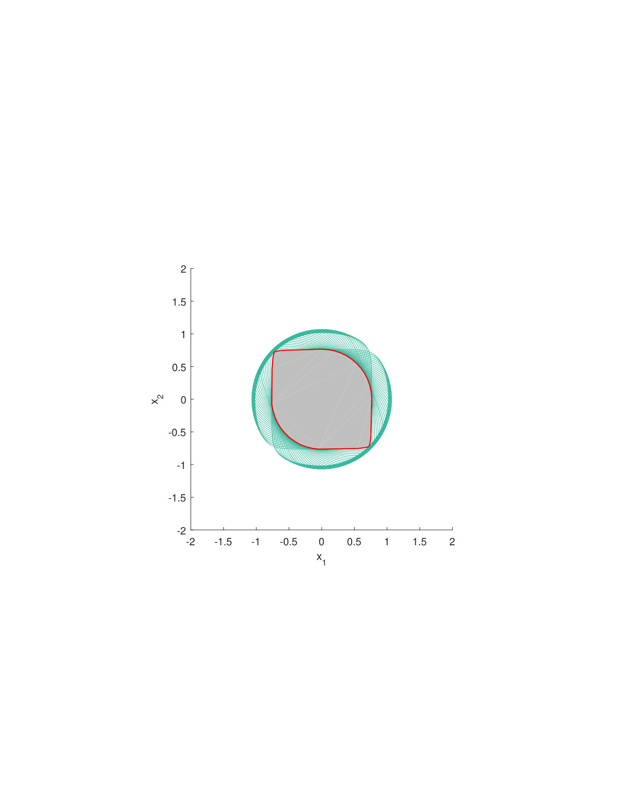 Figure 4
 Figure 5
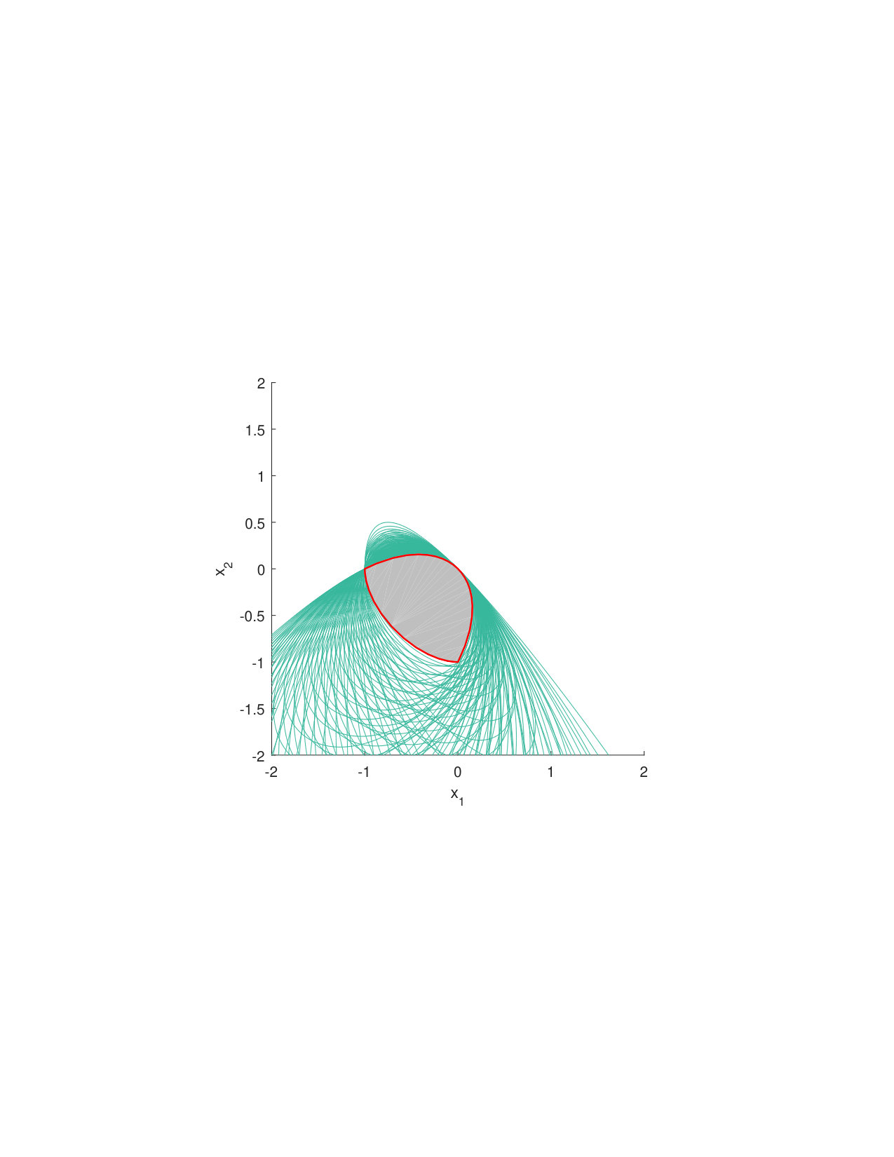 Figure 6
Peer Reviews
No public reviews on file for this paper yet. If you reviewed it on a platform where reviews are public (OpenReview, ICLR, NeurIPS, ICML), you can paste yours below so the community can read it here.
Videos
No videos yet. Explain this paper in a talk, walkthrough, or lecture? Add one.
Taxonomy
TopicsAdvanced Optimization Algorithms Research · Polynomial and algebraic computation · Advanced Control Systems Optimization
On semi-infinite systems of convex polynomial inequalities and
polynomial optimization problems
Feng Guo
School of Mathematical Sciences,
Dalian University of Technology, Dalian, 116024, China
Xiaoxia Sun
School of Mathematics,
Dongbei University of Finance and Economics, Dalian, 116025, China
Abstract
We consider the semi-infinite system of polynomial inequalities of the form
[TABLE]
where is a real polynomial in the variables and the parameters , the index set is a basic semialgebraic set in , is convex in for every . We propose a procedure to construct approximate semidefinite representations of . There are two indices to index these approximate semidefinite representations. As two indices increase, these semidefinite representation sets expand and contract, respectively, and can approximate as closely as possible under some assumptions. In some special cases, we can fix one of the two indices or both. Then, we consider the optimization problem of minimizing a convex polynomial over . We present an SDP relaxation method for this optimization problem by similar strategies used in constructing approximate semidefinite representations of . Under certain assumptions, some approximate minimizers of the optimization problem can also be obtained from the SDP relaxations. In some special cases, we show that the SDP relaxation for the optimization problem is exact and all minimizers can be extracted.
keywords:
semi-infinite systems, convex polynomials, semidefinite representations, semidefinite programming relaxations, sum of squares, polynomial optimization
MSC:
[2010] 65K05, 90C22, 90C34
1 Introduction
We consider the following semi-infinite system of polynomial inequalities
[TABLE]
where the polynomial ring in and over the real field and the index set is a basic semialgebraic set defined by
[TABLE]
where , . In this paper, we assume that is convex for every and hence is a convex set in .
We say a convex set in is semidefinitely representable (or linear matrices inequality representable) if there exist some integers and real symmetric matrices and such that is identical with
[TABLE]
and is called the semidefinite representation (or linear matrices inequality representation) of . Many interesting convex sets are semidefinitely representable, see a collection in Ben-Tal and Nemirovski (2001). Clearly, optimizing a linear function over a semidefinitely representable set can be cast as a semidefinite progamming (SDP) problem, while SDP has an extremely wide area of applications and can be efficiently solved by interior-point methods to a given accuracy in polynomial time (c.f. Wolkowicz et al. (2000)). Semidefinite representations of convex sets can help us to build SDP relaxations of many computationally intractable optimization problems. Arising from above, one of the basic issues in convex algebraic geometry is to characterize convex sets in which are semidefinitely representable and give systematic procedures to obtain their semidefinite representations. Clearly, if a set in is semidefinitely representable, then it is convex and semialgebraic. Conversely, Nemirovski asked in his plenary address at the 2006 ICM that whether each convex semialgebraic set is semidefinitely representable. Yet a negative answer has been recently given by Scheiderer (2018). Hence, it is reasonable to study how to construct approximate semidefinite representations of , that is a sequence of semidefinite representation sets of the form which converge to in some sence.
For a given basic semialgebraic set in , Lasserre (2009b) and Gouveia et al. (2010) proposed some methods to construct semidefinite outer approximations of the closure of its convex hull. These appproaches are based on the sums of squares representation of linear functions which are nonnegative on a basic semialgebraic set. If the basic semialgebraic set is compact, these approximations can be made arbitrarily close and become exact under some favorable conditions. Some extensions of these semidefinite approximations to noncompact basic semialgebraic sets are given in Guo et al. (2015). For a convex semialgebraic set, Helton and Nie (2009, 2010) proposed some sufficient conditions, in terms of curvature conditions for the boundary, for its semidefinite representability. These conditions are recently modified and improved by Kriel and Schweighofer (2018). In this paper, we first consider to construct approximate semidefinite representations of the set in (1). The difference of this problem from ones in the literature is that is defined by infinitely many convex real polynomials. As there is a quantifier in the definition (1), is in fact a semialgebraic set by the Tarski-Seidenberg principle (c.f. Bochnak et al. (1998)). Theoretically, can be decomposed as a finite union of basic closed semialgebraic sets and hence, as proved in Helton and Nie (2009), the semidefinite approximations of can be made by glueing together Lasserre (2009b) relaxations of many small pieces of . Such a decomposition of can possibly be obtained by quantifier elimination with algebraic techniques (c.f. Bochnak et al. (1998)). However, in practice (exact) quantifier elimination is very costly and limited to problems of very modest size. These obstacles make the problem studied in this paper nontrivial. To the best of our knowledge, there is very few related work in the literature addressing this issue. In Lasserre (2015); Magron et al. (2015), some tractable methods using semidefinite programs are proposed to approximate semi-algebraic sets defined with quantifiers. Clearly, the set studied in this paper is in such case with a universal quantifiers. However, rather than approximate semidefinite representations of , their approach generates a sequence of sublevel sets of a single polynomial to approximate .
In the second part of this paper, we consider the following convex minimization problem
[TABLE]
This problem is NP-hard. Indeed, it is obvious that the problem of minimizing a polynomial over can be regarded as a special case of . As is well known, the polynomial optimization problem is NP-hard even when , is a nonconvex quadratic polynomial and ’s are linear (c.f. Pardalos and Vavasis (1991)). Hence, a general the problem cannot be expected to be solved in polynomial time unless P=NP.
The problem can be seen as a special branch of convex semi-infinite programming (SIP), in which the involved functions are not necessarily polynomials. Numerically, SIP problems can be solved by different approaches including, for instance, discretization methods, local reduction methods, exchange methods, simplex-like methods and so on. See Hettich and Kortanek (1993); López and Still (2007); Goberna and López (2017) and the references therein for details. One of main difficulties in numerical treatment of general SIP problems is that the feasibility test of is equivalent to globally solve the lower level subproblem of which is generally nonlinear and nonconvex. To the best of our knowledge, few of the numerical methods mentioned above are specially designed by exploiting features of polynomial optimization problems. Parpas and Rustem (2009) proposed a discretization-like method to solve minimax polynomial optimization problems, which can be reformulated as semi-infinite polynomial programming (SIPP) problems. Using polynomial approximation and an appropriate hierarchy of SDP relaxations, Lasserre presented an algorithm to solve the generalized SIPP problems in Lasserre (2012). Based on an exchange scheme, an SDP relaxation method for solving SIPP problems was proposed in Wang and Guo (2013). By using representations of nonnegative polynomials in the univariate case, an SDP method was given in Xu et al. (2015) for linear SIPP problems (a special case of ) with being closed intervals.
Here are some contributions and novelties in this paper:
- (i)
We first propose a procedure to construct approximate semidefinite representations of (Section 3.2). The construction is based on some representations of linear functions nonnegative on . On the one hand, we use high degree perturbation proposed in Lasserre and Netzer (2007) to approximate the Lagrangian associated with the considered linear function by sums of squares of polynomials. As there is an integration with respect to some unknown measure in the Lagrangian, on the other hand, we employ Putinar’s Positivstellensatz to replace the integration by some linear functionals in the dual spaces of quadratic modules. Consequently, some semidefinite representation sets with two indices are obtained to approximate . As two indices increase, these semidefinite representation sets expand and contract, respectively, and can approximate as closely as possible under some assumptions (Theorem 3.7). In some special cases when we can fix one of the two indices or both (Remark 3.8). 2. (ii)
As the second contribution in this paper, we present some new SDP relaxation methods for the problem by similar strategies used in constructing approximate semidefinite representations of . Approximate values of can be obtaind by the proposed SDP relaxations with two indices and converge to as the two indices tend to (Theorem 4.4). If has a unique minimizer, approximate minimizers of can also be obtained from the SDP relaxations (Remark 4.5). Compared with some existing related work, the convexity in is well exploited here and the assumptions needed are quite mild. In the case when and are s.o.s-convex for every , the indices in the SDP relaxations can be reduced to one. If, moreover, is a bounded interval, we show that the SDP relaxation of is exact and all minimizers can be extracted (Theorem 4.8).
This paper is organized as follows. In Section 2, we give some notation and preliminaries used in this paper. Approximate semidefinite representations of as well as some examples are proposed in Section 3. We study SDP relaxations of the problem in Section 4.
2 Notation and Preliminaries
Here is some notation used in this paper. The symbol (resp., ) denotes the set of nonnegative integers (resp., real numbers). For any , (resp. ) denotes the smallest (resp. largest) integer that is not smaller (resp. larger) than . For , denotes the standard Euclidean norm of . For , . For , denote and its cardinality. For variables , and , , denote , , respectively. (resp., ) denotes the ring of polynomials in (resp., ) with real coefficients. For , denote by (resp., ) the set of polynomials in (resp., ) of total degree up to . For , denote by the dual space of linear functionals from to .
Definition 2.1
We say that the Slater condition holds for if there exists such that for all and the point is called a Slater point.
Theorem 2.2
(c.f. Borwein (1981); Levin (1969))* Assume that the Slater condition holds for and the index set is compact in the problem . Then for any convex , there exist points with such that is equal to the optimal value of the discretization problem*
[TABLE]
Corollary 2.3
Suppose that the assumptions in Theorem 2.2 hold for . Then for any convex , there exist , and nonnegative Lagrange multipliers with such that the Lagrangian
[TABLE]
satisfies that for all and .
Proof. Consider the discretization problem (4). As the Slater condition holds for (4), by convex programming duality (c.f. (Bertsekas, 2009, Proposition 5.3.1)), there is no dual gap between (4) with its Lagrange dual problem, which has an optimal solution, say where . By a Frank-Wolfe type theorem proved in Belousov (1977), (4) also has an optimal solution, say . Then, due to convex programming optimality conditions (c.f. (Bertsekas, 2009, Proposition 5.3.2)), we get
[TABLE]
which implies that for all and hence .
Next we recall some background about representations of polynomials positive (nonnegative) on a basic semialgebraic set and the dual theory. A polynomial is said to be a sum of squares (s.o.s) of polynomials if it can be written as for some . Notice that not every nonnegative polynomials can be written as s.o.s, see Reznick (2000). Lasserre and Netzer (2007) gave the following s.o.s approximations of nonnegative polynomials via simple high degree perturbations.
Theorem 2.4
(Lasserre and Netzer, 2007, c.f. Theorem 3.1, 3.2 and Corollary 3.3)* For a given , the following are true.*
- (i)
For any , there exists such that is s.o.s if and only if ; 2. (ii)
If is nonnegative on , then in decreasingly converges to [math] as tends to ; 3. (iii)
For any , if is nonnegative on , then there exists some such that is s.o.s for every .
Moreover, in Theorem 2.4 is computable by solving an SDP problem, see (Lasserre and Netzer, 2007, Theorem 3.1).
In the rest of this paper, we let be the set of polynomials that defines the semialgebraic set in and for convenience.
We denote by
[TABLE]
the quadratic module generated by and denote by
[TABLE]
its -th quadratic module. It is clear that if , then for any . However, the converse is not necessarily true. Note that checking for a fixed is an SDP feasibility problem, see Lasserre (2001); Parrilo and Sturmfels (2003).
Definition 2.5
We say that is Archimedean if there exists such that the inequality defines a compact set in .
Note that the Archimedean property implies that is compact but the converse is not necessarily true. However, for any compact set we can always force the associated quadratic module to be Archimedean by adding a redundant constraint in the description of for sufficiently large .
Theorem 2.6
(Putinar, 1993, Putinar’s Positivstellensatz)* Suppose that is Archimedean. If a polynomial is positive on , then for some . *
For a polynomial , define the norm
[TABLE]
We have the following result for an estimation of the order in Theorem 2.6.
Theorem 2.7
(Nie and Schweighofer, 2007, Theorem 6)* Suppose that is Archimedean and for some . Then there is some positive (depending only on ’s) such that for all of degree with , we have whenever*
[TABLE]
We say that a linear functional has a representing measure if there exists a Borel measure on such that
[TABLE]
For , we say has a representing measure if the above holds for all .
A basic problem in the theory of moments concerns the characterization of linear functionals in which have some representing measure.
Theorem 2.8
(Berg and Maserick, 1984, Theorem 2.1)* Let be a linear functional in such that for all . If there exist such that for every , then has exactly one representing measure on with support contained in .*
Haviland (1935) proved that has a representing measure supported on in (2) if and only if for every nonnegative on . Clearly,
[TABLE]
Hence, in a dual view, Putinar’s Positivstellensatz reads
Theorem 2.9
(Putinar, 1993, Putinar’s Positivstellensatz)* Suppose that is Archimedean. If for all , then has a representing measure supported on . *
Let
[TABLE]
For , we have the following sufficient condition for a linear functional having representing measure supported on . Denote by the -th moment matrix associated with a linear functional , which is indexed by , with -th entry for .
Condition 2.10
A linear functional satisfies the flat extension condition when
[TABLE]
Theorem 2.11
(Curto and Fialkow, 2005, Theorem 1.1)* Suppose that satisfies the flat extension condition with , then has a unique -atomic representing measure supported on . *
To end this section, let us recall a very interesting subclass of convex polynomials in introduced by Helton and Nie (2010).
Definition 2.12
(Helton and Nie (2010))* A polynomial is s.o.s-convex if its Hessian is a s.o.s, i.e., there is some integer and some matrix polynomial such that .*
While checking the convexity of a polynomial is generally NP-hard (c.f. Ahmadi et al. (2013)), s.o.s-convexity can be checked numerically by solving an SDP, see Helton and Nie (2010). The following result plays a significant role in this paper.
Lemma 2.13
(Helton and Nie, 2010, Lemma 8)* Let be s.o.s-convex. If and for some , then is s.o.s.*
3 Approximate semidefinite representations of
As we always assume that the index set in the definition of is compact in this paper, we first show that a set with a generic noncompact index set can be converted into a system with compact index set. Hereafter, by saying that a property holds for a generic index set , we mean that it holds for in the following sense. If we consider the space of all coefficients of generators ’s of all possible sets of form in the canonical monomial basis of with , then coefficients of ’s of those index sets such that the property does not hold are in a Zariski closed set of the space.
3.1 Noncompact case
In this subsection, we consider the set in (1) with noncompact index set . We used the technique of homogenization proposed in Wang and Guo (2013) to convert a semi-infinite system (1) with a generic noncompact index set into a system with compact index set.
For a polynomial , denote its homogenization by , where , i.e., . For the basic semialgebraic set in , define
[TABLE]
Proposition 3.1
(Wang and Guo, 2013, Proposition 4.2)* For any , on if and only if on .*
Let and be the homogenization of with respect to the variables . It follows that the set in is equivalent to
[TABLE]
Replacing by the basic semialgebraic set , we get the following set
[TABLE]
It is obvious that since .
Definition 3.2
(Nie (2013))* is said to be closed at if .*
Remark 3.3
Clearly, when is closed at . Note that not every set of form is closed at even when it is compact (Nie, 2012, Example 5.2). However, it is shown in (Wang and Guo, 2013, Theorem 4.10) that the closedness at is a generic property. It follows that for generic index sets . Note that depends only on , while depends not only on but also on the choice of the inequalities . In some cases, we can add some redundant inequalities in the description of to force it to be closed at (c.f. Guo et al. (2015)).**
For any polynomial , denote as its homogeneous part of the highest degree. Define
[TABLE]
In particular, denote as the homogeneous parts of with respect to of the highest degree .
Definition 3.4
We say that the extended Slater condition holds for if there exists a point of such that for all and for all . We call an extended Slater point of .
Proposition 3.5
The Slater condition holds for if and only if the extended Slater condition holds for .
Proof. Suppose that is an extended Slater point of . For any , we have if and otherwise. It is straightforward to verify that the Slater condition also holds for at .
Suppose that the Slater condition holds for at . For any point , we have if and if . Then similarly, it implies that the extended Slater condition holds for at . As a result of the above arguments, it is reasonable to consider the following assumption in the rest of this paper.
Assumption 3.6
The set is compact, is convex for any and the Slater condition holds for .
3.2 Approximate semidefinite representations of
We assume that in (1) is compact and a scalar such that for any is known. For , define
[TABLE]
It is clear that for any and . Denote by the unit ball in . Recall the notation in (7) and let
[TABLE]
For (resp., ), denote by (resp., ) the image of (resp., ) on regarded as an element in (resp., ) with coefficients in (resp., ), i.e., (resp., ). Hence, some notation, like , should cause no confusion once the dual spaces where the linear fuctionals and come from are specified in the context.
Theorem 3.7
Suppose that is compact. For any integers and , define
[TABLE]
Then, for any and for any . If Assumption 3.6 holds, then the following are true.
- (i)
For any , there exists an integer such that for every and , it holds that . If is Archimedean, then there exists integer such that for every and , it holds that . Consequently, converges to as and both tend to ; 2. (ii)
If the Lagrangian as defined in is s.o.s for every linear , then for any , . For any , if moreover, is Archimedean, then there exists integer such that for any , . Consequently, converges to as tends to for any .
Proof. For a fixed , there exists satisfying conditions in (10) for . Let be the restriction of on . Then, it is clear that satisfies all conditions in (10) for and thus . Similarly, if , then for any .
(i). Fix an and a point . Now we prove that there is some integer that does not depend on such that for every and , which implies that . By (Lasserre, 2009b, Lemma 5), there exist and statisfying and such that for any and . Consider the optimization problem . By Corollary 2.3, the associated Lagrangian as defined in (5) is nonnegative on for some and nonnegative . In particular, is nonnegative on . By Theorem 2.4 (iii), there is some integer such that for any , it holds that
[TABLE]
for some . As , we have . Now we show that does not depend on . According to (Lasserre and Netzer, 2007, Sec. 3.3), depends on , the dimension and the size of , , ’s and the coefficients regarded as polynomials in . Fix a Slater point , since , as proved in (Lasserre, 2009b, Lemma 7), we have
[TABLE]
where since is a Slater point and is compact. Write , then . Hence, all , , ’s and ’s are uniformly bounded, which means that does not depend on . For any and , to the contrary, assume that . Then, there exists satisfying the conditions in (10) for with . Let where denotes the Dirac measure at . As , it holds that
[TABLE]
which is a contradiction. Thus, and .
Fix a Slater point . Let be arbitrary. Now we first prove that there exist a point and an integer that does not depend on (in fact, it depends on ’s) such that and for every and , which implies that . If , then let ; otherwise, let and , then we have , and
[TABLE]
Let . Then, in either case, it follows that
[TABLE]
for any . Write . Recall the norm defined in (6), then
[TABLE]
As is compact, is well-defined. Note that does not depend on but only on and . By Theorem 2.7, there exists come positive depending on ’s such that whenever
[TABLE]
For any , define a linear functional by for all . Then, it is clear that for , for and for all . We have . It implies that and thus for every and .
(ii). By (i), we only need to prove for any and . Fix a point . By the Separation Theorem of convex sets, there exist and such that for any and . As proved in (i), there are some and nonnegative such that is nonnegative on . Since the associated Lagrangian is s.o.s for every linear function , we have
[TABLE]
for some . To the contrary, assume that . Then, there exist satisfying the conditions in (10) for . Define as in (i). Like in (12), we get that
[TABLE]
which is a contradiction. Thus, and hence .
Remark 3.8
(i). According to the proof, the conclusions (i) and (ii) in Theorem 3.7 are still true if we simplify the condtion in by .
(ii). In practice, we can let in and approximate by one sequence . Suppose that is Archimedean, then by Theorem 3.7 (i), for any , there exists such that and . That is, can approximate as closely as possible as increases.
(iii). If is compact but is not Archimedean, then the set in the definition of in can be replaced by the -th order preordering in Schmüdgen’s representations of polynomials positive on (Schmüdgen (1991)). Moreover, if we have exact representations of polynomials nonnegative on in some cases, we may fix the order in and only let increase. Then, a sequence of nested outer approximate semidefinite representations of can be obtained. For instance, consider the case
[TABLE]
By the representations of univariate polynomials nonnegative on an interval (c.f. Powers and Reznick (2000); Laurent (2009)), we can fix and then the sequence converges to as tends to . We leave the details here to keep the paper clean.
(iv). If the Lagrangian is s.o.s for every linear , by the proof of Theorem 3.7 (ii), the condition is redundant and can be removed. In general, it may be difficult to check whether or not the Lagrangian is s.o.s for every linear . However, when is s.o.s-convex in for any , by Corollary 2.3 and Lemma 2.13, is indeed s.o.s for any s.o.s-convex (in particular, for every linear ). In particular, if is in the case (15) and is s.o.s-convex in for any , then we have the exact semidefinite representation for any and . * *
Note that the standard semidefinite representation (3) of can be easily generated using Yalmip (Löfberg (2004)). Moreover, for and , we can first generate the form (3) of and then draw it using the software package Bermeja Rostalski (2010).
Example 3.9
Now we present some illustrating examples. As we shall see, the approximate semidefinite representations defined in this section are very tight for some given sets .
- (1).
Consider the polynomial
[TABLE]
It is proved in Ahmadi and Parrilo (2012) that is convex but not s.o.s-convex. Rotate the shape in the -plane defined by continuously around the origin by clockwise. Denote by the common area of these shapes in this process. We illustrate in the left of Figure 1. In other words, the set is defined by
[TABLE]
where and
[TABLE]
It is clear that the assumptions in Theorem 3.7 holds for and , . By the software Bermeja, the semidefinite representation set as defined in is drawn in gray bounded by the red curve in the right of Figure 1.
- (2).
Consider the set
[TABLE]
where and
[TABLE]
We illustrate in the left of Figure 2 by using some grid of . The Hessian matrix of with respect to and is
[TABLE]
Clearly, is s.o.s-convex in for every . We have and . The semidefinite representation set is drawn in gray bounded by the red curve in the right of Figure 2.
3.3 More discussions
Now we would like to interpret the semidefinite approximations for in a dual view. We shall explain why these semidefinite approximations need two indices and whether or not we can approximate the convex hull of in a similar way if the convexity in is removed from the constraints functions for .
It is clear that the convex hull of a subset in is the intersection of half spaces defined by hyperplanes tangent to this subset. Hence, to obtain semidefinite approximations of the convex hull of a subset in , it is key to characterize linear functions nonnegative on the subset via s.o.s of polynomials. If is defined by finitely many polynomial inequalities, a linear function nonnegative on can be represented by Putinar’s (or Schmüdgen’s) Positivstellensatz and convergent semidefinite approximations of can be derived by increasing the degrees of s.o.s of polynomials invloved in the representation, see Lasserre (2009b); Gouveia et al. (2010). However, as the set in our case is defined by infinitely many polynomial inqualities, the Positivstellensatz can not be directly used here. Nevertheless, when is convex in for all and the assumptions in Corollary 2.3 hold, there exists a (atomic) measure supported on for each such that the associated Lagrangian on . Then, to obtain semidefinite approximations of , we can use Lasserre’s s.o.s representation via high degree perturbations (Theorem 2.4) to characterize this inequality and the dual of Putinar’s Positivstellensatz (Theorem 2.9) to replace the unknown measure by a linear functional in . Consequently, in the dual, the resulting semdefinite approximations are defined in the way (10) and need two indices, i.e., one to bound the degree of the perturbation and the other to bound the order of the quadratic module.
From the above arguments, we can also see that if the convexity in is removed from for , the convex hull of can not be approximated as closely as possible in a way similarly as is defined. To see this, recall that even in the finitely many constraints case mentioned above, one need to increase the degree of s.o.s of polynomials involved in the Putinar’s (or Schmüdgen’s) representation of to obtain convergent semidefinite approximations. In the infinitely many constraints case, to formulate the nonnegative Lagrangian , we need a measure for to encode those active (Corollary 2.3). As is unknown, we can not further parameterize unknown s.o.s of polynomials in the integral and increase the degree; otherwise, bi-linearity occurs and thus semidefinite approximations can not be derived. Moreover, such a measure for may not even exist if the convexity in is removed from . Therefore, it is still a challenge to construct semidefinite approximations of convex hull of semi-algebraic sets defined by infinitely many arbitrary polynomial inequalities. In Lasserre (2015); Magron et al. (2015), some tractable methods using semidefinite programs are proposed to approximate semi-algebraic sets defined with quantifiers. Clearly, the set studied in this paper is in such case with a universal quantifiers. To end this section, we would like to point out the differences in methodology and contributions between the present paper and the above two references. The following is the basic idea of Lasserre (2015); Magron et al. (2015) to get approximations of in (1). For , define the map . Then, we have . Suppose that is contained in a compact set in , then it can be proved that there exsits a sequence of polynomials such that for all and converges to for the -norm. Hence, can be approximated by . As for every and , we can use Positivstellensatz in to reduce the problem of computing such a sequence to SDP problems. Therefore, the method in Lasserre (2015); Magron et al. (2015) works for in a general form without requiring to be convex in and approximates by a sequence of sublevel set of a single polynomial. Instead, we exploit the convexity of the defining polynomials of and construct semidefinite approximations for it. Note that the polynomials ’s in method of Lasserre (2015); Magron et al. (2015) can be enforced to be convex for in (1) (see (Lasserre, 2015, Section 4.2)), but the convergence and the semidefinitely representability of the sublevel sets are not clear to the best of our knowledge.
4 SDP relaxations of convex semi-infinite polynomial
programming
For a convex polynomial , consider the following convex semi-infinite polynomial programming problem
[TABLE]
Let and be the set of all (nonnegative) Borel measures supported on .
4.1 General case
Consider the case when is compact and Assumption 3.6 holds. In the following, we will obtain SDP relaxations of in two steps.
In the first step, for any integer , we convert to the problem
[TABLE]
For , , , , and , consider the Lagrange dual function of (16):
[TABLE]
Then,
[TABLE]
Hence, the Lagrange dual problem of (16) reads
[TABLE]
Definition 4.1
We call with a nearly optimal solution of if is feasible for and the limit of is equal to the limit of the optimal values of as .
Theorem 4.2
Suppose that is convex, is compact and Assumption 3.6 holds. Let be a nearly optimal solution of and .
- (i)
* and converges to as tends to ;* 2. (ii)
* is attainable in and there is no dual gap between and ;* 3. (iii)
Assume that possibly after scaling. Then, for any convergent subsequence of , is a minimizer of . Consequently, if is the unique minimizer of , then ; 4. (iv)
If moreover, the Lagrangian as defined in is s.o.s, then for any and it is also attainable in .
Proof. (i) For any and , we have and . Consequently, for any feasible point of (16) and any , it holds that
[TABLE]
which implies that .
Conversely, by Corollary 2.3, there exist some and nonnegative Lagrange multipliers such that
[TABLE]
where and is the Dirac measure at . For any fixed with , by Theorem 2.4 (i), there exists a such that
[TABLE]
if and only if . It means that is feasible and . Moreover, by Theorem 2.4 (ii), decreasingly converges to [math] as tends to . It then follows that converges to as tends to .
(ii) Fix a Slater point of . Since is compact, there exists a neighborhood of such that every point in is a Slater point of . Let be the probability measure with uniform distribution in and set where . It is easy to see that is strictly admissible for (17). The conclusion follows due to the duality theory in convex optimization.
(iii) For any , as and , it is clear that for all . Since and for all , we then deduce that for any by (Lasserre and Netzer, 2007, Lemma 4.1 and 4.3). Extend to by letting for all and denote it by . Then, it holds that for all .
Let be a convergent subsequence of . By Tychonoff’s theorem, there exists a convergent subsequence of the corresponding in the product topology. Without loss of generality, we assume that the whole sequence converges as and denote by the limit. From the pointwise convergence, we have for all and for all . By Theorem 2.8, has exactly one representing measure with support contained in . Since is nearly optimal solution of (17), we obtain by (i) and (ii). We have
[TABLE]
For any , from the proof of Theorem 3.7 (i) and Remark 3.8 (i), it is easy to see that there exists an integer such that whenever . By the pointwise convergence, we deduce that . Then, since is convex and has a representing measure, by Jensen’s inequality, . Hence, is indeed a minimizer of (17).
Assume that is the unique minimizer of (17). We have shown that is contained in and for any convergent subsequence , therefore the whole sequence converges to .
(iv) Under the assumption, (19) holds for and any . Hence, for any by the proof of (i). As is compact, suppose that is attainable in at a minimizer . Define by letting for all , then is attainable in (17) at .
Consider the problem . The integration can be seen as a linear functional in . In the second step, to obtain SDP relaxations of , we need to characterize those linear functionals which have representing measures in . In a dual view, we need a representation of in (17) which is nonnegative on . Here, Putinar Positivstellensatz (Theorem 2.6 and 2.9) comes into play.
For any , consider the SDP relaxation of (16)
[TABLE]
Similar to (16), the Lagrange dual function of (20) is
[TABLE]
where , , , , and . Similar to the duality between (16) and (17), the Lagrange dual problem of (20) can be derived as
[TABLE]
Theorem 4.3
For any integer , the following are true.
- (i)
If is Archimedean and the Slater condition holds for , then and decreasingly converge to as tends to ; 2. (ii)
For some order , if the flat extension condition holds for in the solution of , then ; 3. (iii)
If is in the case (15), then we have .
Proof. (i) For any feasible point of (16), define by letting for all , then is feasible for (20) and hence for any . Then by the weak duality and Theorem 4.2, we have for any . It is sufficient to prove that .
Fixing an arbitrary , we show that there is some such that . Fix a Slater point of and define with for all . Then is feasible for (21) for some by Putinar’s Positivstellensatz. If , then . Next, we assume that . Then, we can choose another feasible point of (17) such that and . Let
[TABLE]
Then, we have and hence
[TABLE]
Hence, is feasible for (21) for some by Putinar’s Positivstellensatz. We have
[TABLE]
As is arbitrary, the conclusion follows.
(ii) Suppose that the flat extension condition holds for in the solution of (20) at some order . Then, by Theorem 2.11, admits some representing measure supported on . As and is feasible for (16), we conclude that .
(iii) By the proof of (i), the conclusion follows due to the representations of univariate polynomials nonnegative on an interval (c.f. Powers and Reznick (2000); Laurent (2009)) and Theorem 4.2 (ii).
Theorem 4.4
Suppose is convex , is compact and Assumption 3.6 holds. Then, for any , the following are true.
- (i)
There exists a such that holds for any and ; 2. (ii)
If is Archimedean and the Slater condition holds for , then for any , there exists a such that holds for any ; 3. (iii)
If is in the case (15), we have .
Proof. (i) It is clear that holds for any and . By Theorem 4.2 (i), there exists a such that holds for any . Thus, (i) follows.
(ii) Due to Theorem 4.3 (i), for any , there exists a such that holds for any . Then (ii) follows since for any by Theorem 4.2 (i).
(iii) It is clear by Theorem 4.2 (i) and Theorem 4.3 (iii).
Remark 4.5
(i). Theorem 4.4 (i) and (ii) implies that we can approximate by and as closely as possible with and both large enough. In practice, we can let and then under the assumptions in Theorem 4.4 (i) and (ii).
(ii). Assume that . By Theorem 4.3 i, for any , there exists such that . Denote by a minimizer of , then is a sequence of nearly optimal solutions of and Theorem 4.2 (iii) holds for the corresponding sequence . In particular, when has a unique minizer and are large enough, we can expect that the point for any approximate solution of lies in a small neighborhood of . * *
4.2 S.O.S-Convex case
Recall Remark 3.8 (iv) and Theorem 4.2 (iv). We now strengthen Assumption 3.6 to
Assumption 4.6
The set is compact, is s.o.s-convex for any and the Slater condition holds for .
If Assumption 4.6 holds and is s.o.s-convex, then the Lagrangian as defined in (5) is s.o.s according to Remark 3.8 (iv). Like in the general case, in the first step, we convert to
[TABLE]
For , , and , consider the Lagrange dual function of (22):
[TABLE]
Then,
[TABLE]
Hence, the Lagrange dual problem of (16) reads
[TABLE]
Theorem 4.7
*Assume that is s.o.s-convex and Assumption 4.6 holds, then the following are true. *
- (i)
The optimal values of and are both equal to which is attainable in . Moreover, if is attainable in , then so it is in ; 2. (ii)
If is a minimizer of , then is a minimizer of .
Proof. (i) Denote by the optimal value of (22). Since Assumption 3.6 holds, recalling (18), there exists such that for all . Note that the degree of is even and at most . As is s.o.s, it holds that
[TABLE]
which means that (22) is feasible and . For any and feasible point of (22), it holds that which implies that . Consequently, we have . Since (23) is strictly feasible (see the proof of Theorem 4.2 (ii)), (22) has an optimal solution and there is no dual gap between (22) and (23).
Suppose that is attainable in at a minimizer . Define by letting for all , then is attainable in (23) at .
(ii) Compare the feasible set of (23) with the definition of in (10) and recall the proof of Theorem 3.7 (ii). Note that to show for any and , the constraints in (10) are redundant. Moreover, the inequality (14) still holds for feasible to (23). Hence, we can obtain that . As is s.o.s-convex, by (Lasserre, 2009a, Theorem 2.6), the extension of Jensen’s inequality holds, which implies that is a minimizer of .
In the same way as we derive the SDP relaxations (20) and (21) from (16) and (17), we next obtain corresponding SDP relaxations of (22) and (23) as
[TABLE]
and its dual
[TABLE]
Theorem 4.8
*Assume that is s.o.s-convex and Assumption 4.6 holds, then the following are true. *
- (i)
If is Archimedean and the Slater condition holds for , then ; 2. (ii)
For some order , if the flat extension condition holds for in the solution of , then ; 3. (iii)
Let be a sequence of nearly optimal solutions of and . For any convergent subsequence of , is a minimizer of . Consequently, if is bounded and is a unique minimizer of , then . 4. (iv)
If is in the case (15), then we have . If is solvable, then is a minimizer of if and only if there exists a minimizer of with such that .
Proof. (i) and (ii): See Theorem 4.7 (i) and the proofs of Theorem 4.3 (i) and (ii).
(iii): Since is s.o.s-convex, due to the extended Jensen’s inequality (Lasserre, 2009a, Theorem 2.6), it holds that and therefore . From the proofs of Theorem 3.7 (ii) and Theorem 4.7 (ii), it is easy to see that the sequence and hence . Thus, is a minimizer of .
(iv): By Theorem 4.7 (i) and the weak duality, it holds that for any . For any , there exists a point such that . Define by letting for all . By the representations of univariate polynomials nonnegative on an interval (c.f. Powers and Reznick (2000); Laurent (2009)), is feasible to (25) with , which implies that . Since is abitrary, it holds that .
Clearly, we only need to prove the “if” part. Since Assumption 4.6 holds, from the proofs of Theorem 3.7 (ii) and Theorem 4.7 (ii), we have . As is s.o.s-convex, due to the extended Jensen’s inequality (Lasserre, 2009a, Theorem 2.6), it holds that . Thus, is a minimizer of .
Remark 4.9
(i) Note that we do not require to be compact in Theorem 4.7 and 4.8.
(ii) In the special case when are linear in for every , the SDP relaxation (24) agrees with the SDP relaxation of generalized problems of moments proposed in Lasserre (2008). * *
Example 4.10
Now we consider two convex semi-infinite polynomial programming problems using the sets defined in Example 3.9 (1) and (2). Notice that the constraints in the dual SDP relaxations and can be easily generated by Yalmip. Hence, we solve the following problems using these corresponding dual SDP relaxations, which can also give us some informations on the minimizers of the problems.
- (1).
Recall the sets and defined in Example 3.9 (1) where the polynomial is convex but not s.o.s-convex for every . Ahmadi and Parrilo (2013)* constructed a polynomial*
[TABLE]
see (Ahmadi and Parrilo, 2013, (5.2)) which is convex but not s.o.s-convex. In order to illustrate the efficiency of the SDP relaxations better, we shift and scale to define , which is still convex but not s.o.s-convex. Then, consider the problem , where . Letting , we get achieved at and an approximate minimizer . To show the accuracy of the solution, we draw some contoure lines of , including , and mark the point by red ‘’ in Figure 3 (left). As we can see, the line is almost tangent to at the point . 2. (2).
Recall the sets and defined in Example 3.9 (2). Let , i.e., the square of the distance function of a point to , and consider the problem . Then, the polynomials and for all are s.o.s-convex. As , solving the SDP relaxation with , we get achieved at and an approximate minimizer . The corresponding contoures and the point are shown in Figure 3 (right).
To end this section, we compare our SDP relaxation method for the convex semi-infinite polynomial programming problem with the approach given in Wang and Guo (2013), which can also solve via SDP relaxations. In fact, the method proposed in Wang and Guo (2013) is based on the exchange scheme and works for semi-infinite polynomial programming problems without requiring convexity.
Generally speaking, given a finite subset in an iteration, one obtains at least one global minimizer of under the associated finitely many constraints and then compute the global minimum and minimizers of over . If , stop; otherwise, update and proceed to the next iteration. Therefore, to guarantee the success of the exchange method, the subproblems in each iteration need to be globally solved and at least one minimizer of each subproblem can be extracted. The subproblems can be solved by Lasserre’s SDP relaxation method and minimizers can be extracted when the flat extension condition holds.
However, Lasserre’s SDP relaxation method for the lower level subproblem of minimizing over does not necessarily have finite convergence. Even it does, a minimizer for the lower level subproblem could not be extracted. In particular, when there are infinitely many minimizers, the flat extension condition fails (c.f. (Laurent, 2009, Sec. 6.6)). For polynomial optimization problems with generic coefficients data, according to (Nie, 2014, Theorem 1.2) and (Nie and Ranestad, 2009, Proposition 2.1), there are finitely many minimizers and Lasserre’s SDP relaxation method has finite convergence. However, even the coefficients data in is generic, we are not clear about the success of the method in Wang and Guo (2013) applied to . It is because in the lower level subproblems, the coefficients of depend on the solutions of the upper level subproblem of the same interation.
For example, consider the problem
[TABLE]
It is easy to see that the feasible set is and the minimizer is . If we choose the intial set , then upper level subproblem has a unique minimizer . Then for the lower level subproblem of minimizing over , it clear that the solution set is which is infinite and the flat extension condition does not apply for Lasserre’s SDP relaxations. As none of the minimizers can be extracted, the method in Wang and Guo (2013) fails for this problem. Since the objective functions is s.o.s-convex and Assumption 4.6 holds, we can solve the above problem by our SDP relaxations . Let , we get achieved at and an approximate minimizer .
Acknowledgments
The authors are very grateful for the comments of two anonymous referees which helped to improve the presentation. The first author was supported by the Chinese National Natural Science Foundation under grants 11401074, 11571350. The second author was supported by the Chinese National Natural Science Foundation under grant 11801064, the Foundation of Liaoning Education Committee under grant LN2017QN043.
The reference list from the paper itself. Each links out to its DOI / PubMed record.
- 1Ahmadi and Parrilo (2013) Ahmadi, A., Parrilo, P., 2013. A complete characterization of the gap between convexity and sos-convexity. SIAM Journal on Optimization 23 (2), 811–833.
- 2Ahmadi et al. (2013) Ahmadi, A. A., Olshevsky, A., Parrilo, P. A., Tsitsiklis, J. N., 2013. NP-hardness of deciding convexity of quartic polynomials and related problems. Mathematical Programming 137 (1), 453–476.
- 3Ahmadi and Parrilo (2012) Ahmadi, A. A., Parrilo, P. A., Oct 2012. A convex polynomial that is not sos-convex. Mathematical Programming 135 (1), 275–292.
- 4Belousov (1977) Belousov, E., 1977. Introduction to Convex Analysis and Integer Programming. Moscow University Publ.: Moscow.
- 5Ben-Tal and Nemirovski (2001) Ben-Tal, A., Nemirovski, A., 2001. Lectures on Modern Convex Optimization: Analysis, Algorithms, and Engineering Applications. MOS-SIAM Series on Optimization. Society for Industrial and Applied Mathematics.
- 6Berg and Maserick (1984) Berg, C., Maserick, P. H., 1984. Exponentially bounded positive definite functions. Illinois Journal of Mathematics 28, 162–179.
- 7Bertsekas (2009) Bertsekas, D. P., 2009. Convex optimization theory. Athena Scientific.
- 8Bochnak et al. (1998) Bochnak, J., Coste, M., Roy, M.-F., 1998. Real Algebraic Geometry. Springer.