Global dynamics of the real secant method
Antonio Garijo, Xavier Jarque

TL;DR
This paper analyzes the secant method for root finding as a dynamical system, exploring basin structures, stability, and extending the method to a topological space to improve understanding and efficiency.
Contribution
It provides a detailed dynamical systems perspective on the secant method, including basin analysis and an extension to the punctured torus for better root-finding insights.
Findings
Basin shapes and distributions for roots are characterized.
Existence of stable dynamics affecting algorithm efficiency is shown.
Extension to the punctured torus enhances understanding of behavior near infinity.
Abstract
We investigate the root finding algorithm given by the secant method applied to a real polynomial as a discrete dynamical system defined on . We study the shape and distribution of the basins of attraction associated to the roots of , and we also show the existence of other stable dynamics that might affect the efficiency of the algorithm. Finally we extend the secant map to the punctured torus which allow us to better understand the dynamics of the secant method near and facilitate the use of the secant map as a method to find all roots of a polynomial.
Click any figure to enlarge with its caption.
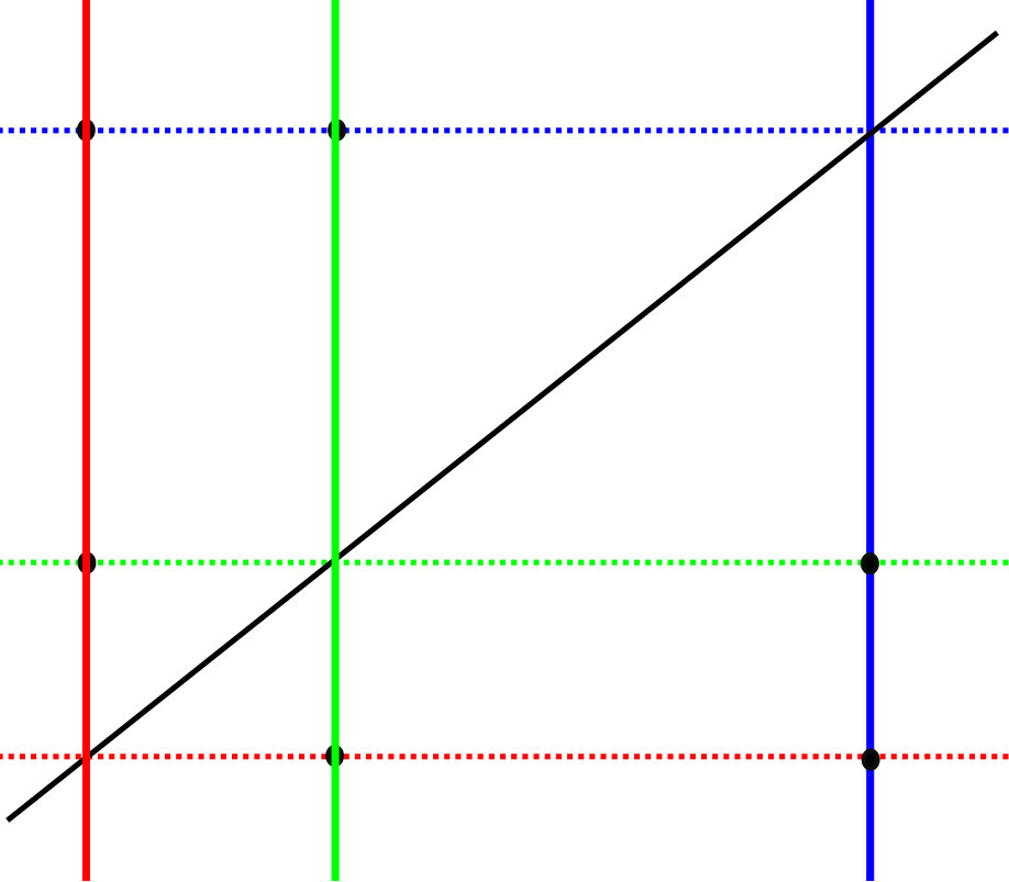 Figure 1
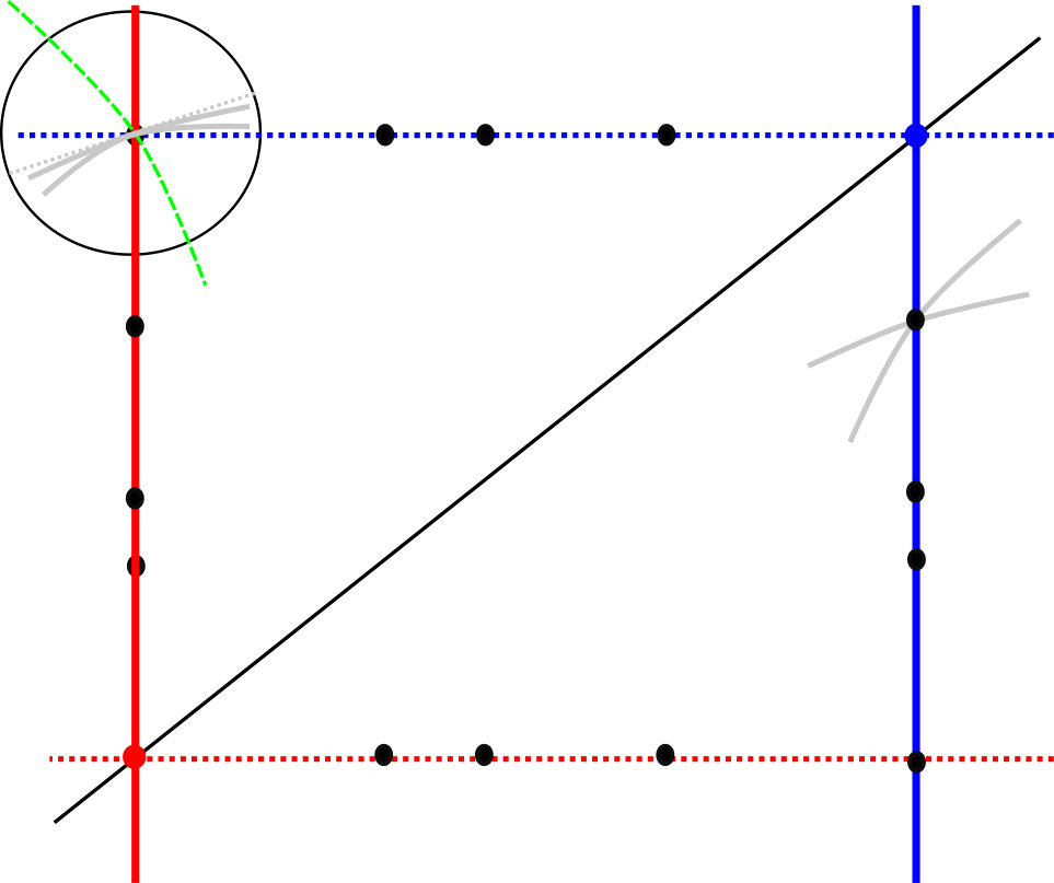 Figure 2
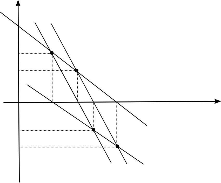 Figure 3
 Figure 4
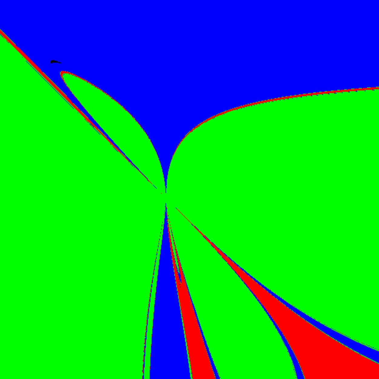 Figure 5
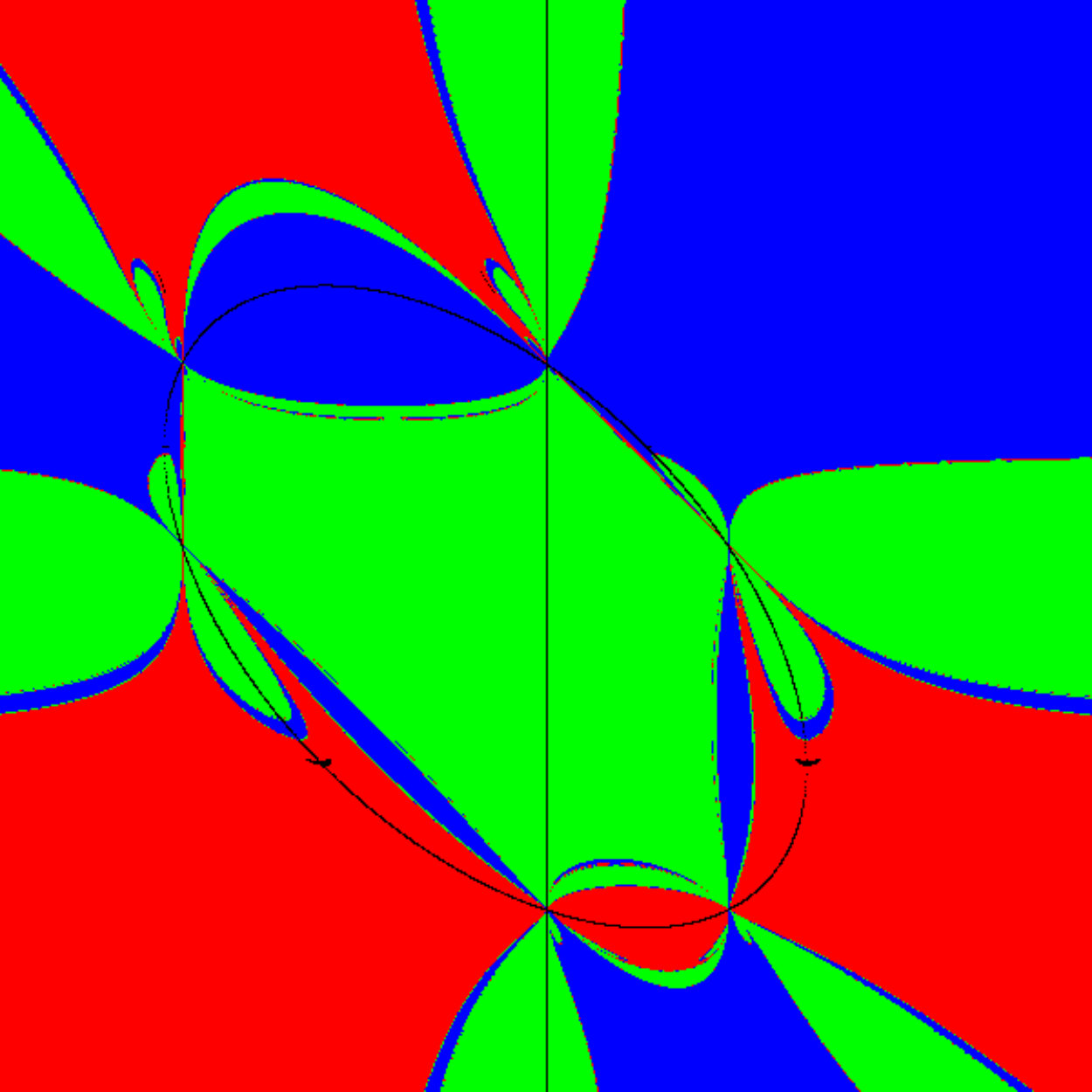 Figure 6
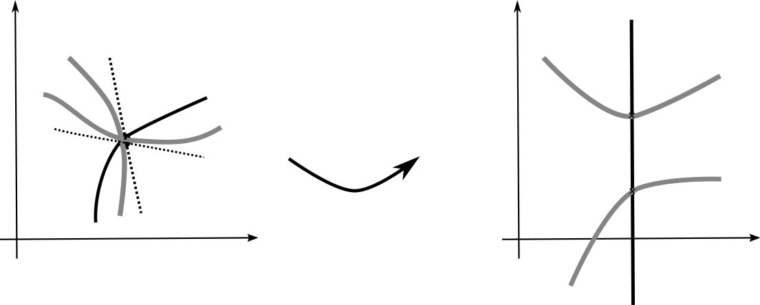 Figure 7
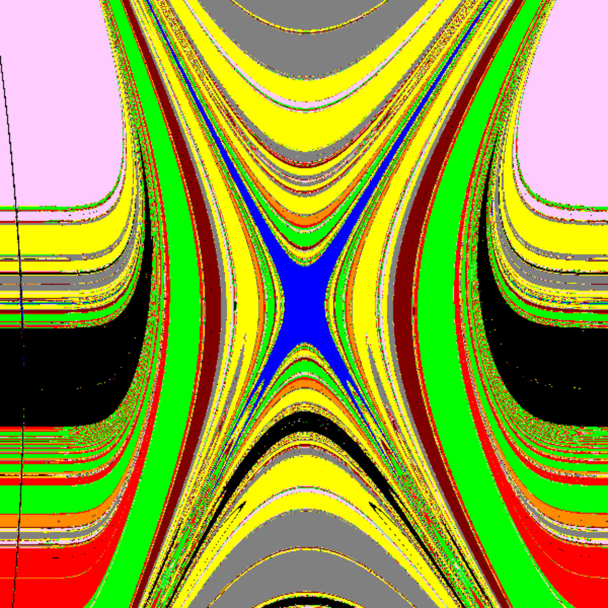 Figure 8
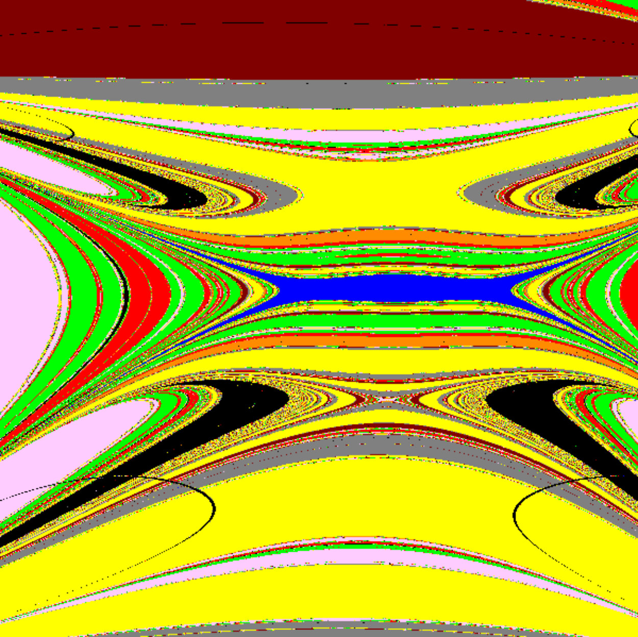 Figure 9
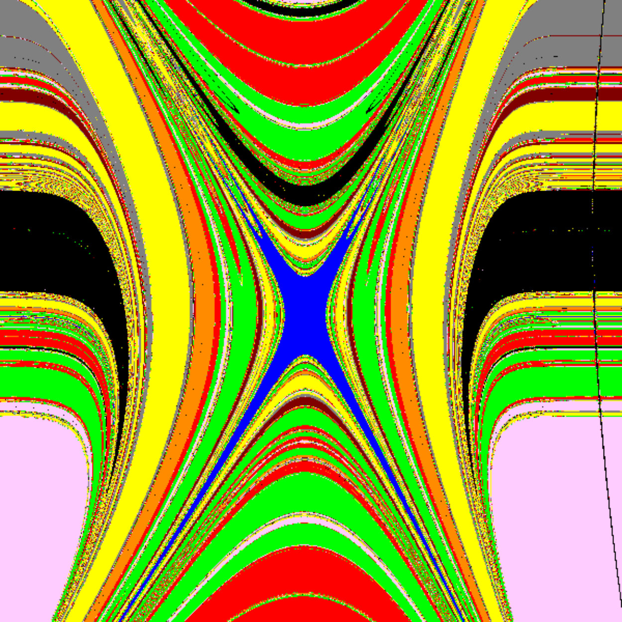 Figure 10
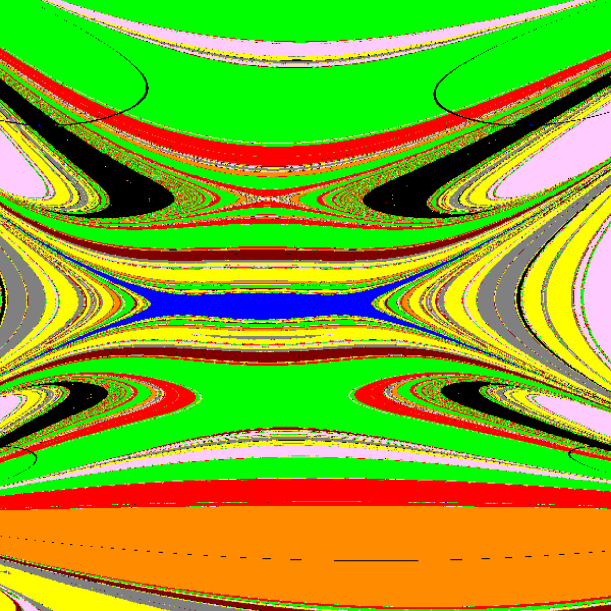 Figure 11
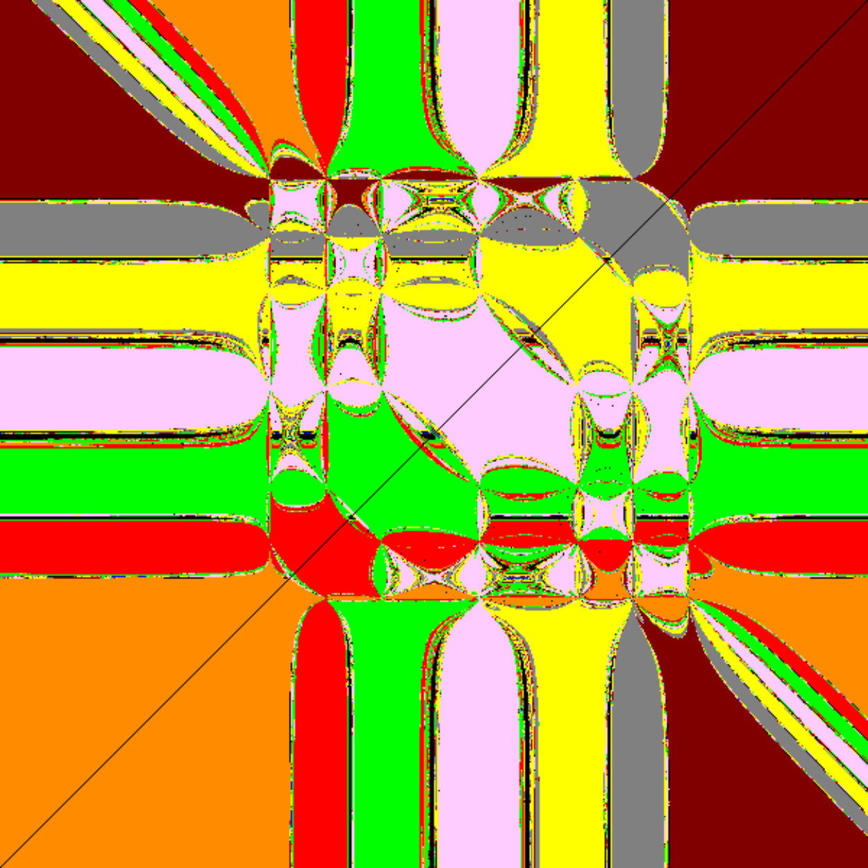 Figure 12
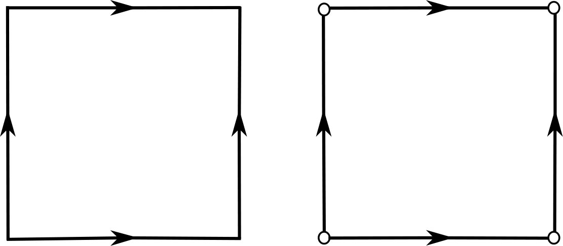 Figure 13
Peer Reviews
No public reviews on file for this paper yet. If you reviewed it on a platform where reviews are public (OpenReview, ICLR, NeurIPS, ICML), you can paste yours below so the community can read it here.
Videos
No videos yet. Explain this paper in a talk, walkthrough, or lecture? Add one.
Global dynamics of the real secant method
Antonio Garijo
Departament d’Enginyeria Informàtica i Matemàtiques, Universitat Rovira i Virgili, 43007 Tarragona, Catalonia.
and
Xavier Jarque
Departament de Matemàtiques i Informàtica at Universitat de Barelona and Barcelona Graduate School of Mathematics, 08007 Barcelona, Catalonia.
Abstract.
We investigate the root finding algorithm given by the secant method applied to a real polynomial as a discrete dynamical system defined on . We study the shape and distribution of the basins of attraction associated to the roots of , and we also show the existence of other stable dynamics that might affect the efficiency of the algorithm. Finally we extend the secant map to the punctured torus which allow us to better understand the dynamics of the secant method near and facilitate the use of the secant map as a method to find all roots of a polynomial.
Keywords: Root finding algorithms, dynamical systems, secant method
This work has been partially supported by MINECO-AEI grants MTM-2017-86795-C3-2-P and MTM-2017-86795-C3-3-P, and the AGAUR grant 2017 SGR 1374
1. Introduction
Root finding algorithms
[TABLE]
are iterative systems so that for most initial seeds the sequence converges to a solution of a given nonlinear equation, namely . Since many real problems can be modelled in terms of nonlinear equations which do not admit explicit solutions, the applicability of those algorithms is wide over all areas like engineering, economics, sociology or biology. Through the whole paper we will assume that is a polynomial of degree at least 2 and hence our goal is to solve the equation with .
There are many natural questions about the efficiency of those algorithms. If the equation has more than one solution, as it happens in most cases, how to find different seeds converging to each of them? Is it possible to have regions with positive measure where seeds do not converge to any solution of ? What can be said about the speed (number of steps) to have a reasonable approximation of the solution (order of convergence)? To answer these questions, or more ambitious, to have a deeper understanding of those algorithms, we treat them as discrete dynamical systems (see, for instance, [HSS01]).
Roughly speaking a discrete dynamical system over is a map and the orbits induced by this map starting at , that is, where
[TABLE]
A main goal when studying dynamical systems is to describe the asymptotic behaviour of those orbits when runs over all . In particular the study of fixed points, i.e. in such that . Those points are classified according to the behaviour of the nearby seeds and play a key role on the global dynamics. In particular, a fixed point in is called attracting if there exists such that , as , for all in . Accordingly, given an attracting fixed point , its basin of attraction is denoted by and given by
[TABLE]
which it is open and nonempty by definition. The connected component of which contains is called the immediate basin of attraction of and it is denoted by . We also consider periodic points of (minimal) period , or -periodic points, i.e. in such that there exist satisfying and for all . Similarly, we can define attracting -periodic points and their attracting basins.
Therefore a root finding algorithm (1) for the equation can be seen as a discrete dynamical system generated by the map
[TABLE]
for which the orbits converge, for most initial conditions, to fixed points of which are in correspondence to the roots of . The most well-known and universal root finding algorithm applied to is the so called Newton’s method
[TABLE]
Easy computations show that if is a simple root of then and , so is an attracting fixed point. It turns out that for most initial conditions the sequence converges to some root of . Certainly the dynamical system is not well defined at the critical points of since the denominator of vanishes but we go over this problem by extending the phase space from to , where denotes the Riemann sphere. One can show by the use of the charts defined on that the Newton’s map is well defined at the whole Riemann sphere, and in particular is always a repelling fixed point of .
The literature on Newton’s method as a root finding algorithm as well as dynamical system is extremely large and in fact it was the starting point of holomorphic dynamics (see [Cay79a, Cay79b, Cay80]). For instance we refer to M. Shishikura [Shi09] who proved a remarkable theorem implying the simple connectivity of the immediate basins of attraction (see also [Prz89]), and we refer to J. Hubbard, D. Schleicher and S. Sutherland [HSS01], who provided a universal set (only depending on the degree of the polynomial) of initial conditions to find out all roots of a polynomial of a given degree. As a counterpart it is known that for certain polynomials of degree larger than two there are open sets of initial conditions for which do not converge to any root of (see [McM87]) and so Newton’s method for those polynomials might fail as a root finding algorithm. Finally we refer to [BFJK14] and [BFJK18] for Newton’s method applied to transcendental maps.
Alternative to Newton’s method, another well known root finding algorithm is the secant method, although few references can be found in the literature. The main goal of this paper is twofold. On the one hand we explore the secant method as a dynamical system (iterates of the secant map) and on the other hand we provide arguments for a better implementation of the secant method as a root finding algorithm. The secant method is given by the iterates of the secant map
[TABLE]
It is worthily notice that the Newton’s map defines a dynamical system on (that is, we have in (1)) while the secant map defines a dynamical system on (that is, we have in (1)). Of course this fact makes the general study more difficult. A first step towards the understanding of the complexity of this dynamical system is to restrict the attention to the real version of the secant method.
More precisely, let
[TABLE]
with , be a monic polynomial having exactly real roots denoted by with , all simple. The (real) secant map is given by
[TABLE]
and the orbit of the seed is given by the iterates of the map; that is, the sequence .
We notice that the real version of Newton’s method and secant method is based on a similar idea. In Newton’s method, for a given seed , the point is the intersection between the axis and the tangent line through the point while in the secant case for a given seed , the point is given by and is the intersection between the axis and the secant line through the points and .
Certainly, the secant method has disadvantages with respect to Newton’s method, like for instance that locally, near simple roots, Newton’s method has quadratic convergence while the secant method has local convergence less than 2. However, if we are only interested on the real roots of , which is very plausible in multiple applications, the secant method studied in this paper might be a more powerful tool than Newton’s method. If for instance the polynomial has most of the roots complex and we use the algorithm developed in [HSS01] we are making a tremendous numerical effort to compute roots which are not in our interest.
For a review on numerical analysis and root finding algorithms (local order of convergence, computing implementation, etc) we refer to [Tra64]. While this paper has been written we learned about [BF19] where the authors have studied independently the secant map as a dynamical system on (see Theorem C for a further discussion). Finally in [CCTV15] several root finding algorithms, including the secant method, are applied to degree two polynomials.
Rational plane maps
There are several papers in the literature studying discrete dynamical systems on or , induced by injective maps. For example there are many papers on polynomial automorphisms of (see for instance [BS91a, BS91b, BS92, Duj04, DL15]), on the complex version of the (polynomial) Hénon map (see for instance[HOV94, HOV95, HPV00, BS06, FsS92, ABFPne]), or birational maps (see [CMn11, BD05, Bed03, CZ14]. In contrast the secant map defined on or is not an injective map, and so most of the tools used on the above papers fail in this case. Accordingly, the natural framework for studying as a plane dynamical system is the iteration of rational-like maps on (see [BGM99, BGM03, BGM05], and references therein, for a more complete discussion). We introduce here the notation we need to state our main results. Consider the family of maps (which include the secant map )
[TABLE]
where , and are differentiable functions. Set
[TABLE]
Easily defines a natural subset of where all iterates of are well-defined, and so defines a smooth dynamical system. In contrast, roughly speaking, sends points of to infinity since the denominator is zero, except at those points of where also the numerator is zero and hence the value of is uncertain.
Denote by second component of . We say that a point in is a focal point if evaluated at takes the form 0/0 (i.e. ), and there exists a smooth simple arc , with , such that exists and it is finite. Moreover, the line is called the prefocal line. If we assume that passes through , not tangent to , with slope (that is ), then will be a curve passing through some point (at ). Precisely
[TABLE]
In particular , as a map from to , is not continuous at the focal points. See Figure 1. However next result shows that the relation between the slope and the point is a continuous and one-to-one map.
Theorem 1.1** ([BGM99]).**
Let be the rational map described in (4). Let be one of its focal points and assume . Then there is a one-to-one correspondence between the slopes of an arc through not tangent to , and the points . The correspondence writes as
[TABLE]
We denote by the set of all focal points of given by (4). Notice that as well as all prefocal lines belong to but they play a key role on the understanding of the global dynamics of the dynamical system generated by on . We are ready to state our main results.
Statement of the main results
Theorem A is about the shape and distribution of the basins of attraction of the fixed points of , in particular we show that any focal point belongs to the boundary of the basin of attraction of all the roots of the polynomial (see (2)). Theorem A shows that the focal points are surrounded by initial seeds corresponding to all basins of attractions (statement (d)). So, nearby focal points would be a natural place to find out good seeds converging to all roots of , an important issue from the practical use of the secant method as a root finding algorithm. We do not ignore (see statement (c)) that focal points are related to the roots of (which we do not know!). However notice that the smallest () and largest () real roots of has unbounded immediate basin of attraction (see statement (b)) which make them easy to compute numerically. Moreover the corresponding focal point (statement (c)) is of special interest because the tunnels size of the attracting basins next to it are significantly width. Further work on this direction is in process.
Theorem A**.**
The secant map induces a smooth dynamical system on . Moreover the following statements hold.
- (a)
The only fixed points of are the points , and they are all attracting.
- (b)
Each basin of attraction , is unbounded. If or , then (and , if ) are unbounded. If then and are unbounded while with are bounded.
- (c)
Let for . The set of focal points of the secant map is given by
[TABLE]
- (d)
Each focal point belongs to the common boundary of all basins of attraction, that is,
[TABLE]
The second and third result of this paper (Theorem B and Theorem C) deal with the existence of (unwanted) stable dynamics; that is the existence of open regions on the dynamical plane where seeds do not converge to the fixed points of associated to the roots of the polynomial . In other words both results bound the efficiency of the secant map as a root finding algorithm (see also [McM87]), again a dynamical result with a relevant impact on numerical computations.
Theorem B**.**
Let be the dynamical system induced by the secant map defined on (3). The following statements hold.
- (a)
* has no periodic orbits of minimal period either two or three.*
- (b)
There exists a polynomial such that exhibits an attracting periodic orbit of minimal period four. In particular the dynamical plane has open regions of initial conditions for which does not converge to any root of the polynomial .
In contrast to Theorem B where it is shown that (defined on ) has no periodic orbits of period two and three, Theorem C shows that stable period three cycles exist, for all polynomials , if we extend the map to infinity. As we said seeds converging to this three cycle should be discard when using as a root finding algorithm. Here is a torus minus one point (see Section 3 for details).
Theorem C**.**
The map defines a smooth extension of . Moreover if verifies then the point is periodic of minimal period three, namely . The eigenvalues of are 0 and 1 if the degree of the polynomial is greater or equal than 3.
While this paper has been written we learned that Theorem C has been proved independently in [BF19] where the authors deal with the secant map on . In fact the authors determine an open region of belonging to the attracting basin of the three cycle (see our Figure 8 for a numerical evidence).
We organize the paper as follows. In Section 2 we prove Theorems A and B. In Section 3 we present the extension of over the torus and prove Theorem C.
Acknowledges
The authors want to thank Armengol Gasull who point out the works of Bischi et al, and Arturo Vieiro for helpful comments on previous stages of this work. We also thank the anonymous referees for their valuable comments which substantially improve a previous version of this paper.
2. The secant map on the real plane: Proof of Theorems A and B
The aim of this section is to prove Theorems A and B. The proof of Theorem A splits in several technical lemmata. Remember that is the secant map defined on (3) applied to a real polynomial of degree
[TABLE]
having real roots , all simple. The roots are, if any, complex conjugate. Set
[TABLE]
We remark that is a symmetric plane real algebraic curve intersecting the line precisely at points in . According to previous discussion there is an implicit uncertainty on how to define the image at points where the denominator of the second component of is zero, i.e., where . The following lemmas show that indeed is well defined and smooth on . We define the following auxiliary polynomials
[TABLE]
Lemma 2.1**.**
The symmetric polynomial defined above satisfies
[TABLE]
Moreover and .
Proof.
Fix a natural . Simple computations show that
[TABLE]
Thus,
[TABLE]
In other words the factor divides and the resultant quotient is a symmetric polynomial. Moreover, since , we get
[TABLE]
Since
[TABLE]
we have
[TABLE]
The result for follows similarly. ∎
Lemma 2.2**.**
The secant map defined on (3) writes as
[TABLE]
for all . In particular defines a smooth dynamical system. Moreover
[TABLE]
where
[TABLE]
Proof.
From the previous lemma, we have that
[TABLE]
is a symmetric polynomial not vanishing outside . So is well-defined and smooth map on defining a smooth dynamical system on . The differential matrix is a direct computation. ∎
Remark 1**.**
Observe that for a given with the value of is the slope of the secant line through the points and . Moreover where is the Newton method applied to . In particular
[TABLE]
Next lemma determines the focal points and prefocal lines for the secant map .
Lemma 2.3**.**
Let be the secant map. The following statements hold.
- (a)
Let for . The set of focal points of the secant map is given by
[TABLE] 2. (b)
For a given focal point , , the prefocal line is given by . Hence, for a given , the focal points share the same prefocal line.
Proof.
By definition, if is a focal points of then the evaluation of (where denotes the second component of ) takes the form . According to (10) there are no focal points on the line , since otherwise , a contradiction with the assumption that has no multiple real roots. Therefore, again from (10), focal points should be solutions of
[TABLE]
If and , we conclude that , which in turns implies (see Lemma 2.1) . Therefore we conclude that has precisely focal points located at . This proves (a).
From definition the prefocal line of the focal point , is given by being the first component of . Thus,
[TABLE]
and the lemma follows. In Figure 2 we sketch the distribution of focal points and prefocal lines for . ∎
Next lemma shows the unboundedness of the attracting basins of the fixed points of .
Lemma 2.4**.**
Let be the secant map. The following statements hold.
- (a)
The only fixed points of are the points , and they are all attracting.
- (b)
Each basin of attraction , is unbounded. If or , then (and , if ) are unbounded. If then and are unbounded while with are bounded.
Proof.
From (10) we know that is a fixed point of if and only if and . Thus the fixed points of are of the form , where and , with . Moreover, from (12) we have
[TABLE]
So the two eigenvalues of are equal to 0, proving thus that fixed point are all attracting. This proves statement (a).
Fix now . Set
[TABLE]
the horizontal and vertical lines passing through the point , respectively. It is easy to see from (10) that, on the one hand, if then ; and, on the other hand, if then , . This implies that is unbounded since
[TABLE]
belong to . This prove the first assertion of statement (b).
The cases when and are straightforward. So we assume . Let . We claim that where is the rectangle with vertices at the points . The claim follows since, according to the arguments above, . If or , then an unbounded piece of the line belongs to proving that it is unbounded. See Figure 2 where different colours illustrate points on the basins of attraction of the three fixed points. This finish the proof of the lemma ∎
The following consequence of Hôpital’s rule will be needed in the proof of statement (d) of Theorem A.
Lemma 2.5**.**
Let be two smooth functions such that for some and we have
[TABLE]
Then
[TABLE]
Proof.
Since
[TABLE]
we apply Hôpital’s rule to obtain
[TABLE]
∎
Proof of Theorem A. A major part of the proof follows from previous lemmas. From Lemma 2.2 we know that the dynamical system is smooth. Statements (a) and (b) follows from Lemma 2.4. Statement (c) follows from Lemma 2.3. So, to finish the proof of Theorem A we deal with statement (d).
Fix , a focal point (so ) and let be a sufficiently small punctured neigborhood of (in particular does not intersect other focal points). See Figure 3. We know from previous arguments (see proof of Lemma 2.4) that the segment of in belongs to and that the segment of in belongs to , thus it follows that . To finish the proof we need to show that for all .
Putting together (4) and (10) we have
[TABLE]
Moreover from Lemma 2.1 we also have
[TABLE]
So, we conclude
[TABLE]
Let be a curve passing through (at ) with slope not tangent to . From (15) and Theorem 1.1 we know there is a one-to-one correspondence between and the points of the prefocal line . Moreover, from (6) and (14) we conclude that the bijection is given by
[TABLE]
and so if , with
[TABLE]
the curve crosses the prefocal line through a point not being a focal point (a blue point in Figure 3). Hence, shrinking is necessary, .
According to the previous paragraph we fix in what follows , and consider the family of curves depending on the parameter given by
[TABLE]
We notice that all curves in the family pass through with singular slope . That is, cross the prefocal line at a focal point . The parameter defines the curvature of the curve when passing through .
We claim that there exists a one-to-one correspondence between the parameter and , or equivalently, we claim that choosing different values of the curves pass through with all possible slopes . See Figure 3. Assuming the claim is true this would imply that applying once more, i.e. , we will get curves passing through all points on the prefocal line , in particular passing through the point , and so we would conclude that . Since this argument works for all we would have the desired result.
Now we prove the claim. Observe that
[TABLE]
where and , and and (numerator and denominator of the second component of ) are written explicitly on (13). Since is a focal point we have
[TABLE]
Some computations show that
[TABLE]
We claim that . Indeed, otherwise, while the slope corresponds to focal points of the form . Hence, we are on the hypothesis of Lemma 2.5 to get
[TABLE]
Finally some computations show that
[TABLE]
where denotes the Hessian matrix.
Thus,
[TABLE]
Substituting on the right hand side expression of (18) we see that the -coefficient is given by
[TABLE]
as desired. Hence statement (d) follows. ∎
In Figure 4(a)-(b) we illustrate Theorem A for a concrete polynomial of degree three with three real roots. Each root has a basin of attraction associated to a different colour (red, green and blue, respectively). Fix the attention to the focal point and its prefocal line given by the vertical line . In Figure 4(b) we can see that in a neighbourhood of all curves passing through with slope , are coloured in green. This is so because if , is a curve passing through a point with , and so , if is small enough (see Figure 4(a)). The situation is quite different if and . For instance suppose that is a curve passing through (at ) with slope (i.e., ). From the arguments in the proof of Theorem A we know that its image is a curve passing through with all possible slopes depending on . Since in turn implies that depending on we see blue, red and green near when passing through this point with slope . Moreover since all curves passing through the point belong to the basin of attraction of with at most two exceptions (that is, a neighbourhood of is generically blue) we see that most of the curves passing through with slope are blue.
2.1. Proof of Theorem B
We show statement (a) by contradiction. We first assume the existence of a periodic orbit of minimal period 2 in , that is and for some such that and are in . From (10) we conclude that and . So, and with (otherwise we would have a fixed point). From (10), if we conclude that
[TABLE]
Notice that since . The above equation writes as
[TABLE]
Since the above equation concludes . Interchanging the role of and we also conclude . All together this implies .
We secondly assume the existence of a periodic orbit of minimal period 3 in , that is , and for some such that , and are in . Arguing in a similar way as before we have that , and , so we have that , and . Since the minimal period of the orbit is three we conclude that the three real numbers and are different.
Without loss of generality we assume (otherwise we rename the letters). Since the secant line through and should cut the line at the point (observe that ) we know that . Assume and (the other case is similar). This force , since the secant line passing through and should intersect the line at (observe that ). Accordingly the secant line through and will intersect the line at a point , a contradiction with and . This finish the proof of statement (a).
Now we deal with statement (b) by showing of the existence of (attracting) periodic -orbits of minimal period 4. We denote by and four real numbers such that .
Arguing in a similar way as we did above, and after relabelling the real numbers involved in the construction of the four periodic orbit, the configuration should be as follows (see Figure 5)
[TABLE]
To simplify the construction we assume that the secant lines passing through and , and through and have slope equal to (observe that this is equivalent to assume ). Under this assumption and the fact that and we get
[TABLE]
Of course the inequalities in (21) are not enough to fulfil (20). We should further impose that the secant line passing through and crosses the line at the point , and that the line passing through and crosses the line at the point . Easy computations show that these two conditions write as
[TABLE]
Again doing some straightforward computations one can see that the following (approximate) parameters
[TABLE]
determine a unique interpolating polynomial
[TABLE]
satisfying (21). Moreover, by construction, has a four periodic orbit at the points
[TABLE]
Observe that the arguments used above implicitly provide a huge family of polynomials for which the secant method has a four periodic orbit. Our aim is to find one for which the four periodic orbit is attracting. The strategy will be to keep the parameters satisfying (21), but modifying the value of the derivatives of at those points.
Since is smooth (see Theorem A) the local character of the four cycle is governed by the differential matrix
[TABLE]
where is the differential matrix of given in (11). Substituting the parameter values and remembering that is precisely the slope of the secant line through the point and we have
[TABLE]
At this point we are free to choose the values of . It turs out to be the case that fixing we get
[TABLE]
and hence the matrix
[TABLE]
has eigenvalues given by [math] and ; both of modulus less than 1. Therefore using Hermite interpolation with data
[TABLE]
we obtain the degree seven polynomial
[TABLE]
According to the previous arguments exhibits an attracting four periodic orbit. In Figure 6 we show the dynamical plane of the secant map applied to this interpolating polynomial .∎
3. The secant map on a torus: Proof of Theorem C
The aim of this section is to extend the secant map to points in by means of extending the map at infinity.
Lemma 3.1**.**
The following statements hold.
- (a)
,
- (b)
.
Proof.
We prove (a). From (3) we have
[TABLE]
where the last equality uses that the degree of is at least 2. Statement (b) follows similarly. ∎
This lemma shows that can be extended to points of the form and . To formalize this extension we would need to identify the symbols and so that the final domain of the extended map will be a torus minus one point.
If we set , then a natural topological model for the torus is given by with the identifications and . See Figure 7(a). On the other hand we might also consider which turns to be a torus minus one point . See Figure 7(b).
This topological model together with Lemma 3.1 adapts precisely to our goal to extend to the set
[TABLE]
with the identifications and . Similarly we define which correspond precisely to the torus minus one point
[TABLE]
Equivalently,
[TABLE]
The following three charts
[TABLE]
define a smooth atlas for the surface which allow us to do the needed computations. Given a point we denote by a small enough open neighbourhood of in . Set
[TABLE]
Then we might use the map and the atlas to extend the secant map to . We denote the resultant map by and its expression is given by
[TABLE]
3.1. Proof of Theorem C
For all points in the map (in -coordinates) is (see (26)). Hence Theorem A concludes that is smooth on this domain. To check the differentiability of at the points we split the arguments in three cases. All computations below follow from (25), (26) and (27).
Case (i). Let and let be a neighbourhood of . Then the map in -coordinates near a point is given by
[TABLE]
Since , it is immediate to see that on the one hand and on the other hand the map is locally a rational map with non zero denominator. So is smooth.
Case (ii). Let . Doing some computations the expression of in -coordinates near a point is given by
[TABLE]
where . We notice that on the one hand and on the other hand the map is locally a rational map with non zero denominator. So is smooth.
Case (iii). Let . Doing some computations the expression of in -coordinates near a point is given by
[TABLE]
We notice that on the one hand and on the other hand the map is locally a rational map with non zero denominator. So is smooth.
The existence of a periodic orbit of minimal period three on (compare with Theorem B) is a direct application of the definition of . Indeed, if is such that then and its -orbit is given by,
[TABLE]
Fix . We need to see that the eigenvalues of are 0 and 1. To do that we use the corresponding -coordinates, equations (28), (29) and (30), obtaining
[TABLE]
Remark 2**.**
As a consequence of Theorem C every point with generates a periodic orbit which is not a priori attracting, since one of the eigenvalues is 1. However in Figure 8 we show in one particular example the existence of an open region, having on its boundary, of initial seeds converging to the three periodic orbit (similar regions can also be observed on the dynamical plane of previous examples; see Figures 4 and 5). In [BF19] (Theorem 3.2) the authors give a explicit domain of seeds converging to the periodic three cycle.
The reference list from the paper itself. Each links out to its DOI / PubMed record.
- 1[ABF Pne] Leandro Arosio, Anna Miriam Benini, John Erik Fornaess, and Han Peters. Dynamics of transcendental Hénon maps. Math. Ann. , 2017 (Online).
- 2[BD 05] Eric Bedford and Jeffrey Diller. Real and complex dynamics of a family of birational maps of the plane: the golden mean subshift. Amer. J. Math. , 127(3):595–646, 2005.
- 3[Bed 03] Eric Bedford. On the dynamics of birational mappings of the plane. J. Korean Math. Soc. , 40(3):373–390, 2003.
- 4[BF 19] Eric Bedford and Paul Frigge. The secant method for root finding, viewed as a dynamical system. Dolomites Research Notes on Approximation, to appear , 2019.
- 5[BFJK 14] Krzysztof Barański, Núria Fagella, Xavier Jarque, and Bogusława Karpińska. On the connectivity of the Julia sets of meromorphic functions. Invent. Math. , 198(3):591–636, 2014.
- 6[BFJK 18] Krzysztof Barański, Núria Fagella, Xavier Jarque, and Bogusł awa Karpińska. Connectivity of Julia sets of Newton maps: a unified approach. Rev. Mat. Iberoam. , 34(3):1211–1228, 2018.
- 7[BGM 99] Gian-Italo Bischi, Laura Gardini, and Christian Mira. Plane maps with denominator. I. Some generic properties. Internat. J. Bifur. Chaos Appl. Sci. Engrg. , 9(1):119–153, 1999.
- 8[BGM 03] Gian-Italo Bischi, Laura Gardini, and Christian Mira. Plane maps with denominator. II. Noninvertible maps with simple focal points. Internat. J. Bifur. Chaos Appl. Sci. Engrg. , 13(8):2253–2277, 2003.