A rational approximation of the sinc function based on sampling and the Fourier transforms
S. M. Abrarov, B. M. Quine

TL;DR
This paper develops a rational approximation of the sinc function using sampling and Fourier transforms, generalizing previous cosine product identities, with a MATLAB implementation demonstrating high accuracy.
Contribution
It introduces a generalized approach for rational approximation of the sinc function based on sampling and Fourier transforms, extending prior cosine product identities.
Findings
Achieves high-precision approximation with 16 terms
Provides a MATLAB code for validation
Extends previous cosine product-to-sum identities
Abstract
In our previous publications we have introduced the cosine product-to-sum identity [17] and applied it for sampling [1, 2] as an incomplete cosine expansion of the sinc function in order to obtain a rational approximation of the Voigt/complex error function that with only summation terms can provide accuracy . In this work we generalize this approach and show as an example how a rational approximation of the sinc function can be derived. A MATLAB code validating these results is presented.
Click any figure to enlarge with its caption.
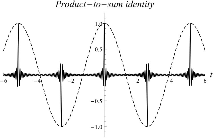 Figure 1
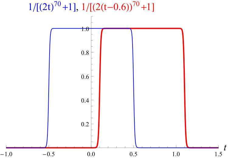 Figure 2
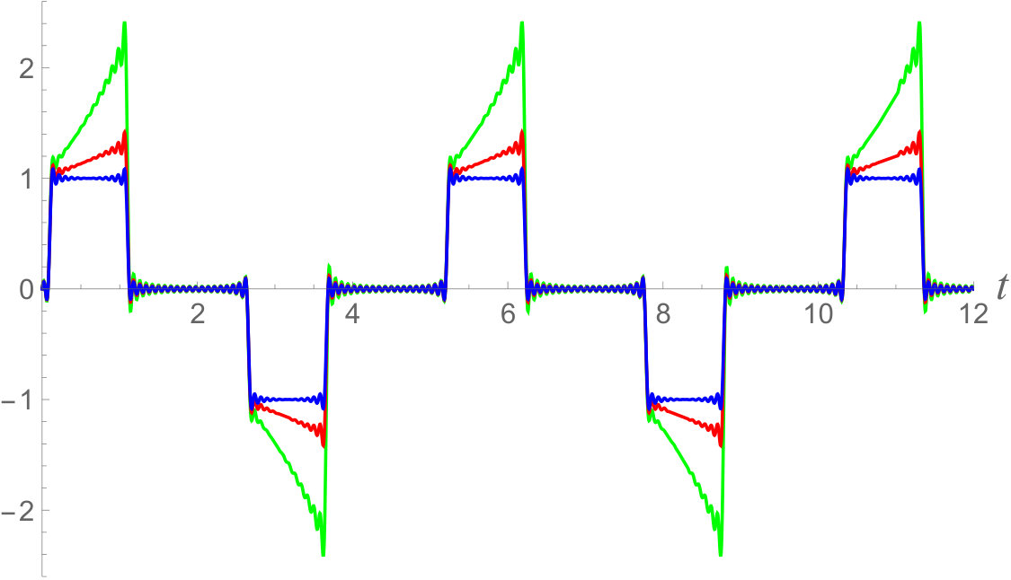 Figure 3
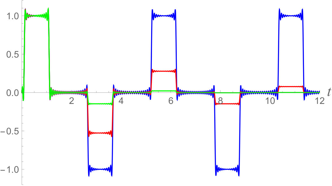 Figure 4
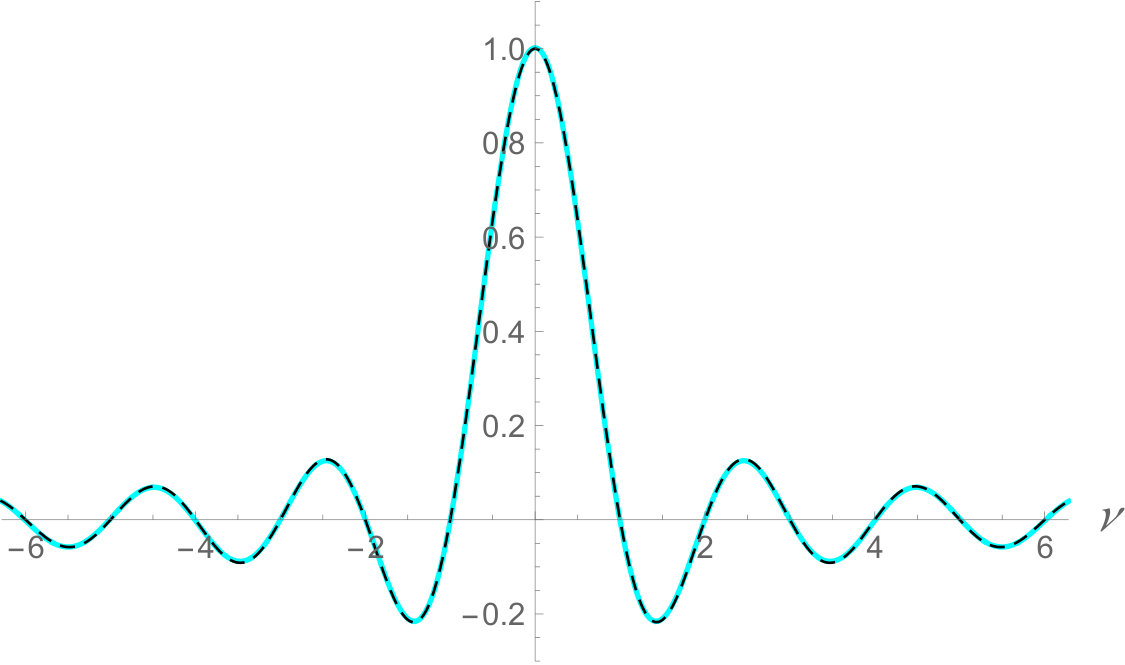 Figure 5
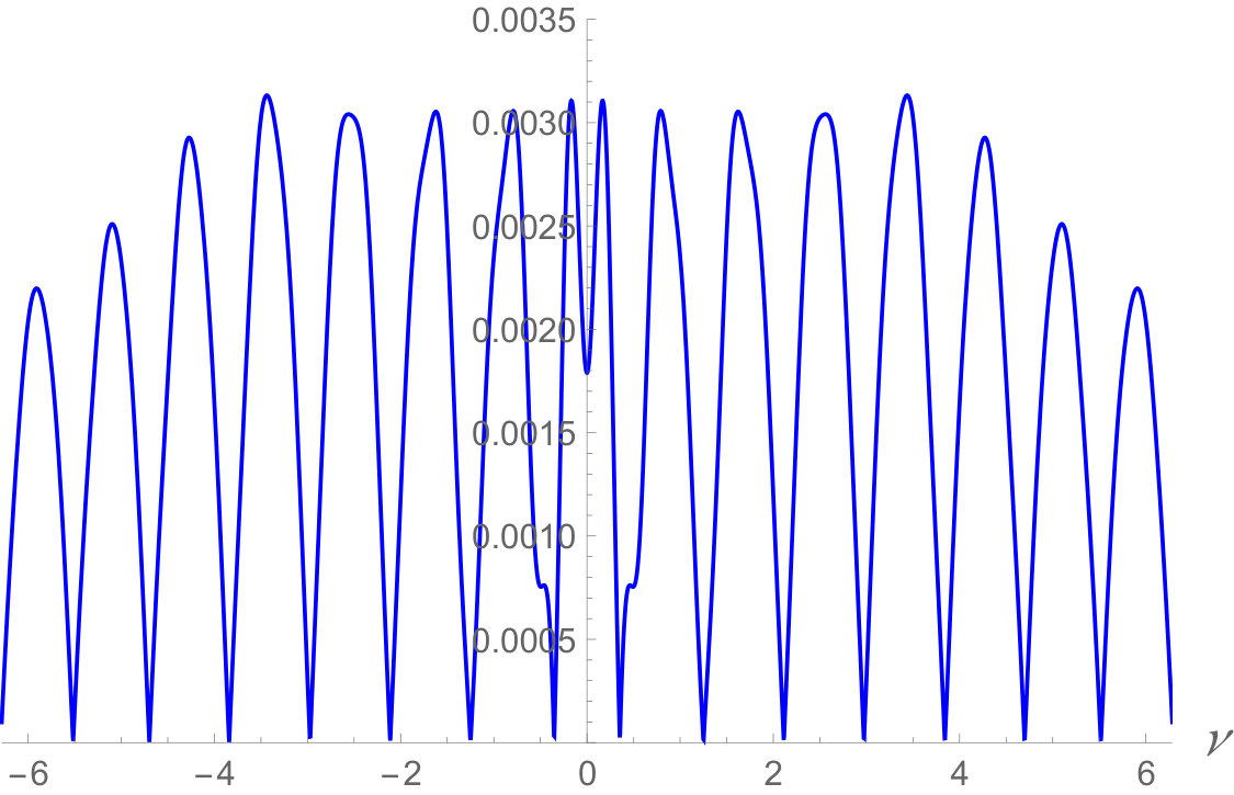 Figure 6
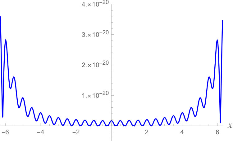 Figure 7
Peer Reviews
No public reviews on file for this paper yet. If you reviewed it on a platform where reviews are public (OpenReview, ICLR, NeurIPS, ICML), you can paste yours below so the community can read it here.
Videos
No videos yet. Explain this paper in a talk, walkthrough, or lecture? Add one.
A rational approximation of the sinc function based on sampling and
the Fourier transforms
S. M. Abrarov111Dept. Earth and Space Science and Engineering, York University, Toronto, Canada, M3J 1P3. and B. M. Quine∗222Dept. Physics and Astronomy, York University, Toronto, Canada, M3J 1P3.
(October 22, 2019)
Abstract
In our previous publications we have introduced the cosine product-to-sum identity [17]
[TABLE]
and applied it for sampling [1, 2] as an incomplete cosine expansion of the sinc function in order to obtain a rational approximation of the Voigt/complex error function that with only summation terms can provide accuracy . In this work we generalize this approach and show as an example how a rational approximation of the sinc function can be derived. A MATLAB code validating these results is presented.
Keywords: sinc function; sampling; Fourier transform; rational approximation; numerical integration
1 Introduction
Sampling is a powerful mathematical tool that can be utilized in many fields of Applied Mathematics and Computational Physics [20, 19, 18]. One of the popular methods of sampling is based on the sinc function that can be defined as [11, 9]
[TABLE]
In particular, any function defined in some interval can be approximated by the following equation (see, for example, equation (3) in [18])
[TABLE]
where are the sampling points, is the small adjustable parameter and is the error term.
The forward and inverse Fourier transforms of function can be defined as [5, 10]
[TABLE]
and
[TABLE]
respectively. In our earlier works we have applied sampling by incomplete cosine expansion of the sinc function and obtained a rapid and highly accurate rational approximation for the Voigt/complex error function that with only summation terms can provide accuracy [1, 2]. As a further development, in this work we generalize the methodology described in our paper [1] by an example showing how sampling and the Fourier transforms (2), (3) can be implemented to obtain a rational approximation of the sinc function.
2 Derivation
The French mathematician François Viète discovered an elegant formula relating the sinc function with cosine infinite product that can be written as given by [11, 9]
[TABLE]
In our earlier publications we have applied the following cosine product-to-sum identity333Initially this identity was reported in our work [17] to resolve a different problem in numerical integration related to the spectrally integrated Voigt function.
[TABLE]
for sampling to expand the Gaussian function for numerical integration [1, 2]. As we can see, the left side of this identity represents a truncated cosine product (4). Consequently, the right side of the identity (5) can be regarded as an incomplete cosine expansion of the sinc function. It is interesting to note that this identity has also found some useful applications in Computational Finance [14, 8, 13]. Here we show how it can also be applied to derive a rational approximation of the sinc function.
Due to product-to-sum identity (5) the sinc function (4) can be rewritten as the following limit
[TABLE]
Consequently, change of the variable in this limit yields
[TABLE]
As we can see now, the truncated form of this limit can be implemented for sampling in accordance with equation (1). Specifically, the sinc function can be approximated as a cosine series expansion such that
[TABLE]
where . Since equation (6) consists of fixed number of the cosine terms, it is, therefore, periodic as it is shown in Fig. 1.
Generally, the sampling grid-points may not be equidistant. However, for simplicity we can assume equidistantly spaced grid-points along -axis. Thus, by taking the substitution of approximation (6) into equation (1) results in
[TABLE]
Similar to equation (6) the right side of equation (7) is also periodic and, consequently, it approximates only within the range .
At the beginning we need to determine the inverse Fourier transform for the sinc function by using equation (3). This leads to
[TABLE]
where
[TABLE]
is commonly known as the rectangular function.
The rectangular function contains two discontinuities at and . Therefore, it is somehow problematic to handle this function due to the high level of oscillation near these discontinuities that occurs as a result of sampling. However, from the well-known relation given by
[TABLE]
where is a positive integer, it follows that the rectangular function can be approximated with high accuracy by taking sufficiently large integer . Thus, if we take, say , then the rectangular function can be approximated very accurately as
[TABLE]
Although this approximation changes very rapidly near the points and , it has no discontinuities and, therefore, can be used for sampling more efficiently then the function itself. Figure 2 shows the function by blue curve.
The function effectively covers the range
[TABLE]
where a small positive value can be taken equal to . By stating “effectively covers the range” we imply that the Fourier transform can be approximated as
[TABLE]
where , since
[TABLE]
and
[TABLE]
are negligibly small and, consequently, can be ignored.
In this approach we consider only the first quadrant. Therefore, we shift the function towards right in form
[TABLE]
as it is shown in Fig. 2 by red curve.
The Fourier transform approximated as
[TABLE]
does not provide a rational approximation as a result of the fixed value on the upper limit of the integration. However, this problem can be effectively resolved by sampling the function instead of as follows444If applicable, the Poisson summation formula can also be used instead of sampling to expand a function of kind . However, the sampling method is more advantageous due to its versatility in practical applications.
[TABLE]
where is a positive (adjustable) number. Figure 3 illustrates the approximation (9) to the function at , , , with , and by blue, red and green curves, respectively.
Since the approximation (9) is periodic, it remains valid only within the range . However, when is big enough, say equal to or greater than , the slight rearrangement of the approximation (9) as given by
[TABLE]
extends the validation of the function along entire positive -axis. This is possible to achieve since the damping multiplier effectively suppresses all peaks (except the first peak near the origin) that appear as a result of this periodicity. This suppression effect given by the damping multiplier can be seen from Fig. 4 that shows the evolution to the function with increasing . In particular, at we observe no suppression and the signal remains periodic (blue curve). However, as increases the suppression effect due to presence of the damping multiplier increases with increasing as shown by red and green curves. Consequently, if the constant is large enough, then the function becomes practically solitary. As a consequence, we can substitute approximation (10) into the equation (8) and replace the upper limit in the integral by practically without loss of accuracy as follows
[TABLE]
Since the upper limit is infinity now the resultant integration yields a rational function. Thus, after some trivial rearrangements that exclude the double summation, from equation (11) it follows that
[TABLE]
where the corresponding expansion coefficients are
[TABLE]
[TABLE]
and
[TABLE]
As we can see, equations (12), (2), (2) and (2) are of the same kind as that of reported in our earlier work [1], where the damping multiplier has also been used in numerical integration for derivation of the rational approximation of the Voigt/complex error function (compare Fig. 4 above with Fig. 3 from our paper [1] to observe same effect of suppression along positive -axis due damping multiplier ).
3 Approximation
Since the function effectively covers the range from [math] to (see red curve in Fig. 2), it is not necessary to run the index starting from . Therefore, the expansions (2) and (2) can be slightly modified by running the index from [math] to . This leads to
[TABLE]
and
[TABLE]
Using the shifting property of the Fourier transform (2) we can write
[TABLE]
Consequently, from equations (12) and (14) we obtain
[TABLE]
Figure 5 shows a rational approximation (15) of the sinc function by light blue curve. The black dashed curve shows the original sinc function for comparison. As we observe, the original sinc function and its rational approximation (15) are not distinctive visually.
Figure 6 shows the absolute difference between the original sinc function and its rational approximation. Despite that the sinc function is not easy to approximate [16, 12], only terms in the proposed formula (15) provide absolute difference smaller than within the range . A MATLAB code validating the results based on the rational approximation (15) of the sinc function is provided in Appendix A. Specifically, a command line rationapp(1) displays two graphs with approximated sinc function and its absolute difference.
It should be noted that significantly higher accuracy can be achieved with more well-behaved functions. For example, substituting the function into equation (15) and taking parameters , , , and we can obtain a rational approximation of the function with absolute difference less than . This can be readily confirmed by running a MATLAB code provided in Appendix A. In particular, a sample computation that can be run by a command line rationapp(2) shows that the absolute difference between original function and its rational approximation does not exceed .
4 Numerical integration
The application of the rational approximation (15) may be especially advantageous for a contour integral of kind
[TABLE]
where is a multivariable function, since it may be computed numerically by residues when the integrand on the right side of integral in equation (16) is analytic. This is possible to achieve due to presence of the poles in the rational approximation of function . For example, applying the functions
[TABLE]
and
[TABLE]
in equation (16), the following integral
[TABLE]
known as the Voigt function [3], can be calculated by residues in a similar way that we performed in our earlier work [2] to approximate the integral (17). Due to rapid performance and high accuracy our algorithm [2] has been implemented in current version of the atmospheric model bytran [15, 6]. Thus, integration by residues leads to
[TABLE]
This approximation can provide highly accurate values as we can see from the Fig. 7 showing an example of the absolute difference between the original Voigt function and its approximation (18). In particular, a computation performed with extended precision floating-point by using Wolfram Mathematica (version 11) shows that at , , , , and the absolute difference does not exceed within the range (see also Appendix B showing how else the Voigt function can be computed).
This integration method may be promising in computation of the more sophisticated functions, known as the Voigt function moment integrals, that are used in the atmospheric radiative transfer model MODTRAN [4]. Our preliminary results show that it can also be efficient in derivation of the rapid and accurate approximation series for some of the integrals involving the Gaussian function reported in the recent paper [7].
5 Conclusion
We generalize a methodology shown in our earlier publication [1] and show as an example how to derive a rational approximation of the sinc function by sampling and the Fourier transforms. Despite that the sinc function is not easy to approximate, our results reveal that with only summation terms the absolute difference between the sinc function and its rational approximation does not exceed within the range .
Acknowledgments
This work is supported by National Research Council Canada, Thoth Technology Inc. and York University. The authors wish to thank the Reviewers for constructive comments and recommendations. Useful remarks and suggestions from John M. Campbell (York University) are greatly appreciated.
Appendix A
function rationapp(opt)
% This function file computes a rational approximation of the sinc and % v*exp(-(v)^2) functions by using equation (16).
if nargin == 0 opt = 1; % choose option 1 if argument is missing disp(’Missing input parameter! Option opt = 1 is assigned.’) end
switch opt case 1 % Define parameters a = 0.6; k = 35; sigma = 2.7; M = 6; h = 0.04; N = 28;
    n = 0:N; % define array n

    f = 1./((2*(h*n - a)).^(2*k) + 1); % function f(t - a)
    % f = exp(-(2*(n*h - a)).^(2*k)); % alternative function f(t - a)

    func = ’sinc(nu)’; % string for first function
    str = ’Sinc approximation’; % string for y-label

case 2
    % Define parameters
    a = 2;
    sigma = 5;
    M = 6;
    h = 0.078;
    N = 55;

    n = 0:N; % define array n

    f = pi^(3/2)*1i*(n*h - a).*exp(-(pi*(n*h - ...
        a)).^2); % function f(t - a)

    func = ’nu.*exp(-(nu).^2)’; % string for second function
    str = ’Approximation {\it{\nu e^{-\nu^2}}}’;  % string for y-label

otherwise
    disp([’Parameter ’,num2str(opt),’ is wrong! Choose eather 1 or 2.’])
    return
end
m = exp(sigmanh); % exponential multiplier fm = f.*m; M2=2^(M-1);
% Define column arrays alpha = zeros(M2,1); beta = zeros(M2,1);
% Compute the expansion coefficients % Equations (13c), (14a) and (14b) gamma=pi*(2*[1:M2]’-1)./(2^Mh); for m = 1:M2 alpha(m) = 1/M2sum(fm.cos(gamma(m).nh),2); beta(m) = 1/M2sum(fm.*gamma(m).*sin(gamma(m).nh),2); end
%-------------------------------------------------------------------------- % APPROXIMATION (16) %-------------------------------------------------------------------------- nu = linspace(-2pi,2pi,1000); % define array for the argument nu funcApp = 0; % initiate function approximation as zero
for m=1:M2 funcApp = funcApp + (alpha(m)(sigma + 2pi1inu) + ... beta(m))./(gamma(m)^2 + (sigma + 2pi1inu).^2); end funcApp = exp(2pi1inu*a).*funcApp; % final result %--------------------------------------------------------------------------
% FIGURE 1 figure1 = figure; axes1 = axes(’Parent’,figure1,’FontSize’,12); xlim(axes1,[-2pi,2pi]); box(axes1,’on’); grid(axes1,’on’); hold(axes1,’all’); plot1 = plot(nu,[real(funcApp);eval(func)],’Parent’,axes1); set(plot1(1),’LineWidth’,3,’Color’,[0 1 1]); set(plot1(2),’LineStyle’,’--’,’LineWidth’,2); xlabel(’Parameter \it{\nu}’,’FontSize’,14); ylabel(str,’FontSize’,14);
% FIGURE 2 figure2 = figure; axes2 = axes(’Parent’,figure2,’FontSize’,12); xlim(axes2,[-2pi,2pi]); box(axes2,’on’); grid(axes2,’on’); hold(axes2,’all’); plot2 = plot(nu,abs(eval(func) - real(funcApp)),’Parent’,axes2); set(plot2(1),’LineWidth’,1,’Color’,[0 0 0]); xlabel(’Parameter \it{\nu}’,’FontSize’,14); ylabel(’Absolute difference’,’FontSize’,14);
Appendix B
Due to symmetric forms of the equations (2) and (3) an approximation for the inverse Fourier transform follows immediately from the equation (15) as
[TABLE]
where the expansion coefficients can be found accordingly as
[TABLE]
and
[TABLE]
Therefore, the Voigt function (17) can also be computed by using the contour integral of kind
[TABLE]
such that the functions are and
[TABLE]
The reference list from the paper itself. Each links out to its DOI / PubMed record.
- 1[1] S.M. Abrarov and B.M. Quine, Sampling by incomplete cosine expansion of the sinc function: Application to the Voigt/complex error function, Appl. Math. Comput., 258 (2015) 425-435. http://dx.doi.org/10.1016/j.amc.2015.01.072 · doi ↗
- 2[2] S.M. Abrarov and B.M. Quine, A rational approximation for efficient computation of the Voigt function in quantitative spectroscopy, J. Math. Res., 7(2) (2015) 163-174. http://dx.doi.org/10.5539/jmr.v 7n 2 · doi ↗
- 3[3] B.H. Armstrong, Spectrum line profiles: The Voigt function, J. Quant. Spectrosc. Radiat. Transfer, 7(1) (1967) 61-88. https://doi.org/10.1016/0022-4073(67)90057-X · doi ↗
- 4[4] A. Berk, Voigt equivalent widths and spectral-bin single-line transmittances: Exact expansions and the MODTRAN ® 5 implementation, J. Quant. Spectrosc. Radiat. Transfer, 118 (2013) 102-120. https://doi.org/10.1016/j.jqsrt.2012.11.026 · doi ↗
- 5[5] R.N. Bracewell, The Fourier transform and its applications, 3rd ed., Mc Graw-Hill, 2000.
- 6[6] bytran − | − -\left|\right.- spectral calculations for portable devices using the HITRAN database. http://www.bytran.org/
- 7[7] C. Chesneau and F. Navarro, A note on simple approximations of Gaussian type integrals with applications (2018). hal-01888264
- 8[8] G. Colldeforns-Papiol, L. Ortiz-Gracia, Computation of market risk measures with stochastic liquidity horizon, J. Comput. Appl. Math., 342C (2018) 431-450, https://doi.org/10.1016/j.cam.2018.03.038 · doi ↗