Quantum cosmology of Bianchi VIII, IX LRS geometries
A. Karagiorgos, T. Pailas, N. Dimakis, G. O. Papadopoulos, Petros A., Terzis, T. Christodoulakis

TL;DR
This paper revisits Bianchi VIII and IX cosmological models, deriving classical solutions using integrals of motion and exploring quantum solutions via the Wheeler DeWitt equation, with implications for understanding collapsed configurations.
Contribution
It introduces a novel method using quadratic integrals of motion and homothetic vectors to analyze classical and quantum Bianchi models.
Findings
Classical solutions derived using new integrals of motion.
Quantum solutions obtained from Wheeler DeWitt equation with two operators.
A probabilistic interpretation that excludes collapsed configurations.
Abstract
In the present work we revisit the axisymmetric Bianchi VIII and IX models. At the classical level we reproduce the known analytic solution, in a novel way making use of two quadratic integrals of motion, the constraint equation, as well as a linear non-local integral of motion. These quantities correspond to two second rank Killing tensors and a homothetic vector field existing on the relevant configuration space. On the corresponding phase space the two quadratic charges commute with the Hamiltonian constraint but not among themselves. Thus, after turning these charges into operators we obtain two different solutions to the Wheeler DeWitt equation utilizing each of the quadratic operators. The homothetic vector is then used, as a natural guide line, to define a normalizable conditional probability which assigns zero to the classically collapsed configurations.
Click any figure to enlarge with its caption.
 Figure 1
 Figure 2
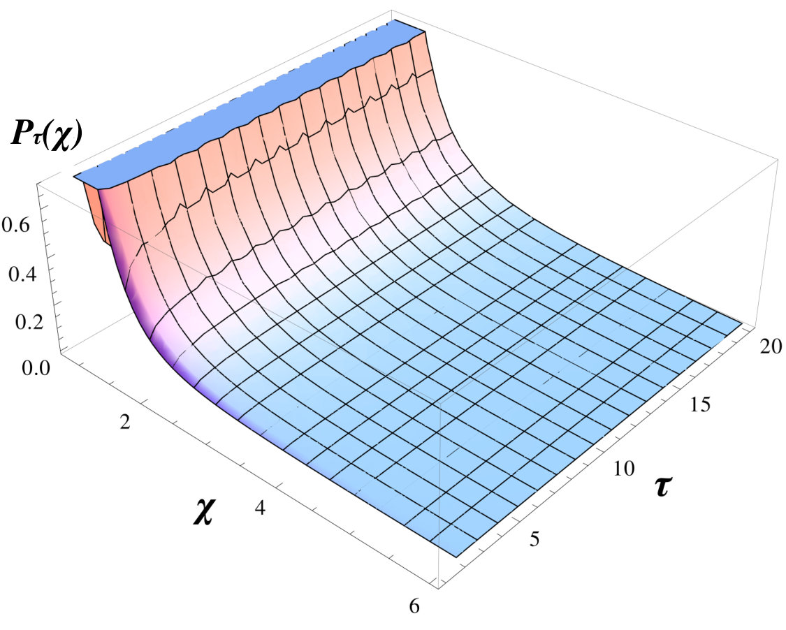 Figure 3
 Figure 4
Peer Reviews
No public reviews on file for this paper yet. If you reviewed it on a platform where reviews are public (OpenReview, ICLR, NeurIPS, ICML), you can paste yours below so the community can read it here.
Videos
No videos yet. Explain this paper in a talk, walkthrough, or lecture? Add one.
Quantum cosmology of Bianchi VIII, IX LRS geometries
A. Karagiorgos
T. Pailas
N. Dimakis
G.O. Papadopoulos
Petros A. Terzis
T. Christodoulakis
Abstract
In the present work we revisit the axisymmetric Bianchi VIII and IX models. At the classical level we reproduce the known analytic solution, in a novel way making use of two quadratic integrals of motion, the constraint equation, as well as a linear non-local integral of motion. These quantities correspond to two second rank Killing tensors and a homothetic vector field existing on the relevant configuration space. On the corresponding phase space the two quadratic charges commute with the Hamiltonian constraint but not among themselves. Thus, after turning these charges into operators we obtain two different solutions to the Wheeler DeWitt equation utilizing each of the quadratic operators. The homothetic vector is then used, as a natural guide line, to define a normalizable conditional probability which assigns zero to the classically collapsed configurations.
1 Introduction
A first approach to Bianchi IX cosmological model has been initiated by Misner [1], Ryan [2] and Belinskii, Khalatnikov and Lifshitz (BKL) [3, 4]. In these works use has been made of the well known Misner variables , where is the scale factor measuring the overall volume of the spatial slice, while and its anisotropy. The system can be interpreted as a particle moving in a time-dependent potential well. Dynamical and numerical studies have been performed for its trajectory implying a possible chaotic behaviour [5, 6, 7, 8, 9]. The fully anisotropic model created great debate in the literature regarding its integrability and whether - and in which sense - it exhibits chaos, we refer the interested reader to some basic works concerning these matters [10, 11, 12, 13, 14, 15, 16, 17, 18, 19, 20, 21]. On the other hand, the Bianchi type VIII model has not attracted the same level of interest in the literature as has the type IX with its closed hypersurfaces. However, there exist interesting studies and exact solutions that have been derived [22, 23, 24].
It is widely known that for specific classes of spatially homogeneous space-times [25] the principle of symmetric criticality [26, 27] holds, i.e. a reduced action that results from the space-time symmetries can be used to generate correctly the equations of motion of the model, i.e. those obtained by imposing the symmetry requirement at the level of Einstein’s Field Equations. The emanating Lagrangian possesses a finite number of degrees of freedom and it is the basis of the so called mini-superspace description. There have been a lot of studies making use of this property especially in what regards the symmetries that the reduced system possesses [28, 29, 30, 31, 32, 33, 34, 35, 36, 37]. This procedure is of special interest in what regards the quantization of the reduced system, since this can give a hindsight of what one could expect from the quantum version of the gravitational configuration. This gave rise to the field of quantum cosmology [38, 39, 40, 41, 42, 43, 44, 45, 46, 47]. Both Bianchi types VIII and IX admit such a description.
In the present work we have, at the classical level, re-acquired the solution to the Einstein’s equations for the empty axisymmetric Bianchi Types VIII, IX model. The novelty is that, in order to find the solutions, we utilize the constants of motion inferred from the corresponding mini-supermetric, i.e. the conserved (local) charges produced by two Killing tensor fields (second rank) and a non-local corresponding to a homothetic Killing vector field (first rank), along with the quadratic constraint. A similar approach has been recently adopted for Bianchi IX plus a cosmological constant [48]. The difference here is that the empty classical case has one more second rank symmetry.
At the quantum level, we turn the quadratic charges into operators which commute with the quadratic constraint operator (defining the Wheeler-DeWitt equation) but not among themselves. We thus obtain, using each of the quantum charges as subsidiary condition on the wave function, two distinct quantum states (modulo integration constants). We show that, with the help of the homothetic vector, a conditional probability can be defined which assigns zero to the classically collapsed configuration.
The structure of this paper is as follows: In section 2 we present the minisuperspace of axisymmetric Bianchi VIII, IX models, study its symmetries and, through them, obtain the classical solutions. In section 3 we study the quantization of the model. Section 4 contains our analysis on the choice of an internal time variable with the help of the homothetic symmetry of the mini-superspace metric. Finally, in the last section we give our conclusions.
2 Mini-superspace for axisymmetric Bianchi VIII and IX model
For the general Bianchi models VIII and XI, a generic scale factor matrix can be diagonalized solely through kinematics and then the use of linear constraints dictates the vanishing of the shift vector (see e.g. [49, 50]). In the present work we focus in the case of axisymmetry; our starting point is, thus, the line element
[TABLE]
with (note that the alternative choices turn out to be incompatible for VIII [51, 50]) and the one-forms corresponding to Bianchi VIII, IX symmetry group are given by
[TABLE]
with and for Bianchi VIII and Bianchi IX respectively.
The Ricci scalar for this metric is
[TABLE]
It is well known that the reduced Einstein Hilbert action provides the correct dynamics i.e. the inferred Lagrangian is valid. In order to enclose the entire dynamics in the kinetic part, and also simplify our calculations, we rescale the lapse as which effectively makes the potential independent of and ; the final form of the Lagrangian is therefore given by
[TABLE]
For the sake of simplicity we adopt, in what follows, the change to light-cone coordinates
[TABLE]
Thus, the transformed Lagrangian and its corresponding mini-supermetric are written as
[TABLE]
[TABLE]
The above Lagrangian is singular and applying the Dirac-Bergmann [52, 53] algorithm for constrained systems we obtain the weakly vanishing Hamiltonian constraint
[TABLE]
with . In order to reproduce the classical solution we can use possible extra symmetries of the above configuration space. The mini-supermetric has both first and second order symmetries. Of the first kind there is only one homothetic vector field and of the second there are two second rank Killing tensor fields; overall we have
First-order:
[TABLE]
Second-order:
[TABLE]
[TABLE]
It has been shown in [31, 54] that proper homothetic or conformal Killing vectors of the mini-superspace metric can be used to define non-local conserved charges that involve an explicit time dependence in the form of an integral of phase-space variables. In this particular case, the non-local conserved quantity generated by is
[TABLE]
It is easy to verify that the total derivative of the above expression vanishes on mass shell. At the same time, the two Killing tensors define of course the following local integrals of motion
[TABLE]
[TABLE]
The above conserved quantities are more than enough for the acquisition of the classical solution. What is more, the latter can be derived by purely algebraic means. Note that this is possible only because the non-local charge gives non trivial time dependence to the algebraic solution obtained when the four charges are solved for . Thus, combining together and we arrive at the solution. For the non-local conserved charge it is enough to require instead of constant because it involves an indefinite integral in its expression. This system of equations result into two different branches for the solution depending on whether the value of is zero or non-zero.
2.1 Case with
The general system of equations under consideration is the following
[TABLE]
where (2.16) has been obtained from expressed in terms of velocities. At first we solve the constraint for and replace into the two equations (2.17) and (2.18). The result is the following set of equations
[TABLE]
where with is the term . We can now solve the equations (2.20b,2.20c) algebraically with respect to the velocities . If this solution is substituted into eq. (2.20a), a purely algebraic relation among is obtained:
[TABLE]
Furthermore, eq. (2.20b) being an 1-form in 2D is necessarily closed, and thus can be written in the form defining one more algebraic relation between
[TABLE]
Since, we have not used any choice of time these two relations are not independent and define one relation between , namely
[TABLE]
The lapse is given from the constraint equation as
[TABLE]
It can be seen that the last two expressions satisfy the Euler-Lagrange equations of Lagrangian (2.8). Thus, the final form of the solution (given in terms of the initial variables ) can be expressed in the time gauge as
First branch.
We write
[TABLE]
where we have set . In order to not have a signature change and keep and positive, the variable has to be restricted appropriately by the constants and . For example:
- •
In the case one must require that
[TABLE]
- •
On the other hand, if then the following inequalities must hold
[TABLE]
Second branch.
In this case we have the square root appearing with the opposite sign
[TABLE]
The requirement of positive and leads to the conditions:
- •
If , then you may have either
[TABLE]
or
[TABLE]
- •
In the other case where we are led to
[TABLE]
or
[TABLE]
The number of the constants appearing in the solutions is exactly what is expected due to the axisymmetry assumption: (number of independent scale factors)-(number of first class constraints). Both of them are essential as it can be seen by the fact that the Wronskian matrix , where ’s are the four dimensional scalar curvatures (, , ) and , has ; which means that can be expressed as functions of ’ s.
2.2 Special case with
In this case the system of equations under consideration is simpler. Again we follow the same procedure by solving algebraically eqs. (2.20b) and (2.20c) with respect to the velocities and , where in the former we have st of course . The substitution into (2.20a) yields the following simplified relation between and
[TABLE]
The final solution can be neatly expressed in terms of without any particular choice of time:
[TABLE]
which, when , we observe that it is a solution of Lorentzian signature if . On the other hand, in the case we see that the signature is , indicating a shift of roles between coordinates. When the opposite situation occurs. The constant is essential for the corresponding geometries.
As a preparation for the quantum case we next investigate all the Abelian Poisson Bracket subalgebras formed by the quadratic charges and the Hamiltonian. Since the Poisson bracket of and is non-zero the only remaining possibilities are
[TABLE]
We can thus hope for two different quantum states which will correspond to the quantum analogues of either and or and .
Lastly, a word about the linear homothetic charge is pertinent: Its non-local character excludes any use of the corresponding quantum analogue in the entire configuration space. Of course, if one wanted to indulge into the reduced phase space where the “true” Hamiltonian governs the dynamics, then the nonlocal linear integral would be an ideal candidate for the time variable to be factored out along with the conjugate momenta; thus arriving at a Schrödinger-like wave equation for .
3 Quantum solutions
It is well known that the quantum analogue of the Hamiltonian constraint i.e. the Wheeler-DeWitt(WDW) equation does not in most cases suffice to determine the wave function up to an additive constant phase; yet this is an essential requirement in the context of quantum mechanics. Fortunately, in the presence of further symmetries, one can supplement the WDW equation with the eigenvalue equations constructed out of the quantum analogues of the symmetry generators. In the canonical analysis the first step is to assume the mapping
[TABLE]
between Poisson brackets and the commutators. A way for this o be realized is by assigning differential operators to momenta
[TABLE]
while the positions are considered to act multiplicatively. In order to resolve the factor ordering problem of the Kinetic term of , we choose the conformal Laplacian (or Yamabe operator),
[TABLE]
where , , is the Ricci scalar and the dimension of the mini-superspace. Moreover, classical symmetries produced by linear vector and Killing tensor fields are naturally transcribed at the quantum level by assigning to the general expression for linear first order, Hermitian operators [55] and to a psedo-Laplacian operator [56]; thus the corresponding forms are respectively
[TABLE]
[TABLE]
In our case the linear homothetic symmetry produces a non-local charge and thus it is not immediately usable in the four-dimensional phase space , spanned by . Therefore, we turn to the quadratic charges produced by the two Killing tensors: one can easily verify that the relevant commutators are zero
[TABLE]
Note that the above relations hold for any irrespectively of whether it solves the Hamiltonian constraint or not. We thus distinguish the two Abelian quantum sub-algebras and .
Sub-algebra
These operators give the following set of eigenvalue equations for the wave function
[TABLE]
[TABLE]
[TABLE]
[TABLE]
where is the constant appearing in the classical solution. As a first step in the solution procedure, we solve the Hamiltonian constraint with respect to , and replace into (3). In order to make the final equations simpler and create a separable set of equations we use the transformation
[TABLE]
thus ending up with the following set of equations
[TABLE]
[TABLE]
The general solution to the above system is
[TABLE]
with
[TABLE]
[TABLE]
where and are integration constants. The coupling constant appearing in (3.8) and (3.8) has been fixed by the quadratic constraint relation at the value .
Sub-algebra
The corresponding equations emerge from the quantum Hamiltonian constraint given by (3.5) and the action of on the wave function
[TABLE]
[TABLE]
Once more we solve (3.5) with respect to , and substitute into the above equation, which is then reduced to
[TABLE]
with the following general solution:
[TABLE]
The form of and is determined by substituting the above expression for into equation (3.5) and, in the resulting equation, setting to zero the coefficients of the above sin and cos . The final result is given by
[TABLE]
where , are integration constants.
4 Interpretation through Homothetic time
Once we have secured the existence of quantum states defined up to constants, we now must turn to the question of their interpretation. This is a well known, difficult problem in quantum cosmology (for a comprehensive review of the various approaches see e.g. [57, 58]). The main problem is the reparametrization invariance of the classical theory which is transcribed at the quantum level through the Wheeler DeWitt equation.
In the usual quantum mechanics normalizability of the states is expected by integration over the configuration space variables but not over time. The problem which arises in quantum cosmology is that any combination of the configuration space variables, say in our case, must be allowed to be considered as time; consequently, in the definition of probability we must take into account this fact. In this respect two main approaches have been developed.
One consists in selecting the combination which is to represent time before quantization, thus arriving at a reduced phase space where the dynamics is governed by the ”true” Hamiltonian through a Schrödinger like equation (see e.g. [59, 60]). In the present case this would ideally fit with the use of the existing homothetic vector and it’s conjugate to define time and energy.
The second scheme involves a selection of time after the quantization has been performed and the subsequent definition of a conditional probability on the complementary configuration space. In both approaches a really serious problem is the justification of the particular choice of time employed. It is natural to seek this justification in existing classical structures of the configuration manifold.
In what follows we adopt the second point of view. Since the two quadratic charges have already been used in the previous section for the derivation of our solutions, it is reasonable to turn to the linear homothetic charge for a justification of the choice for time.
Given that the dimension of the configuration space is two, the corresponding to one form is necessarily closed, and we thus expect that it can be brought into the form
[TABLE]
Indeed, it is straightforward to verify that the correct expressions are:
[TABLE]
Our proposal is now to select as natural time variable the quantity . Thus, the orthonormal coordinate system is composed by the following two variables
[TABLE]
in which the transformed minisuperspace metric is diagonal
[TABLE]
with a corresponding Ricci scalar . We see that there are curvature singularities of the configuration manifold described by in the model and by for the model. If we notice that, in the initial variables , and take into account the classical solutions, we conclude that corresponds to the 4-dim space-time curvature singularity, while is never attained on the classical orbits. This singularity is brought in our configuration space geometry by the rescaling of the initial lapse and thus corresponds to the vanishing of the Ricci scalar of the three dimensional spatial slice; thus never occurring for the considered models. Therefore, the range of integration for the variable will be initially taken when defining the conditional probability.
The probability density is defined using the natural measure
[TABLE]
as
[TABLE]
If the integral over of the above function converges, say to some , then we can define the conditional probability of the quantum state of the universe to be in the configuration interval as
[TABLE]
Let us now apply this reasoning to the case of the second algebra. There are two separate regions depending on the value of into the exponential function being positive or negative. The ensuing state is normalizable in the above conditional probability density; since .
4.1 Second solution
The second algebra yields solution (3.16), which in the variables reads
[TABLE]
In the first case
we consider that and the solution has a decay form. The wave function is in this case
[TABLE]
where, for the sake of normalizability, we have kept only the term which vanishes when tends to zero. Therefore, the probability density is
[TABLE]
which tends to zero for and for for Bianchi type IX.
In the second case
; now both terms oscillate. We consider the positive frequency mode since we want only outgoing waves. Thus, by setting and . the wave function becomes
[TABLE]
The above defined is given by
[TABLE]
whose existence and finite behaviour is guaranteed by the inequality for this case. The corresponding conditional probability density is
[TABLE]
which vanishes for the classically collapsed configurations designated by . In figure (1) we plot the normalized probability density with respect to and . Note that the depicted ranges for and are those allowed by the basic inequality above assumed.
4.2 First solution
In this case the wavefunction is given by (3.10) which expressed in variables reads
[TABLE]
where we have absorbed the Gamma functions into the constants .The situation is considerably more involved since products of the Bessel functions appear in every term of . We only give the limitations on imposed by the demand of normalizablity: The only dangerous point is at with fixed , where the arguments become small and tend to zero. Both and are problematic at zero if is negative while at the same time not an integer, thus . For the other values , unless for which .
If then is real and distinct approaches can be followed:
- (a)
Eliminate the branches of the solution that have a negative index by setting and have a wave function
[TABLE] 2. (b)
Keep both branches, but restrict so that . However, in this case, and seize to be independent since when is an integer. The same is also true for the and when , . Thus, we end up again with the same wave function as in case 1a, but with a different condition on .
[TABLE] 2. 2.
If then the indexes are imaginary, , . The resulting Bessel functions are bounded, but the limit at zero cannot be calculated. It is a limit of the form
[TABLE]
it fluctuates on the complex plane. However, whatever one might choose here the wave function is going to be bounded as .
Thus, given the above described allowed values for the indexes the would be finite and a similar qualitative analisis to the previous case will hold.
5 Discussion
In the present work we have studied the mini-superspace models of Bianchi type VIII and IX LRS geometries.
At the classical level we have reproduced the solution space through the use of the symmetries of the configuration space manifold. Specifically, these symmetries consist of a homothetic killing and to second order killing tensor fields. Together with the Hamiltonian constraint these four charges, when expressed in velocity phase space, provide an algebraic system for the two positions and the corresponding velocities; its solution is enough to reveal the entire solution space of the problem. Except the well known solutions (2.25) and (2.28), the solution (2.34) is,to the best of our knowledge, new. When , it exhibits the interesting phenomenon of signature change as spans the interval .
At the quantum level we have followed the canonical quantization method. In order to determine a unique (up to constants) wave function, we have used-except the Wheeler-DeWitt constraint equation- the operators corresponding to Abelian subalgebras formed by the two pairs consisting of the before-said constraint and each of the two operators corresponding to the quadratic symmetry generators.
The linear non-local charge has been used as a guideline for selecting a natural physical time in the configuration space and thus define a conditional probability with respect to which the classically singular configurations are assigned zero weight.
Last, but not least, we would like to discuss the existence of the notion of homothetic time adopted in this work. At first glance, one might think that this is particular to the situation depicted in the present work, i.e. the fact that we have a two dimensional configuration space; as a consequence every one- form is necessarily closed and therefore the same is true for the one-form corresponding to the homothetic vector. In fact this is not the case: the homothetic vector exists(as the only linear symmetry generator) even for the totally anisotropic case with ; what is more important the corresponding one form is also closed. Thus, the described procedure of defining the conditional probability adopted in this work will also be valid in this case as well. The same reasoning holds true even for a full scale factor matrix : the corresponding Langrangian density is , where , is the usual extrinsic curvature of the slice constant, is its Ricci scalar, , and we have redefined the usual lapse as so that the vector is revealed as a homothecy generator for the scaled mini-supermetric . One can be satisfied that the corresponding one form is again closed. This may well be the starting point of future work.
Acknowledgments
The research work was supported by the Hellenic Foundation for Research and Innovation (HFRI) and the General Secretariat for Research and Technology (GSRT), under the HFRI PhD Fellowship grant (GA.no.74136/2017).
The reference list from the paper itself. Each links out to its DOI / PubMed record.
- 1[1] C. W. Misner, Phys. Rev. Lett. 22 , (1969) 1071
- 2[2] Ryan, Michael P., Annals of Physics 70.2 (1972): 301-322.
- 3[3] V. A. Belinskii, and I. M. Khalatnikov, Sov. Phys. JETP 29.5 (1969): 911-917.
- 4[4] V. A. Belinskii, and I. M. Khalatnikov, and E. M. Lifshitz. Advances in Physics 19.80 (1970): 525-573.
- 5[5] A. R. Moser, R. A. Matzner and M. P. Ryan Jr., Ann. Phys. 79 , (1973) 558
- 6[6] B. Berger, Class. Quant. Grav 7, 203 (1990).
- 7[7] B. K. Berger, Phys. Rev. D 49 , (1994) 1120
- 8[8] B. K. Berger, D. Garfinkle and E. Strasser, Class. Quantum Grav. 14 , (1997) L 29-L 36