Complex Networks in the Framework of Nonassociative Geometry
Alexander I. Nesterov, Pablo H\'ector Mata Villafuerte

TL;DR
This paper introduces a nonassociative geometric model for complex networks, effectively capturing the small-world property and providing insights into Internet structure and other real-world networks.
Contribution
It presents a novel nonassociative geometric framework that extends statistical models of complex networks, successfully explaining empirical Internet data.
Findings
Model accurately reproduces Internet connectance data
Nonlocal curvature controls small-world properties
Applicable to various complex networks
Abstract
In the framework of on nonassociative geometry, we introduce a new effective model that extends the statistical treatment of complex networks with hidden geometry. The small-world property of the network is controlled by nonlocal curvature in our model. We use this approach to study the Internet as a complex network embedded in a hyperbolic space. The model yields a remarkable agreement with available empirical data and explains features of Internet connectance data that other models cannot. Our approach offers a new avenue for the study of a wide class of complex networks, such as air transport, social networks, biological networks, etc.
Click any figure to enlarge with its caption.
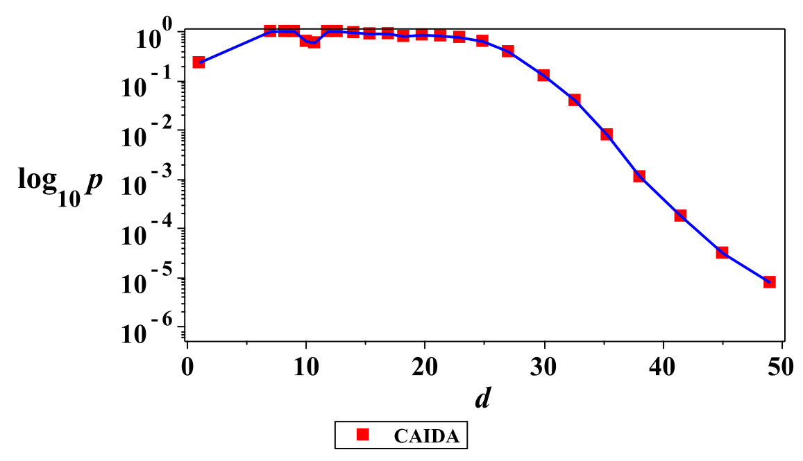 Figure 1
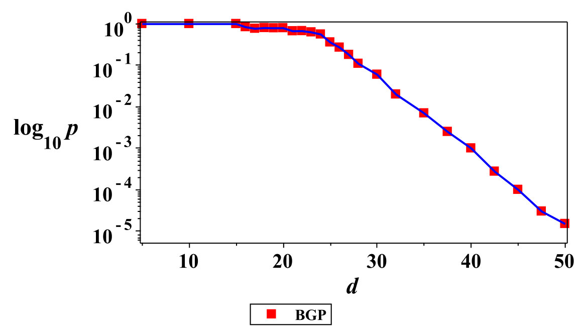 Figure 1
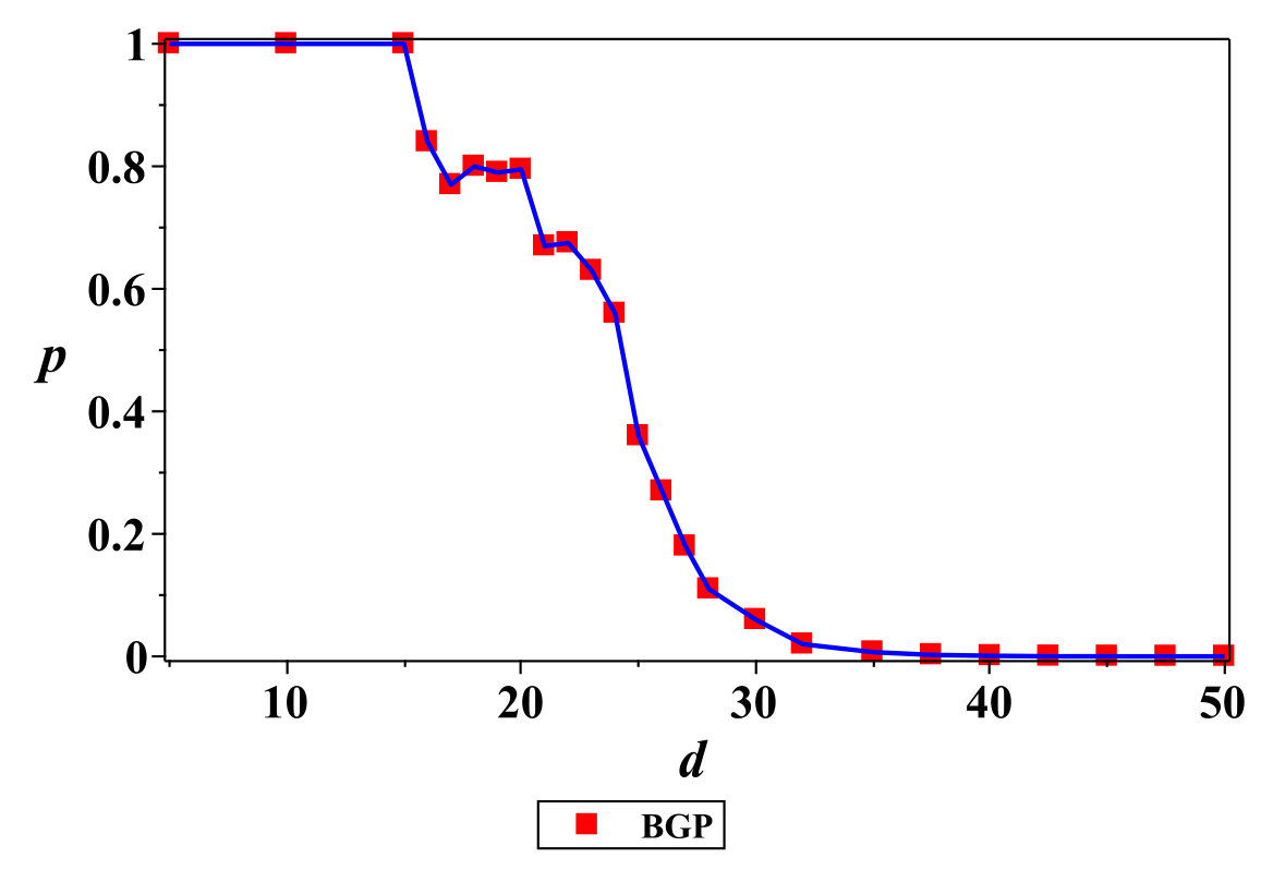 Figure 1
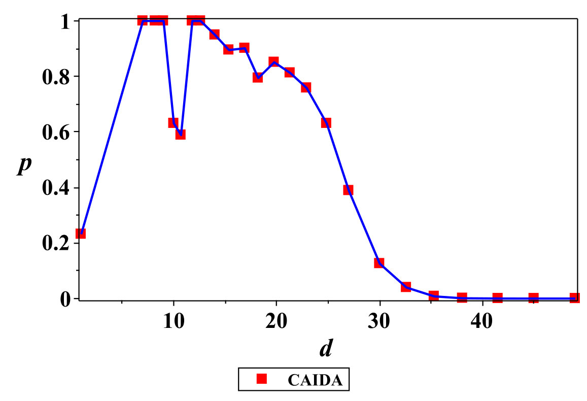 Figure 1
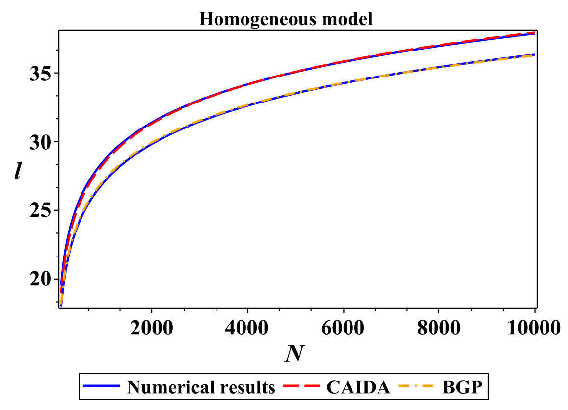 Figure 10
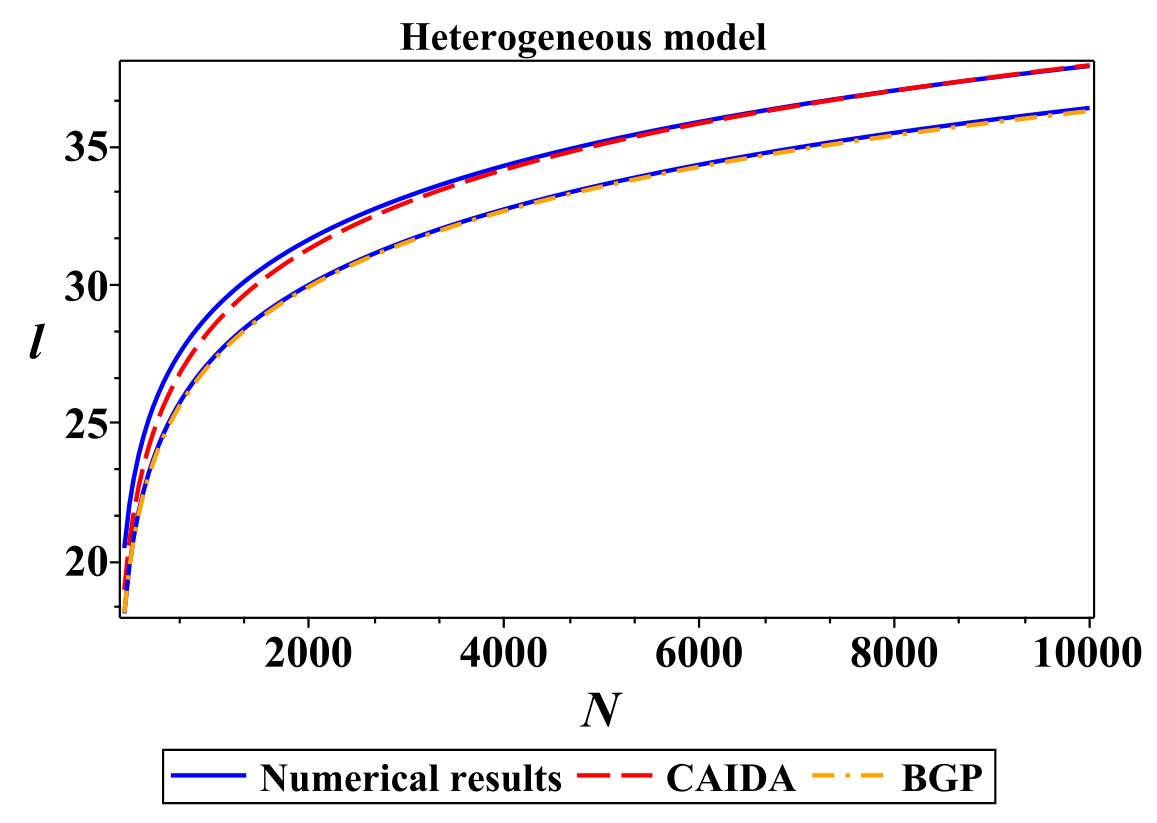 Figure 10
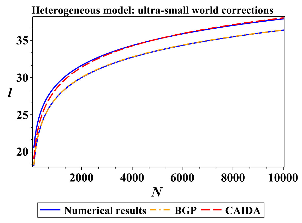 Figure 10
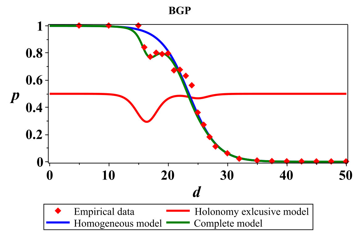 Figure 12
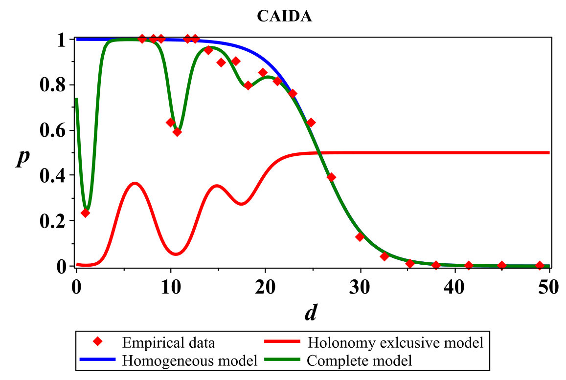 Figure 12
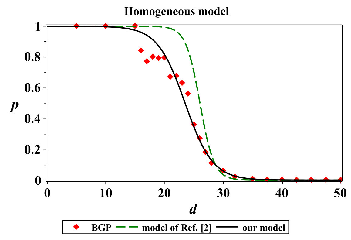 Figure 2
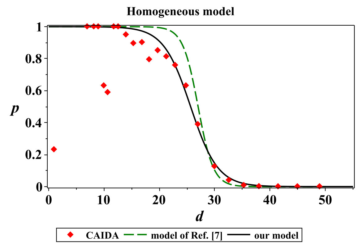 Figure 2
 Figure 4
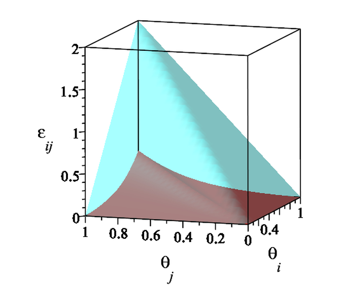 Figure 4
 Figure 5
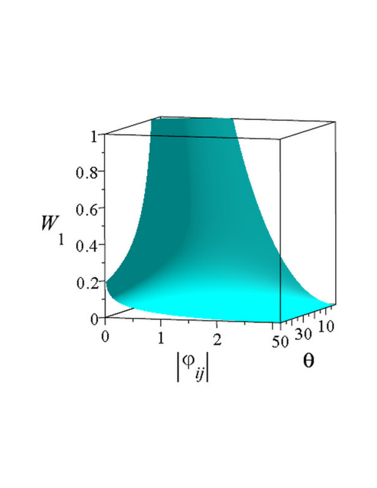 Figure 5
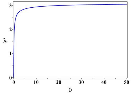 Figure 5
 Figure 6
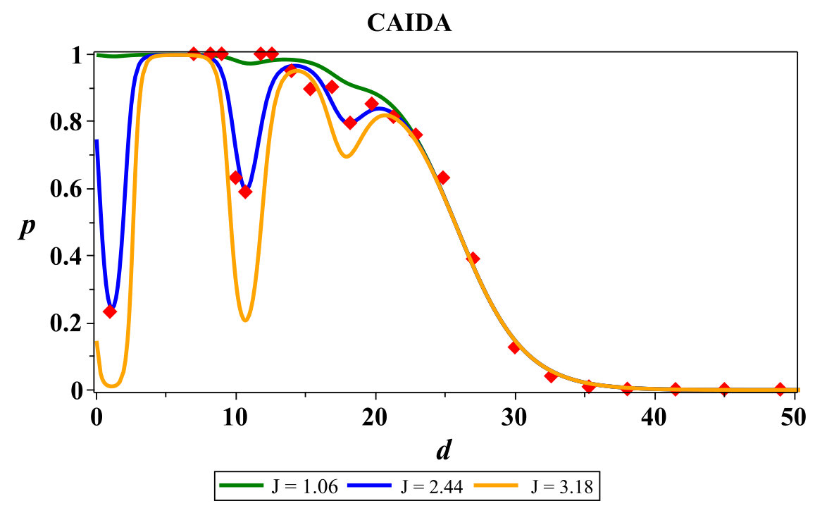 Figure 7
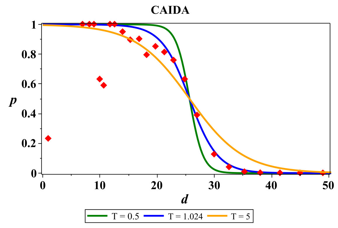 Figure 7
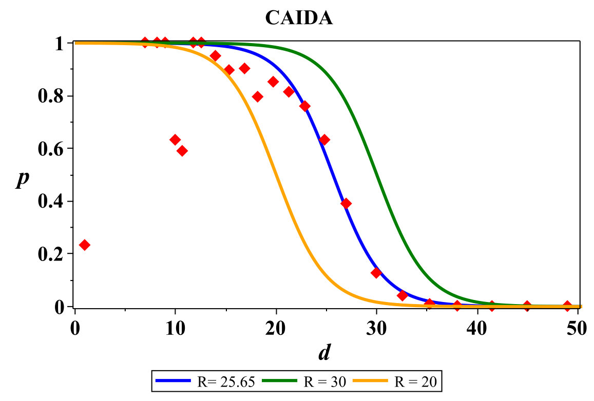 Figure 7
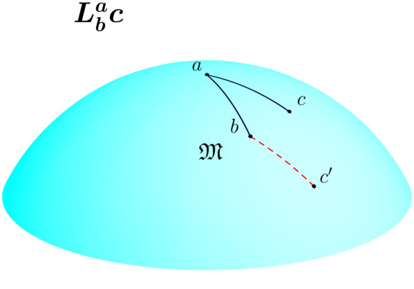 Figure 1
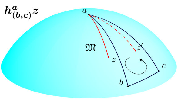 Figure 2
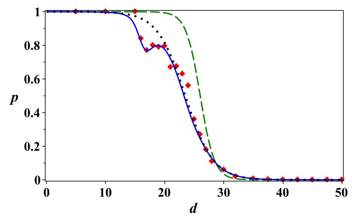 Figure 3
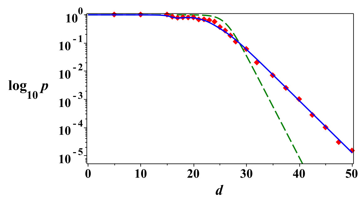 Figure 3
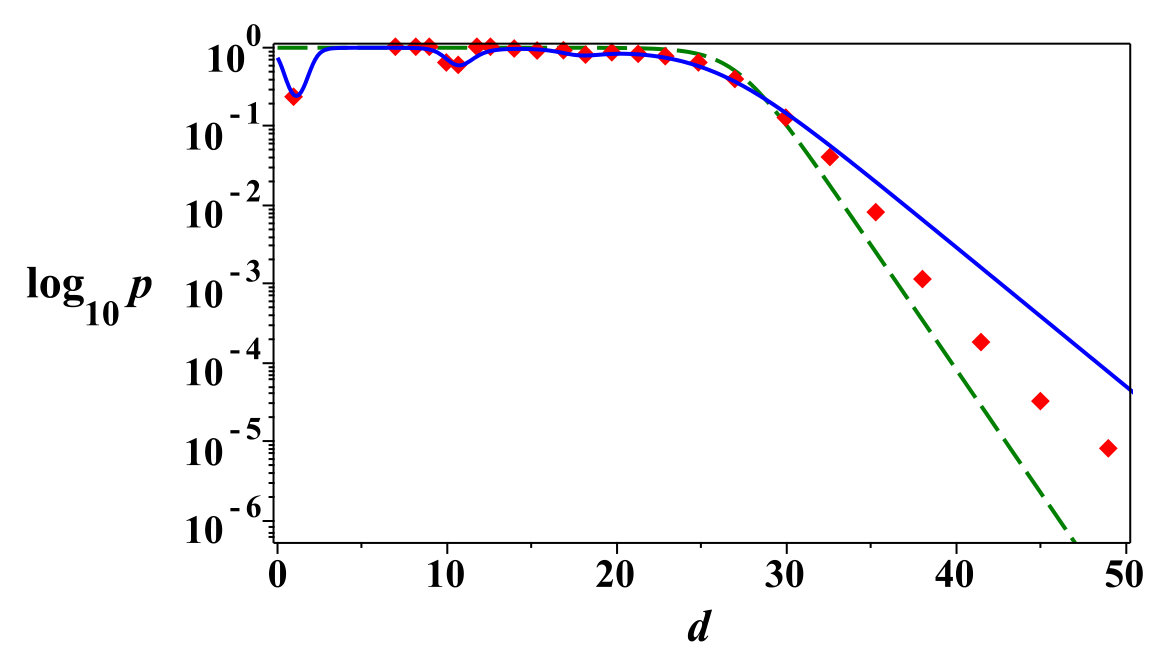 Figure 4
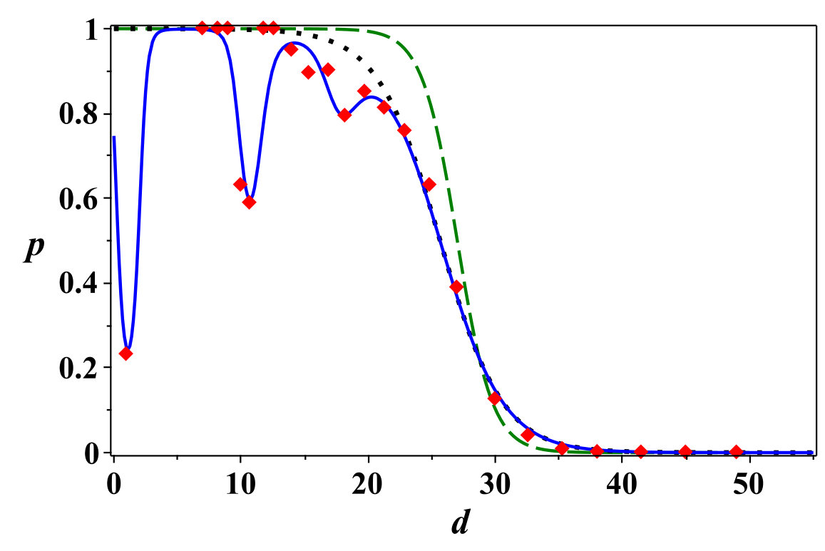 Figure 5
 Figure 8
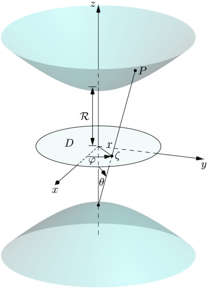 Figure 28
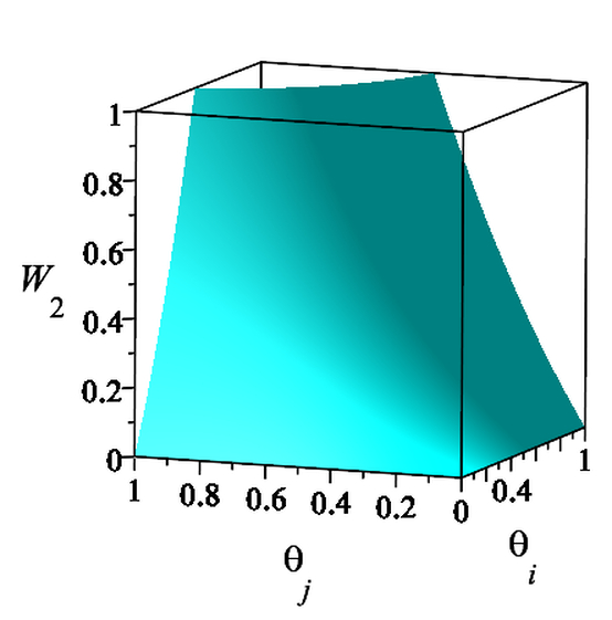 Figure 4
 Figure 4
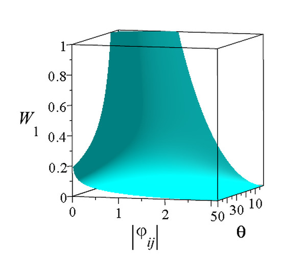 Figure 5
 Figure 5
Peer Reviews
No public reviews on file for this paper yet. If you reviewed it on a platform where reviews are public (OpenReview, ICLR, NeurIPS, ICML), you can paste yours below so the community can read it here.
Videos
No videos yet. Explain this paper in a talk, walkthrough, or lecture? Add one.
Complex Networks in the Framework of Nonassociative Geometry
Alexander I. Nesterov
Departamento de Física, CUCEI, Universidad de Guadalajara, Av. Revolución 1500, Guadalajara, CP 44420, Jalisco, México
Pablo Héctor Mata Villafuerte
Departamento de Física, CUCEI, Universidad de Guadalajara, Av. Revolución 1500, Guadalajara, CP 44420, Jalisco, México
Abstract
In the framework of on nonassociative geometry, we introduce a new effective model that extends the statistical treatment of complex networks with hidden geometry. The small-world property of the network is controlled by nonlocal curvature in our model. We use this approach to study the Internet as a complex network embedded in a hyperbolic space. The model yields a remarkable agreement with available empirical data and explains features of Internet connectance data that other models cannot. Our approach offers a new avenue for the study of a wide class of complex networks, such as air transport, social networks, biological networks, etc.
hyperbolic networks; complex networks; statistical mechanics; nonassociative geometry
pacs:
89.75.Hc, 89.20.Hh,02.50.-r, 05.30.-d
Due to its intrinsic interdisciplinary nature, Network Science can, and already has, contributed research in very diverse fields in both the natural sciences and the human world. Refinements in the techniques and methods of Network Science would therefore be of interest to a wide variety of researchers and, conceivably, policy makers and the general public.
Many real networks of large size, i.e. the Internet, the World Wide Web, airline networks, neural networks, citation networks, etc., are highly effective in exchanging information between distant nodes. This feature implies the existence of shortcuts between most pairs of nodes, and known as the small-world property Watts and Strogatz (1998); Boccaletti et al. (2006).
Complex Networks (CNs) have benefitted from the adoption of statistical mechanics as a powerful framework to explain properties of real-world networks Newman (2010); Newman et al. (2001); Newman (2003); Albert and Barabási (2002); Park and Newman (2004). The statistical physics approach has also been extended using geometric and topological ideas. Increasing attention to the geometrical and topological properties of CNs is focused on four main directions: characterization of the hyperbolicity of networks, emergence of network geometry, characterization of brain geometry, and network topology Bianconi (2015). In particular, in Krioukov et al. (2009, 2010); Boguñá et al. (2010) a duality between a highly heterogeneous degree distribution in a network and an underlying hyperbolic geometry was found and exploited for the realistic modeling of the Internet.
The exponential expansion of hyperbolic space illustrated in Fig.1 allows one to map an exponentially growing network to a hyperbolic space. In this context, the emergence of scaling in CNs can be explained by the hidden hyperbolic geometry Garlaschelli and Loffredo (2009); Serrano et al. (2008); Papadopoulos et al. (2012); A. et al. (2008); Verbeek and Suri (2016) (fundamental concepts concerning CNs, their statistical description and relation to hyperbolic geometry are treated in detail in Newman (2010); Newman et al. (2001); Albert and Barabási (2002); Krioukov et al. (2009, 2010); Park and Newman (2004); Garlaschelli and Loffredo (2009); A. et al. (2008); Boguñá et al. (2010); Boccaletti et al. (2006); Narayan and Saniee (2011); Bianconi and Rahmede (2017); Boguñá and Pastor-Satorras (2003); Bogacz et al. (2006); Bianconi (2015); Wang et al. (2016)).
The successful embedding of a CN in a geometric space invites the possibility of further exploiting the geometric properties of such CNs, namely by the known methods of differential geometry. The insights and calculational benefits of statistical mechanics could thus be complemented with those from geometry to form a more complete model. However, it is not obvious how the methods of differential geometry would apply to networks, which are fundamentally discrete structures. The main challenge is to define the curvature of networks. This is a hot mathematical topic, and different approaches to resolve it can be found in the literature Narayan and Saniee (2011); Bianconi (2015); Ollivier (2013); Sreejith et al. (2016); Saucan et al. (2019); Keller (2011); Estrada (2012); Estrada et al. (2014).
Nonassociative geometry Sabinin (1999); Nesterov and Sabinin (2000a, b), yielding an unified algebraic description of discrete spaces and smooth manifolds as well, opens a novel avenue for studying network geometry. The presence of curvature in a nonassociative space results in a non-trivial elementary holonomy, which is an equvialent of (nonlocal) curvature.
In this paper, we show how nonassociative geometry can be used to give a statistical description of CNs and reveal underlying geometry. We focus on the contribution from nonlocal curvature, described by elementary holonomy, to the statistical properties of CNs and find that nonlocal curvature controls the formation of a small-world network.
As a particular example, we perform a detailed study of the Internet embedded in a hyperboloic space. Our model shows excellent agreement with the empirical Internet connectance data. (All technical details concerning intermediate steps of our paper are presented in the Supplemental Material (SM).)
Nonassociative geometry in brief. – The main algebraic structures arising in nonassociative geometry are related to nonassociative algebra and the theory of quasigroups and loops (for details and review see Refs. Sabinin (1999, 1988, 1989, 1994); Nesterov and Mata (2019b)).
Consider a loop , i.e. a set with a binary operation (multiplication) , and the condition that each of the equations and has a unique solution: , . In addition, a two-sided identity holds: , where is a neutral element. A loop that is also a differential manifold with an operation that is a smooth map is called a smooth loop.
Nonassociativity of the operation is described by the identity , where is an associator. If , we obtain and, thus, a loop becomes a group. The multiplication of elements can also be written as , where is a left translation. In terms of left translations, the associator is given by .
The foundations of nonassociative geometry are based on the fact that in a neighborhood of an arbitrary point on a manifold with an affine connection one can introduce the geodesic local loop, which is uniquely defined by means of the parallel translation of geodesics along geodesics (Fig. 2).
The curvature of a nonassociative space is described by elementary holonomy, , where denotes a left translation with being a neutral element of the local loop. The elementary holonomy describes the parallel translation of the geodesic along the geodesic triangle (see Fig. 3). As one can see, it is some integral (nonlocal) curvature. If , we have a flat space.
As a particular example, we consider a nonassociative description of the two-dimensional hyperbolic space presented by the Poincaré disk model. Let be the open unit disk: . We define the nonassociative binary operation as
[TABLE]
where the bar denotes complex conjugation. The inverse operation is given by
[TABLE]
Inside , the set of complex numbers with the operation forms the two-sided loop QH(2) Nesterov (2000, 2001).
The associator on QH(2) is determined by
[TABLE]
Since the hyperboloid is a symmetric space, the elementary holonomy is determined by the associator: Sabinin (1988). The computation yields
[TABLE]
We define the left-invariant metric on as Nesterov and Mata (2019b)
[TABLE]
For a hyperbolic space with curvature the previous formula should be modified to read
[TABLE]
Taking , we find that
[TABLE]
For each triplet of points, , the elementary holonomy, , can be written as (see SM)
[TABLE]
where
[TABLE]
Supposing that , we obtain
[TABLE]
Here is the area of the geodesic triangle formed by the triplet of points .
The phase gained by an arbitrary “vector” during the parallel translation along the geodesic path , where denotes the geodesic connecting the points and , is given by
[TABLE]
This is consistent with the formula for the parallel transportation of a vector along a small contour (see SM):
[TABLE]
Here is the curvature tensor and is the area of the segment restricted by .
The loop QH(2) is isomorphic to the two-sheeted hyperboloid model (see SM for details). The isomorphism between the loop QH(2) and the upper sheet of the hyperboloid is established by , where are inner coordinates on . In the new variables, (7) yields the conventional metric on the hyperbolic space: .
To each pair of points one can assign the hyperbolic distance, , as follows Bianconi and Rahmede (2017):
[TABLE]
where and . The straightforward calculation shows that
[TABLE]
where , and for we obtain .
Complex networks in the framework of nonassociative geometry. – A network is a set of nodes (or vertices) connected by links (or edges). One can describe the network by an adjacency matrix, , where each existing or nonexisting link between pairs of nodes () is indicated by a 1 or 0 in the entry. Individual nodes possess local properties such as node degree (or connectivity) , and clustering coefficient Watts and Strogatz (1998); Boccaletti et al. (2006); Albert and Barabási (2002). The network as a whole can be described quantitatively by its degree distribution and connectance. The connectance is characterized by the connection probability , i.e. the probability that a pair nodes is connected.
The most general statistical description of an undirected network in equilibrium, with a fixed number of vertices and a varying number of links, is given by the grand canonical ensemble Park and Newman (2004); Garlaschelli et al. (2013); Garlaschelli et al. (2013). For a particular graph , the probability of obtaining this graph, , can be written as
[TABLE]
where is the graph Hamiltonian, denotes the partition function, and stands for inverse “temperature” of the network.
In what follows we restrict ourselves to consideration of a two-star model, one of the simplest and fundamental CN models. We assume that the CN is embedded in a hyperbolic space of constant curvature. The Hamiltonian describing the network generalizes the weighted two-star Hamiltonian introduced in Park and Newman (2004) and takes the form
[TABLE]
where is the weight of the edge , and are coupling constants, and denotes the elementary holonomy associated with the nodes . In our approach the weights are determined by the elementray holonomy and connectivity of the nodes.
The first term in (16) describes inhomogeneity in the distribution of links, resulting in natural clustering of nodes into cliques. Thus, one can expect that the holonomy (non-local curvature) is responsible for formation of the communities inside the CN Girvan and Newman (2002). To clarify this issue, let us rewrite (16) as , where the energy of the link is
[TABLE]
The first term in this expression describes the contribution to the energy to the link from the remaining nodes connected with the node by the shortest path. This leads to a mesoscopic inhomogeneity in the distribution of links, in a such way that nodes inside of the same group have very high degree, but between groups the connection is low.
The variables can be thought of as Ising pseudo-spins, , representing the edges connecting pairs of nodes in a network. We can thus map the network to the Ising model by setting , such that
[TABLE]
Inserting into Eq. (16), after some algebra we obtain
[TABLE]
where
[TABLE]
and we have used the notation h^{i}_{(jk)}=\frac{1}{2}\big{(}h^{i}_{jk}+h^{i}_{kj}\big{)}.
Within the mean field (MF) approximation, the Hamiltonian (21) is replaced by
[TABLE]
where denotes an expectation value, and the effective field, , is given by
[TABLE]
The total Hamiltonian of the system can be rewritten as , where is the Hamiltonian for a single pseudo-spin located on the edge , and
[TABLE]
Since the pseudo-spins in the MF approximation are decoupled, the partition function factorizes into a product of independent terms: . We obtain
[TABLE]
The computation of the expectation value for the pseudospin, , yields
[TABLE]
Inserting into Eq. (24), we obtain a self-consistent system of transcendental equations to determine the effective field,
[TABLE]
We are now in position to calculate the connectance of the network described by the connection probability, . Employing Eq. (27), we obtain
[TABLE]
The Internet as a complex hyperbolic network. – We turn now to the study of the Internet as a particular case of a scale-free CN embedded in a hyperbolic space , as considered in Krioukov et al. (2009, 2010); Boguñá et al. (2010). A scale-free network is characterized by a power-law degree distribution, , where is the node degree.
The Internet nodes are mapped to a hyperbolic space of curvature by assigning to each a random angular coordinate , and a radial coordinate () according to the radial node density
[TABLE]
where .
The size of the network is given by
[TABLE]
where is the average degree in the whole network and
[TABLE]
To adapt our model to empirical Internet data we consider as the independent variable in our calculations, thus allowing direct comparison to the results in Krioukov et al. (2009). We specify our model writing , where is the hyperbolic distance between nodes and . This yields the connection probability (29) in the form of the Fermi-Dirac distribution,
[TABLE]
where is the chemical potential, and
[TABLE]
The second term in this expression includes the contribution to the energy of the link from all nodes in the network and, thus, leads to the formation of “small world” communities Watts and Strogatz (1998).
Taking the distance between nodes as the independent variable, we find that the connection probability can be written as
[TABLE]
where
[TABLE]
and (for technical details see SM). When the coupling constant , our model simplifies to the model presented in Krioukov et al. (2009) and describes the homogeneous scale-free network with link energy .
In the framework of our model, the Internet temperature is defined from the following equation (for details see SM):
[TABLE]
where , is the average node degree of the CN, and denotes the Lerch transcendent Erdéley (1953). The chemical potential is given by
[TABLE]
[TABLE]
Table 1: Empirical Internet data and model parameters. BGP and CAIDA data are extracted from Refs. Krioukov et al. (2006); Boguñá et al. (2010).
As shown in the SM, at the point the system experiences a phase transition. Near the critical point, the chemical potential behaves as , and its derivative as . This agrees with conclusions made in Krioukov et al. (2010) on the behavior of the Internet size near the critical temperature.
Below the critical temperature the graph is completely disconnected, . In the limit of , we obtain
[TABLE]
We use Border Gateway Protocol (BGP) data and the Internet Archipelago data collected by the Cooperative Association for Internet Data Analysis (CAIDA), extracted from Refs. Krioukov et al. (2006); Boguñá et al. (2010), to estimate the size and temperature of the Internet embedded in the hyperbolic space, and the curvature of the space as well. Table 1 summarizes the empirical Internet data together with values of key model parameters.
Figs. 11 and 12 show the results of our numerical simulations and compare them with BGP data, CAIDA, and predictions by the model presented in Krioukov et al. (2009); Boguñá et al. (2010). We adapted the empirical connectance data for the BGP and CAIDA views of the Internet directly from Krioukov et al. (2009); Boguñá et al. (2010); Krioukov et al. (2006), and plotted them (red diamonds) along with the graph obtained from Eq.(102) (blue curves) and numerical results presented in Krioukov et al. (2009); Boguñá et al. (2010) (green dashed curves). (For details see Methods in SM.)
Our findings show that a homogeneous model () yields (in general) a good agreement with available empirical data (black dotted curve), but can not explain noticeable anomalies in the connection probability that break the scale-free behavior of the Internet. As one can see, the predictions of our complete (heterogeneous) model (blue curves) are in excellent agreement with the empirical data (red diamonds). The local minima in the connection probability around in the BGP case (Fig.11), and in the CAIDA case (Fig.12), are not artifacts in the empirical data but rather effect of small-world communities described by holonomy (nonlocal curvature).
Small world properties. – The small-world notion refers to the fact that for the most real networks the typical length, , defined as number of steps required to pass along the shortest path connecting two randomly chosen pair of nodes, could be relatively small Watts and Strogatz (1998).
We found that the homogeneous model reproduces all the small-world properties with remarkable accuracy. The contribution of the holonomy to the small-world geodesic distance is described by the corrections . Thus, one can say that the non-local curvature (described by the elementary holonomy) is responsible for formation of the ultra-small world effect Cohen and Havlin (2003); Chung and Lu (2002). However, the corrections are tiny and this point requires more thorough study to support our conjecture (For the technical details see SM.).
Communities formation. – The most real networks, including the Internet, exhibit inhomogeneity in the link distribution leading to the natural clustering of the network into groups or communities. Within the same community vertex-vertex connections are dense, but between groups connections are less dense Girvan and Newman (2002).
We found that for BGP and CAIDA experimental data, the holonomy exclusive model yields high level of the connection between nodes, (see SM for details). However, in the complete model we have . This means that there are many vertices with low degree and a small number with high degree. Our findings show that the holonomy is responsible for formation of the community structure of the Internet.
Concluding remarks.– Inspired by theoretical studies of networked systems that employ the methods of statistical physics and geometry, we introduced a general, flexible, and viable model for CNs with hidden geometry. Our approach incorporates the effects of nonlocal curvature and extends the statistical treatment of CNs. While we have considered CNs with hidden hyperbolic geometry, our model can be applied to the study of CNs with hidden geometry of space with arbitrary curvature as well.
We studied the Internet as a CN embedded in a hyperbolic space to explain features of Internet connectance data not only unexplained in previous studies, but completely unmentioned. We found an impressive agreement with available empirical data. To our best knowledge, this is the first model that explains all features of the Internet connectance data.
We show that non-local curvature is responsible for the formation of communities and ultra-small world network effects inside of the Internet. However, the corrections are tiny and our conjecture on the ultra-small world network formation requires more thorough study. This point will be addressed in future work.
Acknowledgements.
The authors acknowledge the support by the CONACYT.
Supplemental Material
Appendix A Poincaré disk model
The Poincaré disk model is related to the two-dimensional hyperbolic model as follows. Consider the two-sheeted hyperboloid, , defined in Cartesian coordinates by the equation: , the curvature of the hyperboloid being . We introduce the inner coordinates on the upper sheet of as follows:
[TABLE]
where the radial coordinate is and . Taking a point on the upper sheet of the hyperboloid, we project it to the plane by using the conversion formulas
[TABLE]
The nonassociative binary operation
[TABLE]
where the bar denotes complex conjugation, is defined for the neutral element located at the origin of coordinates. If the neutral element is chosen at the point , the operation (45) is modified as follows:
[TABLE]
where
[TABLE]
The computation of the associator and elementary holonomy yields
[TABLE]
In general, for any three vertices , , and , the elementary holonomy with respect to can be written as
[TABLE]
where
[TABLE]
and we set , .
For each triplet of nodes, , the elementary holonomy, , can be used as a measure of nonlocal curvature around . Indeed, for an arbitrary “vector”, , we obtain
[TABLE]
The phase gained by is found to be
[TABLE]
If we assume that , then we obtain
[TABLE]
Here is the area of the geodesic triangle formed by the triplet of points . Employing Eqs. (52) and (54), we obtain
[TABLE]
This is consistent with the formula for the parallel transport of the vector along a small contour :
[TABLE]
where is the curvature tensor and is the area of the segment enclosed by . Indeed, for a space of constant curvature , we have . For we obtain
[TABLE]
Appendix B Temperature of complex networks
The most general statistical description of an undirected network in equilibrium, with a fixed number of vertices and a varying number of links is given by the grand canonical ensemble Park and Newman (2004); Garlaschelli et al. (2013); Garlaschelli et al. (2013). For a graph model with energy given by , the connection probability between nodes and (i.e., the probability that the link exists), has the usual form of the Fermi-Dirac distribution:
[TABLE]
where is the energy of the link , and is the chemical potential. The chemical potential controls the link density and the connection probability, while the temperature, , controls clustering in the network. Below we will focus on a particular case, related to scale-free networks, where the link energy has a simple form: and .
Let us assign to each node a “hidden variable” . Then one can write the connection probability as
[TABLE]
where and . Suppose that is distributed as , where and Garlaschelli et al. (2013). This yields the distribution of according to .
We denote by the connection probability between two nodes with the fixed energy ,
[TABLE]
where denotes the set of all pairs having the energy , and is the total number of links (edges) belonging to . Replacing the sum by an integral, we obtain
[TABLE]
where
[TABLE]
The constant is defined by the normalization condition: . The computation yields
[TABLE]
To find the average node degree for the whole network, , we use the relationship , where is the number of total existing links,
[TABLE]
Assuming , we obtain
[TABLE]
Performing the integration, we find
[TABLE]
where and is the Lerch transcendent Erdéley (1953).
Let us consider a particular model with the chemical potential defined as , where is an unknown, temperature-independent parameter. Substituting in Eq.(66) and assuming , we obtain
[TABLE]
We further assume that and while . Then from Eq. (67) it follows that .
At the point the system experiences a phase transition. Below the critical temperature, , the graph is completely disconnected, . Near the critical point, for , the chemical potential behaves as and . In the limit of , we obtain and
[TABLE]
In summary, the average node degree is given by , where
[TABLE]
Comment. Since the temperature, , is an undetermined parameter, one can take the value of the critical temperature to be without loss of generality. If we have empirical information about the energy of the nodes and chemical potential, then we can define the temperature for a given network employing Eq.(65) (or Eq. (66)).
Appendix C Approximation of the connection probability
In what follows we consider a network with a large number of nodes, . First, we would like to calculate the connection probability between any two nodes and taking elementary holonomy into account. We can already state the form of as
[TABLE]
where is an inverse “temperature”. The effective field satisfies equation (24) of the main paper, which can be rewritten as follows:
[TABLE]
where and h^{i}_{(jk)}=({1}/{2})\big{(}h^{i}_{jk}+h^{i}_{kj}\big{)}. Computation of yields
[TABLE]
where . Using the identity
[TABLE]
one can show that
[TABLE]
Our important assumption, essential for further estimations, is that nodes are densely and uniformly distributed in their angular coordinates. This implies that the effective field depends only on the “radial” coordinates: . Then we can replace the sum over in (73) by an integral in the angular coordinate to get, after some algebra,
[TABLE]
where , and is the number of nodes located at the distance from the origin of coordinates. Further, it is convenient to rewrite (75) as
[TABLE]
To proceed further we use the anzatz , where
[TABLE]
and is a perturbation of the effective field. Employing Eq.(71), in the linear approximation we obtain
[TABLE]
Writing the connection probability as , where
[TABLE]
we find that
[TABLE]
When one can neglect the perturbation and use Eq.(79) instead of the exact expression given by Eq.(70). The computation of this quotient yields
[TABLE]
When over a large range of variables and , we can neglect the contributions from and use Eq. (77) for calculation of the effective field in .
Appendix D The Internet embedded in hyperbolic space
To adapt our model to empirical Internet data, such as BGP and CAIDA, we consider as the independent variable in our calculations, thus allowing direct comparison to the results in Krioukov et al. (2009) (the authors there use for distance rather than ). We average the connection probability over all pairs of nodes with fixed distance between them, writing
[TABLE]
where denotes the set of all pairs with distance between them, and is the total number of links (edges) in .
We write the effective field as , where
[TABLE]
and is given by (77). Substituting in Eq. (82), we find that , where
[TABLE]
and
[TABLE]
The approximate formula for the connection probability (84) will be valid when . This validity is discussed below in Sec. A. Further, we assume that is a homogeneous field, and we set . Using Eq. (77), we find
[TABLE]
Now substituting into Eq. (83), we obtain
[TABLE]
where
[TABLE]
What we now need is a practical way of evaluating this sum. We begin with the hyperbolic distance between a pair of nodes , as defined by Eq. (13) from the main paper:
[TABLE]
where . To find the dependence of the effective field on this distance we use Eq.(89), treating it as a constraint, , which allows us to eliminate either one of the variables or from consideration.
One can recast (89) in an equivalent form, writing
[TABLE]
where . When , we obtain
[TABLE]
Thus, one can approximate the distance as (i.e., the sum of the radial coordinates) if, for some threshold value , , where
[TABLE]
The graph of the function is depicted in Fig. 7 (left panel). For a given , the approximation is valid for , where (see Fig. 7, right panel). These figures show how the approximation works best at large distances between nodes, and is also valid for nearly any angle between them.
Now, we rewrite Eq. (89) as
[TABLE]
First, consider the case when and . Then the distance between nodes can be approximated as , if , where
[TABLE]
In the opposite case, when and , we obtain . For a given , this approximation is valid for , where
[TABLE]
(see Fig. 8, right panel). Next, for , we approximate the distance as , where is given by
[TABLE]
In Fig. 9 the function is depicted for (cyan surface) and (red surface).
Finally, according to the above analysis, the sum (88) can be approximated as the sum of three general cases which we can calculate approximately:
[TABLE]
where is the number of pairs in the interval , is the number of pairs inside the interval (or ) and , respectively. Applying the mean value theorem, we obtain
[TABLE]
where (), and as one can see . The unknown parameters, , determine the reference points in the application of the mean value theorem. Taking into account that and setting , we obtain
[TABLE]
Thus, we find that the connection probability is given by
[TABLE]
where
[TABLE]
and . The fitting parameters and should be fixed by comparing with available empirical data.
The connection probability (100) can be rewritten in the form of the Fermi-Dirac distribution:
[TABLE]
where is the chemical potential, and
[TABLE]
D.1 Validity of approximation
The approximation (100) is valid when . The computation yields
[TABLE]
where
[TABLE]
and
[TABLE]
Here is taken from Eq. (78). Next, using the relation
[TABLE]
one can recast Eq. (106) as
[TABLE]
where
[TABLE]
Replacing the sum by an integral, we we have
[TABLE]
where
[TABLE]
Once again applying the mean value theorem, we obtain
[TABLE]
Fig. 10 depicts the function . The choice of parameters corresponds to Figs. 4 and 5 of the main text. As one can see, the approximation is valid for a wide range of distances, and one can safely use Eq.(100) for computation of the connection probability.
Appendix E Methods
Parameters in our model are: temperature , size of the network , curvature , coupling constant ; fitting parameters and (). Taking into account that , we obtain nine independent parameters. These parameters should then be adjusted to make the model fit the available Internet data and, as we will see in the next section, can be reduced to six parameters if we have empirical values for , , and .
In our work, we use the empirical connectance data for the BGP and CAIDA views of the Internet, and map these data onto hyperbolic geometry, as described in Krioukov et al. (2006, 2009); Boguñá et al. (2010) (see Fig. 11).
Size and temperature of the Internet embedded in hyperbolic space
The Internet nodes are mapped to a hyperbolic space of curvature by assigning to each node a random angular coordinate , and a radial coordinate according to the radial node density:
[TABLE]
where and . As was shown above, the connection probability is given by the Fermi-Dirac distribution:
[TABLE]
where and
[TABLE]
When the coupling constant , the model describes the homogeneous scale-free network with the link energy .
The key formulae for embedding the Internet in the hyperbolic space are: the power-law degree distribution in the network, , and the expression for the average degree in the whole network, . In our model the control parameter is , and the size of the network is given by
[TABLE]
To determine we use the expression obtained in Krioukov et al. (2010); Garlaschelli et al. (2013) for the Internet embedded in the (universal) hyperbolic space with curvature ,
[TABLE]
The curvature, , of the target hyperbolic space is determined now by comparing (126) with (118). We obtain
[TABLE]
Internet temperature
Homogeneous model. – To estimate the Internet temperature, first we consider a purely homogeneous network (). Since the Internet is a scale-free sparse network, one can use Eq.(66) for the average node degree to determine the temperature of the Internet
[TABLE]
where the chemical potential is given by
[TABLE]
Substituting in (120), one can rewrite it as . For given and , solution of this equation yields .
Heterogeneous model. – In our complete model the coupling constant . Then, employing Eq. (65), we obtain
[TABLE]
where and are given by Eqs. (114) and (116), respectively. We use this expression to calculate the temperature of the Internet for the heterogeneous model.
In Table 1 we present the results of our computation of the Internet temperature for BGP and CAIDA data. The empirical data are extracted from Refs. Krioukov et al. (2009); Boguñá et al. (2010). As one can see, temperatures are very close for both models (homogeneous and heterogeneous).
[TABLE]
Table 1: The characteristics of the Internet: number of nodes (), number of links , average degree , exponent of degree distribution and temperature (). Empirical data are extracted from Refs. Krioukov et al. (2009); Boguñá et al. (2010)
*Impact of parameters. * – Fig. 12 presents our numerical results (black curve) and compares them with the theoretical predictions of the model presented in Krioukov et al. (2009); Boguñá et al. (2010) (green-dashed curve) and empirical Internet data obtained for BGP and CAIDA (red diamonds). Our findings show that a homogeneous model yields (in general) a good agreement with available empirical data, but can not explain evident anomalies in the connection probability that break the scale-free behavior of the Internet.
We found that parameters control the homogeneous, sigmoidal shape of the curve only, whereas the s and s regulate the location and depth of the local minima. Finally, the coupling constant controls the height of the local maxima.
In Fig. 13 we depict the connection probability for the homogeneous model with vanishing contribution from the holonomy () and compare the homogeneous model to the heterogeneous one for different values of paramaters and .
Community structure and small-world properties of the Internet
Community structure of the Internet. – Many real networks exhibit inhomogeneity in the link distribution, leading to the natural clustering of the network into groups or communities. Within the same community vertex-to-vertex connections are dense, but connections are less dense between groups Girvan and Newman (2002).
To study the contribution of holonomy to the formation of small communities, first we compare the connection probability for the exclusively holonomic model with the connection probability for homogeneous and heterogeneous models and empirical data (see Fig. 14). Additionally, we calculated the average node degree for the exclusively holonomic model. We found that for BGP and CAIDA experimental data, the model yields a high level of the connection between nodes, . This is close to the value of in the limit of high temperatures. However, in the complete model we have . This means that there are many vertices with low degrees and a small number with high degrees. Thus, our results show that holonomy (non-local curvature) is responsible for the formation of the community structure of the Internet:
*Small-world properties of the Internet. * – The small-world property of a network refers to a relatively short distance between randomly chosen pairs of nodes. In a small-world network the typical distance between nodes, , ( required to connect them by passing through other nodes) increases proportionally to the logarithm of the number of nodes, , as long as the clustering coefficient is not small Watts and Strogatz (1998). For a scale-free network with power-law degree distribution, and for , this dependence is modified as follows: the shortest path between two randomly chosen nodes grows as
[TABLE]
The presence of this behavior is known as the ultra small-world property of the scale-free network Cohen and Havlin (2003); Chung and Lu (2002).
To study small-world properties of the Internet embedded in hyperbolic space, we calculated the mean geodesic distance between two nodes for homogeneous () and heterogeneous models. The results are presented in Fig. 15. We found that for the homogeneous model. The contribution of the holonomy to the small-world effect is described by the corrections . Thus, one can say that the non-local curvature (described by the elementary holonomy) is responsible for formation of the ultra-small-world networks within the Internet. Since the corrections are tiny, support for our conjecture requires more thorough study.
To compare our findings with real networks we need to find the lowest number of steps required to pass from one node to other among pairs of nodes separated by the geodesic distance . If we let denote the mean geodesic distance per step, then the number of steps required to travel along the shortest path between a pair of nodes is given by . The main difficulty in the computation of is the lack of analytical results for free-scale networks. To overcome this obstacle, we note that for a high temperature the scale-free network becomes highly randomized, which allows us to employ the formula for the shortest distance in random networks given by Albert and Barabási (2002):
[TABLE]
In the limit of , every pair of nodes is connected with probability , and the computation of the average node degree yields . In the same limit we obtain and
[TABLE]
where
[TABLE]
Then the geodesic distance per step can be written as . Assuming that is a minimal geodesic distance per step (a “quant” of length), we obtain a qualitative formula for estimation of the path length,
[TABLE]
In Table 2 we compare our theoretical predictions with data available in the literature. We consider only the networks of large size, . As one can see, the predictions of Eq. (127) are in a reasonable qualitative agreement with the average path lengths of real networks.
[TABLE]
Table 2: The characteristics of some real networks: number of nodes (), average degree , average path length and temperature (). The columns , and show values of the average path lengths for random network (45), power-law degree distribution and our model (127), respectively.
The reference list from the paper itself. Each links out to its DOI / PubMed record.
- 1Watts and Strogatz (1998) D. J. Watts and S. H. Strogatz, “Collective dynamics of ‘small-world’ networks,” Nature 393 , 440 – 442 (1998).
- 2Boccaletti et al. (2006) S. Boccaletti, V. Latora, Y. Moreno, M. Chavez, and D.-U. Hwang, “Complex networks: Structure and dynamics,” Physics Reports 424 , 175 – 308 (2006) . · doi ↗
- 3Newman (2010) M. Newman, Networks: An Introduction (Oxford University Press, Inc., New York, NY, USA, 2010).
- 4Newman et al. (2001) M. E. J. Newman, S. H. Strogatz, and D. J. Watts, “Random graphs with arbitrary degree distributions and their applications,” Phys. Rev. E 64 , 026118 (2001).
- 5Newman (2003) M. E. J. Newman, “The structure and function of complex networks,” SIAM Review 45 , 167–256 (2003).
- 6Albert and Barabási (2002) R. Albert and A.-L. Barabási, “Statistical mechanics of complex networks,” Rev. Mod. Phys. 74 , 47–97 (2002).
- 7Park and Newman (2004) J. Park and M. E. J. Newman, “Statistical mechanics of networks,” Phys. Rev. E 70 , 066117 (2004).
- 8Bianconi (2015) G. Bianconi, “Interdisciplinary and physics challenges of network theory,” EPL 111 , 56001 (2015) .