Decomposition of Gaussian processes, and factorization of positive definite kernels
Palle Jorgensen, Feng Tian

TL;DR
This paper establishes a duality between factorizations of positive definite kernels and Gaussian processes, providing explicit correspondences and applications in various fields like point processes and graph Laplacians.
Contribution
It introduces a novel duality framework linking kernel factorizations with Gaussian process factorizations, addressing measure-theoretic challenges in infinite dimensions.
Findings
Explicit duality between kernel and Gaussian process factorizations
Measure-theoretic methods for infinite-dimensional factorizations
Applications to point processes, graph Laplacians, and boundary-value problems
Abstract
We establish a duality for two factorization questions, one for general positive definite (p.d) kernels , and the other for Gaussian processes, say . The latter notion, for Gaussian processes is stated via Ito-integration. Our approach to factorization for p.d. kernels is intuitively motivated by matrix factorizations, but in infinite dimensions, subtle measure theoretic issues must be addressed. Consider a given p.d. kernel , presented as a covariance kernel for a Gaussian process . We then give an explicit duality for these two seemingly different notions of factorization, for p.d. kernel , vs for Gaussian process . Our result is in the form of an explicit correspondence. It states that the analytic data which determine the variety of factorizations for is the exact same as that which yield factorizations for . Examples and applications are included:…
Click any figure to enlarge with its caption.
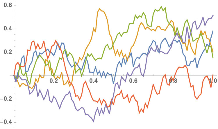 Figure 1
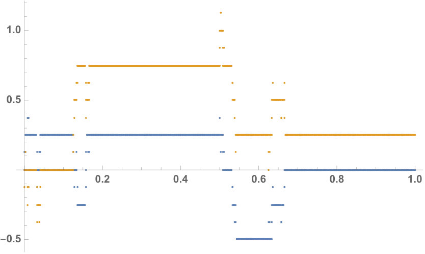 Figure 2
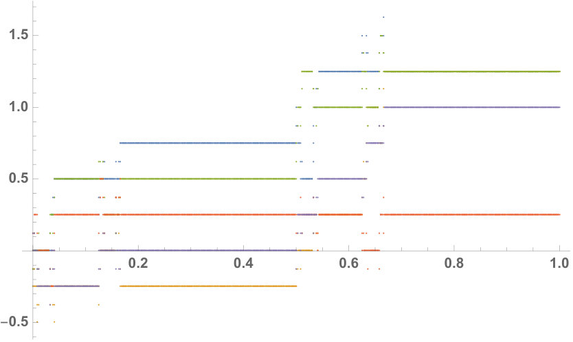 Figure 3
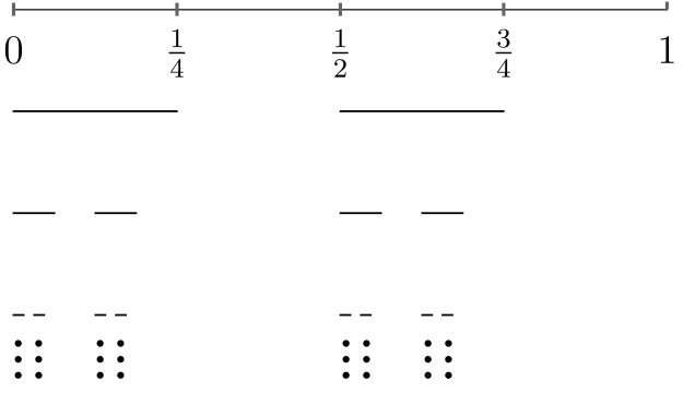 Figure 4
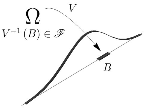 Figure 5
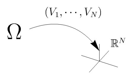 Figure 6
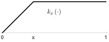 Figure 7
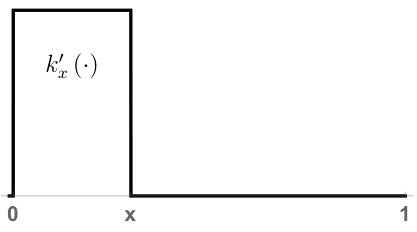 Figure 8
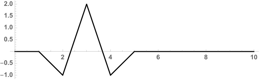 Figure 9
 Figure 10
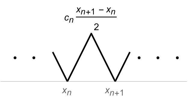 Figure 11
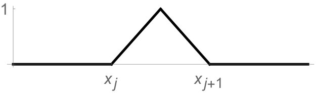 Figure 12
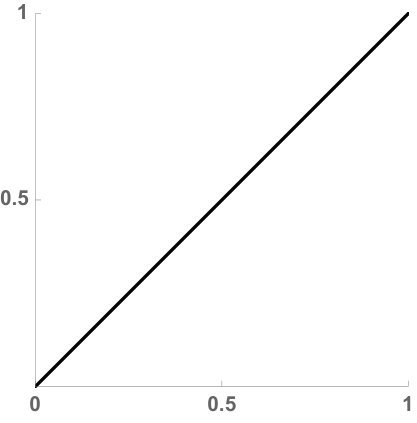 Figure 13
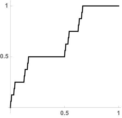 Figure 14
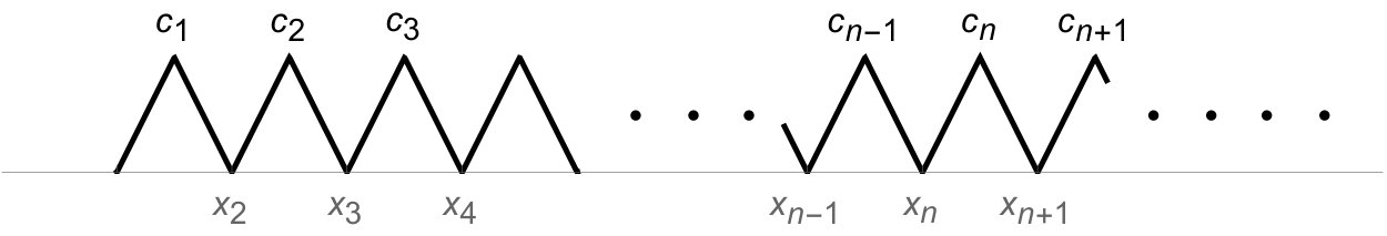 Figure 15
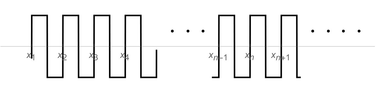 Figure 16
| , | ||||
| Ex 1 | ||||
| Ex 2 | on | |||
| Ex 3 | ||||
Peer Reviews
No public reviews on file for this paper yet. If you reviewed it on a platform where reviews are public (OpenReview, ICLR, NeurIPS, ICML), you can paste yours below so the community can read it here.
Videos
No videos yet. Explain this paper in a talk, walkthrough, or lecture? Add one.
Taxonomy
TopicsSpectral Theory in Mathematical Physics · Topological and Geometric Data Analysis · Matrix Theory and Algorithms
\RS@ifundefined
subsecref \newrefsubsecname = \RSsectxt
\RS@ifundefinedthmref \newrefthmname = theorem
\RS@ifundefinedlemref \newreflemname = lemma
\newreflemrefcmd=Lemma LABEL:#1 \newrefthmrefcmd=Theorem LABEL:#1 \newrefcorrefcmd=Corollary LABEL:#1 \newrefsecrefcmd=Section LABEL:#1 \newrefsubrefcmd=Section LABEL:#1 \newrefsubsecrefcmd=Section LABEL:#1 \newrefchaprefcmd=Chapter LABEL:#1 \newrefproprefcmd=Proposition LABEL:#1 \newrefexarefcmd=Example LABEL:#1 \newreftabrefcmd=Table LABEL:#1 \newrefremrefcmd=Remark LABEL:#1 \newrefdefrefcmd=Definition LABEL:#1 \newreffigrefcmd=Figure LABEL:#1
Decomposition of Gaussian processes, and factorization of positive
definite kernels
Palle Jorgensen
(Palle E.T. Jorgensen) Department of Mathematics, The University of Iowa, Iowa City, IA 52242-1419, U.S.A.
[email protected] http://www.math.uiowa.edu/~jorgen/ and
Feng Tian
(Feng Tian) Department of Mathematics, Hampton University, Hampton, VA 23668, U.S.A.
Abstract.
We establish a duality for two factorization questions, one for general positive definite (p.d) kernels , and the other for Gaussian processes, say . The latter notion, for Gaussian processes is stated via Ito-integration. Our approach to factorization for p.d. kernels is intuitively motivated by matrix factorizations, but in infinite dimensions, subtle measure theoretic issues must be addressed. Consider a given p.d. kernel , presented as a covariance kernel for a Gaussian process . We then give an explicit duality for these two seemingly different notions of factorization, for p.d. kernel , vs for Gaussian process . Our result is in the form of an explicit correspondence. It states that the analytic data which determine the variety of factorizations for is the exact same as that which yield factorizations for . Examples and applications are included: point-processes, sampling schemes, constructive discretization, graph-Laplacians, and boundary-value problems.
Key words and phrases:
Reproducing kernel Hilbert space, frames, generalized Ito-integration, the measurable category, analysis/synthesis, interpolation, Gaussian free fields, non-uniform sampling, optimization, transform, covariance, feature space.
2000 Mathematics Subject Classification:
Primary 47L60, 46N30, 46N50, 42C15, 65R10, 05C50, 05C75, 31C20, 60J20; Secondary 46N20, 22E70, 31A15, 58J65, 81S25, 68T05.
Contents
- 1 Introduction
- 2 Positive definite kernels
- 3 Gaussian processes
- 4 Sigma-finite measure spaces and Gaussian processes
- 5 Factorizations and stochastic integrals
- 6 Examples and applications
- 7 The case of when is atomic
- 8 Point processes: The case when
- 9 Boundary value problems
- 10 Sampling in
1. Introduction
We give an integrated approach to positive definite (p.d.) kernels and Gaussian processes, with an emphasis on factorizations, and their applications. Positive definite kernels serve as powerful tools in such diverse areas as Fourier analysis, probability theory, stochastic processes, boundary theory, potential theory, approximation theory, interpolation, signal/image analysis, operator theory, spectral theory, mathematical physics, representation theory, complex function-theory, moment problems, integral equations, numerical analysis, boundary-value problems for partial differential equations, machine learning, geometric embedding problems, and information theory. While there is no single book which covers all these applications, the reference [PR16] goes some of the way. As for the use of RKHS analysis in machine learning, we refer to [SZ07] and [Wes13].
Here, we give a new and explicit duality for positive definite functions (kernels) on the one hand, and Gaussian processes on the other. A covariance kernel for a general stochastic process is positive definite. In general, the stochastic process in question is not determined by its covariance kernel. But in the special case when the process is Gaussian, it is. In fact (3.1), every p.d. kernel is indeed the covariance kernel of a Gaussian process. The construction is natural; starting with the p.d. kernel , there is a canonical inductive limit construction leading to the Gaussian process for this problem, following a realization of Gaussian processes dating back to Kolmogorov. The interplay between analytic properties of p.d. kernels and their associated Gaussian processes is the focus of our present study.
We formulate two different factorization questions, one for general p.d. kernels , and the other for Gaussian processes, say . The latter notion, for Gaussian processes, is a subordination approach. Our approach to factorization for p.d. kernels is directly motivated by matrix factorizations, but in infinite dimensions, there are subtle measure theoretic issues involved. If the given p.d. kernel is already presented as a covariance kernel for a Gaussian process , we then give an explicit duality for these two seemingly different notions of factorization. Our main result, 5.1, states that the analytic data which determine the variety of factorizations for is the exact same as that which yield factorizations for .
2. Positive definite kernels
The notion of a positive definite (p.d.) kernel has come to serve as a versatile tool in a host of problems in pure and applied mathematics. The abstract notion of a p.d. kernel is in fact a generalization of that of a positive definite function, or a positive-definite matrix. Indeed, the matrix-point of view lends itself naturally to the particular factorization question which we shall address in 5 below. The general idea of p.d. kernels arose first in various special cases in the first half of 20th century: It occurs in work by J. Mercer in the context of solving integral operator equations; in the work of G. Szegő and S. Bergmann in the study of harmonic analysis and the theory of complex domains; and in the work by N. Aronszajn in boundary value problems for PDEs. It was Aronszajn who introduced the natural notion of reproducing kernel Hilbert space (RKHS) which will play a central role here; see especially (2.4) below. References covering the areas mentioned above include: [AJL17, Aro50, Hid80, IM65, Jor18, Jr68, JS18b], and [JT16c].
Right up to the present, p.d. kernels have arisen as powerful tools in many and diverse areas of mathematics. A partial list includes the areas listed above in the Introduction. An important new area of application of RKHS theory includes the following [ADD90, AD93, AB97, ADRdS01, ABK02, AM03, AD06, AL08].
Positive definite kernels and their reproducing kernel Hilbert spaces
Let be a set and let be a complex valued function on . We say that is positive definite (p.d.) iff (Def.) for all finite subset () and complex numbers , we have:
[TABLE]
In other words, the matrix is positive definite in the usual sense of linear algebra. We refer to the rich literature regarding theory and applications of p.d. functions [AJ12, JT16a, HKL*+*14, RAKK05, CXY15, Sko13, Her12].
We shall also need the Aronszajn [Aro50] reproducing kernel Hilbert spaces (R.K.H.S.), denoted : It is the Hilbert completion of all functions
[TABLE]
where , and , are as above.
If (finite) is fixed, and , are vectors in , we set
[TABLE]
With the definition of the R.K.H.S. , we get directly that the functions are automatically in ; and that, for all , we have
[TABLE]
i.e., the reproducing property holds.
Further recall (see e.g. [PR16]) that, given , then the R.K.H.S. is determined uniquely, up to isometric isomorphism in Hilbert space.
Lemma 2.1**.**
Let be a p.d. kernel, and let be the corresponding RKHS (see (2.3)-(2.4)). Let be a function defined on ; then TFAE:
- (i)
; 2. (ii)
there is a constant such that, for all finite subset , and all , , the following a priori estimate holds:
[TABLE]
Proof.
The implication (i)(ii) is immediate, and in this case, we may take .
Now for the converse, assume (ii) holds for some finite constant. On the -dense span in (2.2), define a linear functional
[TABLE]
From the assumption (2.5) in (ii), we conclude that (in (2.6)) is a well defined bounded linear functional on . Initially, is only defined on the span (2.2), but by (2.5), it is bounded, and so extends uniquely by -norm limits. We may therefore apply Riesz’ lemma to the Hilbert space , and conclude that there is a unique such that
[TABLE]
for all . Now, setting , for , we conclude from (2.7) that ; and so , proving (i). ∎
3. Gaussian processes
The interest in positive definite (p.d.) functions has at least three roots: (i) Fourier analysis, and harmonic analysis more generally; (ii) Optimization and approximation problems, involving for example spline approximations as envisioned by I. Schöenberg; and (iii) Stochastic processes. See [vNS41, Sch83].
Below, we sketch a few details regarding (iii). A stochastic process is an indexed family of random variables based on a fixed probability space. In some cases, the processes will be indexed by some group , or by a subset of . For example, , or , correspond to processes indexed by real time, respectively discrete time. A main tool in the analysis of stochastic processes is an associated covariance function.
A process is called Gaussian if each random variable is Gaussian, i.e., its distribution is Gaussian. For Gaussian processes, we only need two moments. So if we normalize, setting the mean equal to [math], then the process is determined by its covariance function. In general, the covariance function is a function on , or on a subset, but if the process is stationary, the covariance function will in fact be a p.d. function defined on , or a subset of . For a systematic study of positive definite functions on groups , on subsets of groups, and the variety of the extensions to p.d. functions on , see e.g. [JPT16].
By a theorem of Kolmogorov [Kol83], every Hilbert space may be realized as a (Gaussian) reproducing kernel Hilbert space (RKHS), see 3.1 below, and also [PS75, IM65, SNFBK10].
Now every positive definite kernel is also the covariance kernel of a Gaussian process; a fact which is a point of departure in our present analysis: Given a positive definite kernel, we shall explore its use in the analysis of the associated Gaussian process; and vice versa.
This point of view is especially fruitful when one is dealing with problems from stochastic analysis. Even restricting to stochastic analysis, we have the exciting area of applications to statistical learning theory [SZ07, Wes13].
Let be a probability space, i.e., is a fixed set (sample space), is a specified sigma-algebra (events) of subsets in , and is a probability measure on .
A Gaussian random variable is a function (in the real case), or , such that is measurable with respect to the sigma-algebra on , and the corresponding sigma-algebra of Borel subsets in (or in ). Let denote the expectation defined from , i.e.,
[TABLE]
The requirement on is that its distribution is Gaussian. If denotes a Gaussian on (or on ), the requirement is that
[TABLE]
or equivalently
[TABLE]
for all Borel sets ; see 3.1.
If , and are random variables, the Gaussian requirement is (see 3.2) that the joint distribution of is an -dimensional Gaussian, say , so if then
[TABLE]
For our present purpose we may restrict to the case where the mean (of the respective Gaussians) is assumed zero. In that case, a finite joint distribution is determined by its covariance matrix. In the case, it is specified as follows (the extension to is immediate) ,
[TABLE]
where denotes the standard Lebesgue measure on .
The following is known:
Theorem 3.1** (Kolmogorov [KR60], see also [Hid80, Hid92]).**
A kernel is positive definite if and only if there is a (mean zero) Gaussian process indexed by such that
[TABLE]
where denotes complex conjugation.
Moreover (see Hida [Hid71, Hid92]), the process in (3.6) is uniquely determined by the kernel in question. If is finite, then the covariance kernel for is given by
[TABLE]
for all , see (3.5) above.
In the subsequent sections, we shall address a number of properties of Gaussian processes important for their stochastic calculus. Our analysis deals with both the general case, and particular examples from applications. We begin in 4 with certain Wiener processes which are indexed by sigma-finite measures. For this class, the corresponding p.d. kernel has a special form; see (4.1) in 4.1. (The case of fractal measures is part of 6 below.) In 5, we address the general case: We prove our duality result for factorization, 5.1. The remaining sections are devoted to examples and applications.
4. Sigma-finite measure spaces and Gaussian processes
We shall consider functions of -finite measure space where is a set, a -algebra of subsets in , and is a positive measure defined on . It is further assumed that there is a countably indexed s.t. , ; and further that the measure space is complete; so the Radon-Nikodym theorem holds. We shall also restrict to the case when is assumed non-atomic. The case when is atomic is different, and is addressed in 7 below.
Definition 4.1**.**
Set
[TABLE]
Note then
[TABLE]
is positive definite. The corresponding Gaussian process is called the Wiener process [Hid71, Hid92]. In particular, we have
[TABLE]
and
[TABLE]
The precise limit in (4.3), quadratic variation, is as follows: Given as above, and , we then take limit over the filter of all partitions of (see (4.4)) relative to the standard notation of refinement:
[TABLE]
Details: Let , be the probability space which realizes as a Gaussian process (or generalized Wiener process), i.e., s.t. (4.2) holds for all pairs in . In particular, we have that , i.e., mean zero, Gaussian, and variance = . Then:
Lemma 4.2** (see e.g., [AJL17]).**
With the assumptions as above, we have
[TABLE]
where (in (4.5)) the limit is taken over the filter of all partitions of , and denotes the constant function “one” on .
As a result, we get the following Ito-integral
[TABLE]
defined for all , and
[TABLE]
We note that the following operator,
[TABLE]
is isometric.
In our subsequent considerations, we shall need the following precise formula (see 4.3) for the RKHS associated with the p.d. kernel
[TABLE]
defined on . We denote the RKHS by .
Lemma 4.3**.**
Let be as above, and let be the p.d. kernel on defined in (4.9). Then the corresponding RKHS is as follows: A function on is in if and only if there is a such that
[TABLE]
for all . Then
[TABLE]
Proof.
To show that in (4.10) is in , we must choose a finite constant such that, for all finite subset , , , , we get the following a priori estimate:
[TABLE]
But a direct application of Schwarz to shows that (4.12) holds, and for a finite , we may take , where is the -function in (4.10). The desired conclusion now follows from an application of 2.1.
We have proved one implication from the statement of the lemma: Functions on of the formula (4.10) are in the RKHS , and the norm is as stated in (4.11). In the below, we shall denote these elements in as pairs . We shall also restrict attention to the case of real valued functions.
For the converse implication, let be a function on , and assume . Then by Schwarz applied to we get
[TABLE]
where we used (4.11). Hence when Schwarz is applied to , we get a unique such that
[TABLE]
for all as in (4.10). Now specialize to , , in (4.14) and we conclude that
[TABLE]
which translates into the assertion that the pair has the desired form (4.10). And hence by (4.11) we have as stated. This concludes the proof of the converse inclusion. ∎
5. Factorizations and stochastic integrals
In Sections 2 and 3, we introduced the related notions of positive definite (p.d.) functions (kernels) on the one hand, and Gaussian processes on the other. One notes the immediate fact that a covariance kernel for a general stochastic process is positive definite. In general, the stochastic process in question is not determined by its covariance kernel. But in the special case when the process is Gaussian, it is.
In 3.1, we stated that every p.d. kernel is indeed the covariance kernel of a Gaussian process. The construction is natural; starting with the p.d. kernel , there is a canonical inductive limit construction leading to the Gaussian process for this problem. The basic idea for this particular construction of Gaussian processes dates back to pioneering work by Kolmogorov [Kol83, Hid80].
In the present section, we formulate two different factorization questions, one for general p.d. kernels , and the other for Gaussian processes, say . For details, see the respective definitions in (5.2) and (5.3) below. If is indeed the covariance kernel for a Gaussian process , it is natural to try to relate these two seemingly different notions of factorization. (In the case of Gaussian processes, a better name is perhaps “subordination” (see (5.10) below), but our theorem justifies the use of factorization in both of these contexts.) Our main result, 5.1, states that the data determining factorization for is the exact same as that which yields factorization for .
Let be a positive definite kernel ; and let be the corresponding Gaussian (mean zero) process, indexed by , i.e., , , and
[TABLE]
We set
[TABLE]
Further, if is the Gaussian process (from (5.1)), we set
[TABLE]
Following parallel terminology from measure theory, we say that a Gaussian process admits a disintegration, via suitable Ito-integrals, when there is a measure space with measure such that the corresponding Wiener process satisfies (5.3). Our theorem below (5.1) shows that this disintegration question may be decided instead by the answer to an equivalent spectral decomposition question; the latter of course formulated for the covariance kernel for . As is shown in the examples/applications below, given a Gaussian process, it is not at all clear what disintegrations hold; see for example 6.7.
Theorem 5.1**.**
Let be given positive definite, and let be the corresponding Gaussian (mean zero) process, then
[TABLE]
Proof.
We shall need the following: ∎
Lemma 5.2**.**
From the definition of , with fixed and assumed p.d., we get to every a natural isometry . It is denoted by
[TABLE]
and the adjoint operator is as follows: For all we have
[TABLE]
Moreover, we also have
[TABLE]
Proof.
Since , we have the factorization property (5.2), and so it follows from (5.5) that this extends by linearity and norm-completion to an isometry as stated.
By the definition of the adjoint operator , we have for :
[TABLE]
which is the assertion in the lemma.
From the properties of (see 2), it follows that (5.7) holds iff
[TABLE]
for all . But we may compute both sides in eq. (5.8) as follows:
[TABLE]
∎
Proof of 5.1 continued.
The proof is divided into two parts, one for each of the inclusions and in (5.4).
Part 1 “”. Assume a pair is in ; see (5.2). Then by definition, the factorization (5.3) holds on . Now let denote the Wiener process associated with , i.e., is a Gaussian process indexed by , and
[TABLE]
for all ; see (4.1) above. Now form the Ito-integral
[TABLE]
We stress that then , as defined by (5.10), is a Gaussian process indexed by . To see this, use the general theory of Ito-integration, see also [JS18b, JT17a, JT17b, JT16c, JT16b, Hid71, Hid80]. The approximation in (5.10) is over the filter of all *partitions *
[TABLE]
see (4.4). From the property of , , we conclude that, for all , we have that
[TABLE]
is Gaussian (mean zero) with
[TABLE]
where we used (5.11). Passing to the limit over the filter of all partitions of (as in (5.11)), we then get
[TABLE]
and with definition (5.10), therefore:
[TABLE]
where the last step in the derivation (5.14) uses the assumption that ; see (5.2).
Part 2 “”. Assume now that some pair is in where is given assumed p.d.; and where is “the” associated (mean zero) Gaussian process; i.e., with as its covariance kernel; see (5.1).
We claim that must then be in , i.e., that the factorization (5.3) holds. This in turn follows from the following chain of identities:
[TABLE]
valid for , and the conclusion follows. Note that the first step in the derivation of (5.15) uses the Ito-isometry. Hence, initially may possibly be the covariance kernel for a mean zero Gaussian process, say , different from . But we proved that the two Gaussian processes , and , have the same covariance kernel. It follows then the two processes must be equivalent. This is by general theory; see e.g. [Jr68, Itô04, AJL17].
The last uniqueness is only valid since we can consider Gaussian processes. Other stochastic processes are typically not determined uniquely from the respective covariance kernels. ∎
Remark 5.3*.*
In the statement of 5.1 there are two isometries: Starting with we get the canonical isometry given by
[TABLE]
see (5.5) of 5.2. But with , we then also get the Wiener process and the Ito-integral
[TABLE]
as an isometry. Here denotes the standard probability space, with abbreviation for the cylinder sigma-algebra of subsets of . For finite subsets in , and Borel subsets in , the corresponding cylinder set
[TABLE]
In summary, we get the the following diagram of isometries, corresponding to a fixed , where is a fixed p.d. function on :
6. Examples and applications
Below we present four examples in order to illustrate the technical points in 5.1. In the first example , the unit interval, and in the next two examples the open complex disk. In the fourth example, the Drury-Arveson kernel, we have .
We begin with a note on identifications: For , we set
[TABLE]
We write for the Lebesgue measure restricted to ; and we make the identification:
[TABLE]
Hence, for we have the familiar Fourier expansion: With
[TABLE]
[TABLE]
On , we shall also consider the Cantor measure with support equal to the Cantor set
[TABLE]
It is known that is the unique probability measure s.t.
[TABLE]
For the Fourier transform we have
[TABLE]
In 6.1, we summarize the three examples with the data from 5.1. We now turn to the details of the respective examples:
Example 6.1**.**
If is considered a kernel on , then the corresponding RKHS is the Hilbert space of functions on such that the distribution derivative is in , , , and
[TABLE]
and it is immediate that where , the indicator function; see 6.2.
The process is of course the standard Brownian motion on , pinned at ; see 6.3, and compare with the -process in 6.4. For Monte Carlo simulation, see e.g. [KBTB14, LCRK18].
The Hilbert space characterized by (6.6) is called the Cameron-Martin space, see e.g., [Hid80]. Moreover, to see that (6.6) is indeed the precise characterization of the RKHS for this kernel, one again applies 2.1.
It immediately follows from 5.1 then the Gaussian processes corresponding to the data in 6.1 are as follows:
Example 6.2**.**
:
[TABLE]
realized as an Ito-integral.
As an application of 5.1, we get:
[TABLE]
Example 6.3**.**
:
[TABLE]
were the -Ito integral is supported on the Cantor set , see 6.1.
As an application of 5.1, we get:
[TABLE]
The reasoning of 6.3 is based on a theorem of the paper [JP98] (see also [Jor18]). Set
[TABLE]
then the Fourier functions forms an orthonormal basis in , i.e., every has its Fourier expansion
[TABLE]
and
[TABLE]
Lemma 6.4**.**
Consider the set in (6.9), and, for , let
[TABLE]
be the corresponding generating function. Then we have the following infinite-product representation
[TABLE]
Proof.
From (6.9) we have the following self-similarity for : It is the following identity of sets
[TABLE]
Note that (6.12) is an algorithm for generating points in . Hence,
[TABLE]
and by induction.
Hence, if , the infinite-product is absolutely convergent, and the desired product formula (6.11) follows. ∎
Remark 6.5*.*
Note that, in combination with the theorem from [JP98] (see also [Jor18]), this property of the generating function from 6.4 is used in the derivation of the assertions made about the factorization properties in 6.3; this includes the two formulas (Ex 3) as stated in 6.1; as well as of the verification that , where , , and are as stated.
A direct computation of the two cases, 6.1 and 6.3, is of interest. Our result, 4.3, is useful in the construction: When computing the two Wiener processes and one notes that the covariance computed on intervals as are as follows:
[TABLE]
So the two functions have the representations as in 6.5.
Example 6.6**.**
The following example illustrates the need for a distinction between , and families of choices in 5.1. A priori, one might expect that if is given and p.d., it would be natural to try to equip with a -algebra of subsets, and a measure such that the condition in (5.2) holds for , i.e.,
[TABLE]
with a system in . It turns out that there are interesting examples where this is known to *not *be feasible. The best known such example is perhaps the Drury-Arveson kernel; see [Arv98] and [ARS08, ARS10].
Specifics. Consider for , and the complex ball defined for ,
[TABLE]
For , set
[TABLE]
Corollary 6.7** (Arveson [Arv98, Coroll 2]).**
Let , and let be the RKHS of the D-A kernel in (6.17). Then there is no Borel measure on such that ; i.e., there is no solution to the formula
[TABLE]
for all -polynomials.
Remark 6.8*.*
It is natural to ask about disintegration properties for the Gaussian process corresponding to the Drury-Arveson kernel (6.17). Combining our 5.1 above with the corollary (Coroll 6.7), we conclude that, in two or more complex dimensions , the question of finding the admissible disintegrations this Gaussian process is subtle. It must necessarily involve measure spaces going beyond .
7. The case of
when is atomic
Below we present a case where from pairs in may be chosen to be atomic. The construction is general, but for the sake of simplicity we shall assume that a given p.d. is such that the RKHS is separable, i.e., when it has an (all) orthonormal basis (ONB) indexed by .
Definition 7.1**.**
Let be a Hilbert space (separable), and let be a system of vectors in such that
[TABLE]
holds for all . We then say that is a Parseval frame for . (Also see 10.1.)
An equivalent assumption is that the mapping
[TABLE]
is isometric. One checks that then the adjoint is:
[TABLE]
For general background references on frames in Hilbert space, we refer to [HKLW07, KLZ09, SD13, KOPT13, HJL*+*13, Pes13, CM13, FPWW14, JT17b], and also see [KOPT13, Oko16, WO17, BBCO17, JS18a].
Lemma 7.2**.**
Let be given p.d. on , and assume that is a Parseval frame in ; then
[TABLE]
with the sum on the RHS in (7.3) absolutely convergent.
Proof.
By the reproducing property of , see 2, we get, for all :
[TABLE]
∎
Now a direct application of the argument in the proof of 5.1 yields the following:
Corollary 7.3**.**
Let be given p.d. on such that is separable, and let be a Parseval frame, for example an ONB in . Let be a chosen system of i.i.d. (independent identically distributed) system of standard Gaussians, i.e., with -distribution , . Then the following sum defines a Gaussian process,
[TABLE]
i.e., is well-defined in , as stated, where as a realization in an infinite Cartesian product with the usual cylinder -algebra, and has as covariance kernel, i.e.,
[TABLE]
see (5.15).
Proof.
This is a direct application of 7.2, and we leave the remaining verifications to the reader. ∎
8. Point processes: The case when
Let be a fixed positive definite kernel. We know that the RKHS consists of functions on subject to the a priori estimate in 2.1. For recent work on point-processes over infinite networks [JP19, JP14, JT18, JT16b, JT15b, GD18, QLS18, NP19, CH18], the case when the Dirac measures are in is of special significance. In this case there is an abstract Laplace operator , defined as follows:
[TABLE]
For the -norm of , we have
[TABLE]
immediate from (8.1).
For every finite subset , we consider the induced matrix
[TABLE]
Note that is a positive definite square matrix. Its spectrum consists of eigenvalues .
If is as described, i.e., p.d., and if
[TABLE]
we shall see that must then be discrete. (In interesting cases, also countable.) If (8.4) holds, we shall say that is a point process. We shall further show that point processes arise by restriction as follows:
Let be given with a p.d. kernel. If a countable subset is such that K^{\left(S\right)}:=K\big{|}_{S\times S} has
[TABLE]
then we shall say that is an induced point process.
8.1. Nets of finite submatrices, and their limits
Given as above with p.d. and defined on . Then the finite submatrices in the subsection header are indexed by the net of all finite subsets of as follows: Given , then the corresponding square matrix is simply the restriction of to . Of course, each matrix is positive definite, and so it has a finite list of eigenvalues. These eigenvalue lists figure in the discussion below.
Lemma 8.1**.**
Let , , and be as above, with denoting the numbers in the list of eigenvalues for the matrix . Then
[TABLE]
Proof.
Consider the eigenvalue equation
[TABLE]
From 2.1 and for , we then get
[TABLE]
Now apply to both sides in (8.8), and the desired conclusion (8.6) follows. ∎
Remark 8.2*.*
A consequence of the lemma is that the matrices and automatically are well defined (by the spectral theorem) with associated spectral bounds.
Definition 8.3**.**
Let , , and be as above; and with the condition in force. Set
[TABLE]
It is a finite-dimensional (and therefore closed) subspace in . The orthogonal projection onto will be denoted .
Lemma 8.4**.**
Let , , , and be as above. Then the orthogonal projection is as follows: For , set h_{F}=h\big{|}_{F}, restriction:
[TABLE]
Proof.
It is immediate from the definition that has the form
[TABLE]
with . Since is the orthogonal projection,
[TABLE]
(orthogonality in the -inner product) which yields:
[TABLE]
and therefore, , which is the desired formula (8.10). ∎
Corollary 8.5**.**
Let , , be as above, and assume for some . Then a function on is in if and only if
[TABLE]
where the supremum is over all finite subsets of . If is finite energy, then
[TABLE]
Proof.
The proof follows from an application of Hilbert space geometry to the RKHS , on the family of orthogonal projections indexed by the finite subsets in . With the standard lattice operations, applied to projections, we have . The conclusions (8.13)-(8.14) follow from this since, by the lemma,
[TABLE]
∎
Remark 8.6*.*
The advantage with the use of this system of orthogonal projections , indexed by the finite subsets of , is that we may then take advantage of the known lattice operations for orthogonal projections in Hilbert space. But it is important that we get approximation with respect to the canonical norm in the RKHS . This works because by our construction, the orthogonality properties for the projections refers precisely to the inner product in . Naturally we get the best -approximation properties when is further assumed countable. But the formula for the -norm holds in general.
Corollary 8.7**.**
Let be fixed, assumed p.d., and let be the corresponding RKHS. Let be given. Then if and only if
[TABLE]
In this case, we have:
[TABLE]
Proof.
The result is immediate from 8.5 applied to , where is fixed. Here the terms in (8.14) are, for finite, :
[TABLE]
and the stated conclusion is now immediate. ∎
Corollary 8.8**.**
Let , , and be as above, but assume now that is countable, with a monotone net of finite sets:
[TABLE]
then a function on is in iff \sup_{i}\left\|K_{F_{i}}^{-1/2}h\big{|}_{F_{i}}\right\|_{l^{2}\left(F_{i}\right)}<\infty.
Moreover,
[TABLE]
where, the convergence in (8.19) is monotone.
Proof.
From the definition of the order of orthogonal projections, we have
[TABLE]
and therefore,
[TABLE]
with . But by (8.15) and the proof of 8.5, we have
[TABLE]
and, so, by (8.21), we get:
[TABLE]
The conclusion now follows. ∎
8.2. Restrictions of p.d. kernels
Below we shall be considering pairs with a fixed p.d. kernel defined on , and, as before, we denote by the corresponding RKHS with its canonical inner product. In general, is an arbitrary set, typically of large cardinality, in particular uncountable: It may be a complex domain, a generalized boundary, or it may be a manifold arising from problems in physics, in signal processing, or in machine learning models. Moreover, for such general pairs , with a fixed p.d. kernel, the Dirac functions are typically not in .
Here we shall turn to induced systems, indexed by suitable countable discrete subsets of . Indeed, for a number of sampling or interpolation problems, it is possible to identify countable discrete subsets of , such that when is restricted to , i.e., K^{\left(S\right)}:=K\big{|}_{S\times S}, then for , the Dirac functions will be in ; i.e., we get induced point processes indexed by . In fact, with 8.8, we will be able to identify a variety of such subsets .
Moreover, each such choice of subset yields point-process, and an induced graph, and graph Laplacian; see (8.1)-(8.2). These issues will be taken up in detail in the two subsequent sections. In the following 8.9, for illustration, we identify a particular instance of this, when (the reals), and (the integers), and where is the covariance kernel of standard Brownian motion on .
Example 8.9** **(**Discretizing the covariance function for Brownian motion on
).**
The present example is a variant of 6.1, but with (instead of the interval ). We now set
[TABLE]
It is immediate that (6.6) in 6.1 carries over, but now with in place of . The normalization is carried over. We get that: A function on is in iff it has distribution-derivative in , see (8.23). As before, we conclude that the -norm is:
[TABLE]
see also 4.3.
Set
[TABLE]
and consider the corresponding RKHS . Using [JT15a, JT16a], we conclude that functions on are in iff , and
[TABLE]
In that case,
[TABLE]
For the -kernel, we have: , and
[TABLE]
Moreover, the corresponding Laplacian from (8.1) is
[TABLE]
i.e., the standard discretized Laplacian.
From the matrices , , we have the following; illustrated with .
[TABLE]
In particular, we have for :
[TABLE]
Remark 8.10*.*
The determinant of is 1 for all . Proof. By eliminating the first column, and then the first row, is reduced to . So by induction, the determinant is 1.
Note that
[TABLE]
which yields the factorization
[TABLE]
i.e.,
[TABLE]
where is the lower triangular matrix given by
[TABLE]
In particular, we get that immediately. This is a special case of 5.1.
For the general case, let be a finite subset of , assuming . Then the factorization (8.30) holds with
[TABLE]
Thus,
[TABLE]
In the setting of 5 (finite sums of standard Gaussians), we have the following: Let be as in (8.31), and let . Let be a system i.i.d. standard Gaussians , i.e., independent identically distributed. Set
[TABLE]
Then one checks that
[TABLE]
which is the desired Gaussian realization of .
Alternatively, assumes the following factorization via non-square matrices: Assume , then
[TABLE]
where is the matrix such that
[TABLE]
That is, takes the form:
[TABLE]
x_{1}$$x_{2}$$x_{3}$$x_{N}
Remark 8.11* (Spectrum of the matrices ; see also [HHT13]).*
It is known that the factorization as in (8.30) can be used to obtain the spectrum of positive definite matrices. The algorithm is as follows: Let be a given p.d. matrix.
Initialization: ;
Iterations: ,
- (i)
; 2. (ii)
;
Here in step (i) denotes the lower triangular matrix in the Cholesky decomposition of (see (8.30)). Then converges to a diagonal matrix consisting of the eigenvalues of .
We now resume consideration of the general case of p.d. kernels on and their restrictions: A setting for harmonic functions.
Remark 8.12*.*
In the general case of (8.2) and 8.1, we still have a Laplace operator . It is a densely defined symmetric operator on . Moreover (general case),
[TABLE]
(assuming that ). The dot “” in (8.37) refers to the action variable for the operator . In other words, is a generalized Greens kernel.
Definition 8.13**.**
Let be given p.d., and assume
[TABLE]
Let denote the induced Laplace operator. A function (in ) is said to be harmonic iff (Def.) .
Corollary 8.14**.**
Let be as above. Assume (8.38), and let be the induced Laplace operator. Then we have the following orthogonal decomposition for :
[TABLE]
where “clospan” in (8.39) refers to the norm in .
Proof.
It is immediate from (8.1) that
[TABLE]
where the orthogonality “” in (8.40) refers to the inner product . Since, by Hilbert space geometry, , we only need to observe that is closed in . But this is immediate from (8.1). ∎
Corollary 8.15** (Duality).**
Let be given, assumed p.d., and let be a countable subset such that
[TABLE]
- (i)
Then the following duality holds for the two induced kernels:
[TABLE]
both p.d. kernels on .
For every pair , we have the following matrix-inversion formula:
[TABLE]
where the summation on the LHS in (8.44) is a limit over a net of finite subsets , , s.t. ; and the result is independent of choice of net. 2. (ii)
We get an induced graph with as the set of vertices, and edge set as follows: .
An edge is a pair such that
[TABLE]
Proof.
The result follows from an application of Corollaries 8.7 and 8.8, and 8.12. ∎
Let , , and be as stated, countable infinite, with assumptions as in the previous two results. We showed that then the subset acquires the structure of a vertex set in an induced infinite graph (8.15 (ii)). If denotes the corresponding graph Laplacian, then the following boundary value problem is of great interest: Make precise the boundary conditions at “infinity” for this graph Laplacian . An answer to this will require identification of Hilbert space, and limit at “infinity.” The result below is such an answer, and the limit notion will be, limit over the filter of all finite subsets in ; see 8.7. Another key tool in the arguments below will again be the net of orthogonal projections from 8.4, and the convergence results from Corollaries 8.5 and 8.7.
Corollary 8.16**.**
Let , and be as in the statement of 8.15. Let denote the filter of finite subsets . Let be the graph Laplacian defined in (8.2), i.e.,
[TABLE]
for all , . Then the following equivalent conditions hold:
- (i)
For all ,
[TABLE] 2. (ii)
For , , ,
[TABLE] 3. (iii)
K_{F}\Delta P_{F}h=h\big{|}_{F}.
Proof.
On account of 8.8, we only need to verify (8.46). Let , , then we proved that
[TABLE]
Now apply to both sides in (8.47); and we get
[TABLE]
where we used . The desired conclusion (8.46) now follows from (8.49). Also note that if . ∎
8.3. Canonical isometries computed from point processes
Below we consider p.d. kernels defined initially on . Our present aim is to consider restrictions to when is a suitable subset of . Our first observation is the identification of a canonical isometry between the respective reproducing kernel Hilbert spaces; identifying as an isometric subspace inside . This isometry exists in general. However, we shall show that, when the subset is further restricted, the respective RKHSs, and isometry will admit explicit characterizations. For example, if is countable, and is the Dirac functions , , are in we shall show that this setting leads to a point process. In this case, we further identify an induced (infinite) graph with the set as vertices, and with associated edges defined by an induced kernel.
Theorem 8.17**.**
Let be a p.d. kernel, and let be a subset. Set K^{\left(S\right)}:=K\big{|}_{S\times S}. Let , and , be the respective RKHSs.
- (i)
Then there is a canonical isometric embedding
[TABLE]
given by the following formula: For , set
[TABLE]
(Note that on the LHS in (8.50) is a function on , while on the RHS is a function on .) 2. (ii)
The adjoint operator ,
[TABLE]
is given by restriction, i.e., if , and , then ; or equivalently, for all ,
[TABLE]
Proof.
To show that in (8.50) is isometric, proceed as follows: Let be a finite subset of , and , then
[TABLE]
which is the desired isometric property.
We now turn to (8.52), the restriction formula: Let , and , then
[TABLE]
But, for the LHS in (8.3), we have
[TABLE]
and so the desired formula (8.52) follows. ∎
Remark 8.18*.*
The canonical isometry for 8.9 (-discretization of the covariance function for Brownian motion on ). From 8.17, we know that the canonical isometry maps into ; see (8.22). But (8.23) and (8.25) in the Example offer exact characterization of these two Hilbert spaces. So, in the special case of 8.9, the canonical isometry maps from functions on into functions on . In view of (8.23), this assignment turns out to be a precise spline realization of the point grids realized by these sequences .
Below we present an explicit formula, and graphics, for the spline realizations. By (8.26), the embedding of from into is given by
[TABLE]
See 8.1. Therefore, for all , we get
[TABLE]
which is the spline interpolation.
Corollary 8.19**.**
Let be a p.d. kernel, and let be a subset. Assume further that . Then every finitely supported function on is in , and we have the following generalized spline interpolation; i.e., isometrically extending from to :
[TABLE]
where , and the sup is taken over the filter of all finite subsets of containing .
Proof.
Assume , supported on a finite subset . Then,
[TABLE]
where the last step follows from (8.10), and is the orthogonal projection from onto the subspace . ∎
Corollary 8.20**.**
Let , p.d.. be given, and let be a subset. Let , , be the canonical isometry. Then a function in satisfies if and only if
[TABLE]
Proof.
Immediate from part (ii) in 8.17. ∎
Remark 8.21*.*
Let be as in 8.20, and let be the canonical isometry. Let be the corresponding projection. Then is the projection onto the subspace given in (8.55).
Corollary 8.22**.**
Let be given p.d.; and let be a subset with induced kernel
[TABLE]
Consider the two sets and from (5.2) and 5.1. Let be the canonical isometry (8.50) in 8.17. Then the following implication holds:
[TABLE]
Proof.
Assuming (8.22), we get the representation (5.2):
[TABLE]
But then, for all , we then have
[TABLE]
which is the desired conclusion. ∎
9. Boundary value problems
Our setting in the present section is the discrete case, i.e., RKHSs of functions defined on a prescribed countable infinite discrete set . We are concerned with a characterization of those RKHSs which contain the Dirac masses for all points . Of the examples and applications where this question plays an important role, we emphasize two: (i) discrete Brownian motion-Hilbert spaces, i.e., discrete versions of the Cameron-Martin Hilbert space; (ii) energy-Hilbert spaces corresponding to graph-Laplacians.
The problems addressed here are motivated in part by applications to analysis on infinite weighted graphs, to stochastic processes, and to numerical analysis (discrete approximations), and to applications of RKHSs to machine learning. Readers are referred to the following papers, and the references cited there, for details regarding this: [AJS14, AJ12, AJL11, JPT15, JP14, JP11, DG13, Kre13, ZXZ09, Nas84, NS13].
The discrete case can be understood as restrictions of analogous PDE-models. In traditional numerical analysis, one builds discrete and algorithmic models (finite element methods), each aiming at finding approximate solutions to PDE-boundary value problems. They typically use multiresolution-subdivision schemes, applied to the continuous domain, subdividing into simpler discretized parts, called finite elements. And with variational methods, one then minimize various error-functions. In this paper, we turn the tables: our object of study are the discrete models, and analysis of suitable continuous PDE boundary problems serve as a tool for solutions in the discrete world.
Definition 9.1**.**
Let be a given p.d. kernel on . The RKHS is said to have the discrete mass property ( is called a discrete RKHS), if , for all .
In fact, it is known ([JT16a]) that every fundamental solution for a Dirichlet boundary value problem on a bounded open domain in , allows for discrete restrictions (i.e., vertices sampled in ), which have the desired “discrete mass” property.
We recall the following result to stress the distinction of the discrete models vs their continuous counterparts.
Let be a bounded, open, and connected domain in with smooth boundary . Let continuous, p.d., given as the Green’s function of , where
[TABLE]
for the Dirichlet boundary condition. Thus, is positive selfadjoint, and
[TABLE]
Let be the corresponding Cameron-Martin RKHS.
For , , take
[TABLE]
For , let
[TABLE]
Theorem 9.2**.**
Let , and , be given. Then
- (i)
Discrete case: Fix , , where , . Assume s.t. , , . Let
[TABLE]
then . 2. (ii)
Continuous case; by contrast: , but , .
Proof.
The result follows from an application of Corollaries 8.7 and 8.8. It extends earlier results [JT15a, JT16a] by the co-authors. ∎
10. Sampling in
In the present section, we study classes of reproducing kernels on general domains with the property that there are non-trivial restrictions to countable discrete sample subsets such that every function in has an -sample representation. In this general framework, we study properties of positive definite kernels with respect to sampling from “small” subsets, and applying to all functions in the associated Hilbert space .
We are motivated by concrete kernels which are used in a number of applications, for example, on one extreme, the Shannon kernel for band-limited functions, which admits many sampling realizations; and on the other, the covariance kernel of Brownian motion which has no non-trivial countable discrete sample subsets.
Definition 10.1**.**
Let be a p.d. kernel, and be the associated RKHS. We say that has non-trivial sampling property, if there exists a countable subset , and , such that
[TABLE]
If equality holds in (10.1) with , then we say that is a Parseval frame. (Also see 7.1.)
It follows that sampling holds in the form
[TABLE]
if and only if is a Parseval frame.
Lemma 10.2**.**
Suppose , , , , and satisfy the condition in (10.1), then the linear span of is dense in . Moreover, there is a positive operator in with bounded inverse such that
[TABLE]
is a convergent interpolation formula valid for all .
Equivalently,
[TABLE]
Proof.
Define by , . Then the adjoint operator is given by , , and
[TABLE]
holds in , with -norm convergence. Now set , and note that , where is in the lower bound in (10.1). ∎
Theorem 10.3**.**
Let be a p.d. kernel, and let be a countable discrete subset. For all , set . Then TFAE:
- (i)
The family is a Parseval frame in ; 2. (ii)
[TABLE] 3. (iii)
[TABLE] 4. (iv)
[TABLE]
where the sum converges in the norm of .
Proof.
The proof is simple, and follows the steps in the proof of 7.2. Details are left to the reader. ∎
We now turn to dichotomy: Existence of countably discrete sampling sets vs non-existence.
Example 10.4**.**
Let , and let be the Shannon kernel, where
[TABLE]
We may choose , and then is even an orthonormal basis (ONB) in , but there are many other examples of countable discrete subsets such that (10.1) holds for finite .
The RKHS in (10.2) is the Hilbert space consisting of all such that , where “suppt” stands for support of the Fourier transform . Note consists of functions on which have entire analytic extensions to . Using the above observations, we get
[TABLE]
Example 10.5**.**
Let be the covariant kernel of standard Brownian motion, with or , and
[TABLE]
Theorem 10.6**.**
Let , be as in (10.3); then there is no countable discrete subset such that is dense in .
Proof.
Suppose , where
[TABLE]
then consider the following function
[TABLE]
On the respective intervals , the function is as follows:
[TABLE]
In particular, , and on the midpoints:
[TABLE]
see 10.1.
Choose such that
[TABLE]
Admissible choices for the slope-values include
[TABLE]
We will now show that . For the distribution derivative computed from (10.5), we get
[TABLE]
[TABLE]
which is the desired conclusion, see (10.5). ∎
Corollary 10.7**.**
For the kernel in (10.3), , the following holds:
Given , , then the interpolation problem
[TABLE]
is solvable if
[TABLE]
Proof.
Let be the piecewise linear spline (see 10.2) for the problem (10.8), see 10.2; then the -norm is as follows:
[TABLE]
when (10.9) holds. ∎
Remark 10.8*.*
Let be as in (10.3), . For all , let
[TABLE]
Assuming (10.6) holds, then
[TABLE]
Theorem 10.9**.**
Let be a set of cardinality of the continuum, and let be a positive definite kernel. Let be a discrete subset of . Suppose there are weights , , such that
[TABLE]
for all . Suppose further that there is a point , a , and such that the infimum
[TABLE]
is strictly positive.
Then is not a interpolation set for .
Proof.
This results follows from 10.2 and 10.3 above. We also refer readers to [JT16b]. ∎
Acknowledgement*.*
The co-authors thank the following colleagues for helpful and enlightening discussions: Professors Daniel Alpay, Sergii Bezuglyi, Ilwoo Cho, Myung-Sin Song, Wayne Polyzou, and members in the Math Physics seminar at The University of Iowa.
The reference list from the paper itself. Each links out to its DOI / PubMed record.
- 1[AB 97] D. Alpay and V. Bolotnikov, On tangential interpolation in reproducing kernel Hilbert modules and applications , Topics in interpolation theory (Leipzig, 1994), Oper. Theory Adv. Appl., vol. 95, Birkhäuser, Basel, 1997, pp. 37–68. MR 1473250
- 2[ABK 02] Daniel Alpay, Vladimir Bolotnikov, and H. Turgay Kaptanoğlu, The Schur algorithm and reproducing kernel Hilbert spaces in the ball , Linear Algebra Appl. 342 (2002), 163–186. MR 1873434
- 3[AD 93] Daniel Alpay and Harry Dym, On a new class of structured reproducing kernel spaces , J. Funct. Anal. 111 (1993), no. 1, 1–28. MR 1200633
- 4[AD 06] D. Alpay and C. Dubi, Some remarks on the smoothing problem in a reproducing kernel Hilbert space , J. Anal. Appl. 4 (2006), no. 2, 119–132. MR 2223568
- 5[ADD 90] Daniel Alpay, Patrick Dewilde, and Harry Dym, Lossless inverse scattering and reproducing kernels for upper triangular operators , Extension and interpolation of linear operators and matrix functions, Oper. Theory Adv. Appl., vol. 47, Birkhäuser, Basel, 1990, pp. 61–135. MR 1120274
- 6[AD Rd S 01] D. Alpay, A. Dijksma, J. Rovnyak, and H. S. V. de Snoo, Realization and factorization in reproducing kernel Pontryagin spaces , Operator theory, system theory and related topics (Beer-Sheva/Rehovot, 1997), Oper. Theory Adv. Appl., vol. 123, Birkhäuser, Basel, 2001, pp. 43–65. MR 1821907
- 7[AJ 12] Daniel Alpay and Palle E. T. Jorgensen, Stochastic processes induced by singular operators , Numer. Funct. Anal. Optim. 33 (2012), no. 7-9, 708–735. MR 2966130
- 8[AJL 11] Daniel Alpay, Palle Jorgensen, and David Levanony, A class of Gaussian processes with fractional spectral measures , J. Funct. Anal. 261 (2011), no. 2, 507–541. MR 2793121