Semiparametric Difference-in-Differences with Potentially Many Control Variables
Neng-Chieh Chang

TL;DR
This paper introduces three new semiparametric difference-in-differences estimators that effectively handle many control variables, including high-dimensional cases, achieving bias reduction, sqrt{N}-consistency, and valid inference.
Contribution
It proposes novel DID estimators that incorporate machine learning methods for high-dimensional controls, overcoming bias and inconsistency issues of traditional approaches.
Findings
New estimators achieve sqrt{N}-consistency and asymptotic normality.
Estimators have the small bias property, with bias diminishing faster than nonparametric estimators.
Method enables valid inference with many control variables, including high-dimensional settings.
Abstract
This paper discusses difference-in-differences (DID) estimation when there exist many control variables, potentially more than the sample size. In this case, traditional estimation methods, which require a limited number of variables, do not work. One may consider using statistical or machine learning (ML) methods. However, by the well-known theory of inference of ML methods proposed in Chernozhukov et al. (2018), directly applying ML methods to the conventional semiparametric DID estimators will cause significant bias and make these DID estimators fail to be sqrt{N}-consistent. This article proposes three new DID estimators for three different data structures, which are able to shrink the bias and achieve sqrt{N}-consistency and asymptotic normality with mean zero when applying ML methods. This leads to straightforward inferential procedures. In addition, I show that these new…
Click any figure to enlarge with its caption.
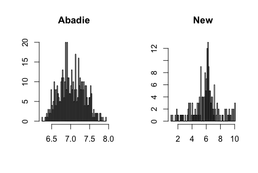 Figure 1
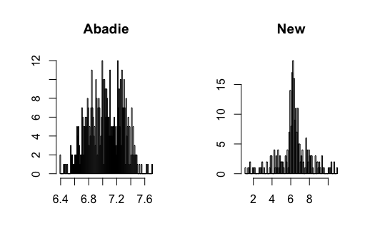 Figure 2
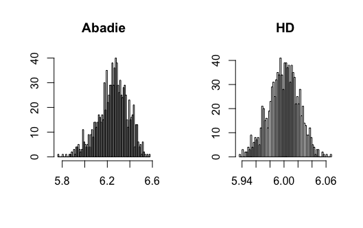 Figure 3
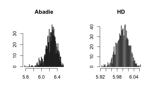 Figure 4
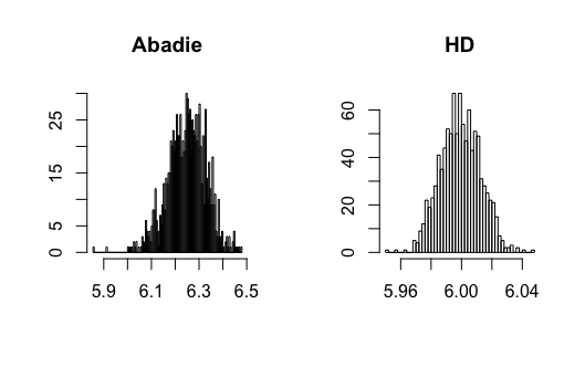 Figure 5
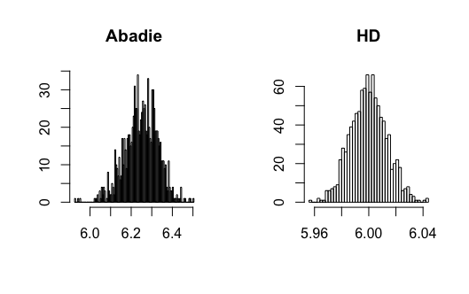 Figure 6
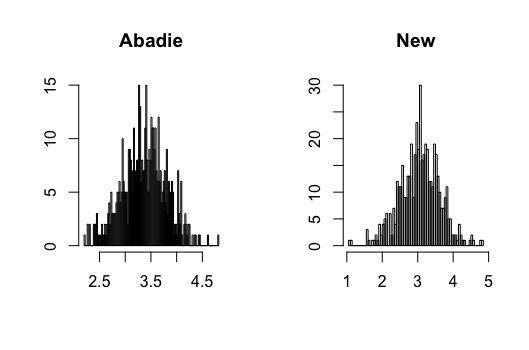 Figure 7
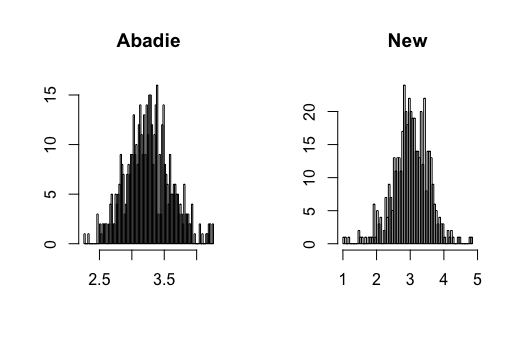 Figure 8
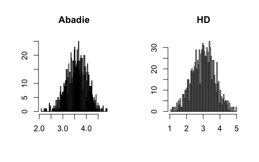 Figure 9
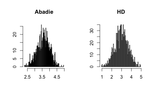 Figure 10
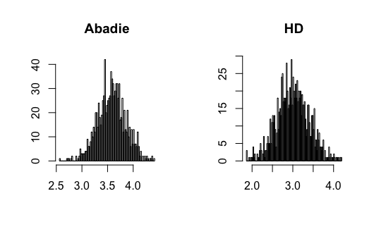 Figure 11
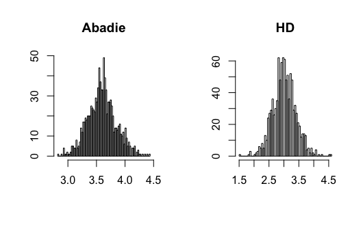 Figure 12
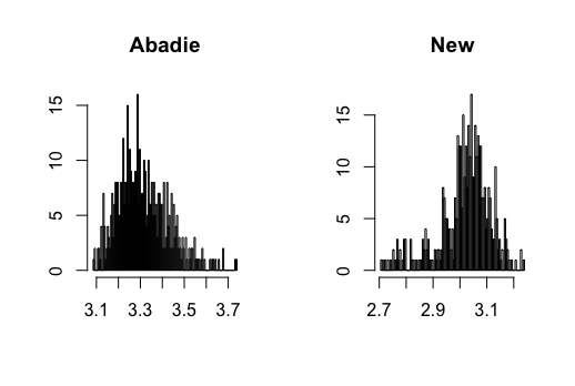 Figure 13
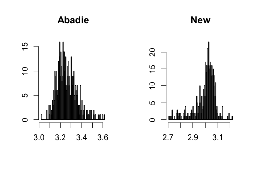 Figure 14
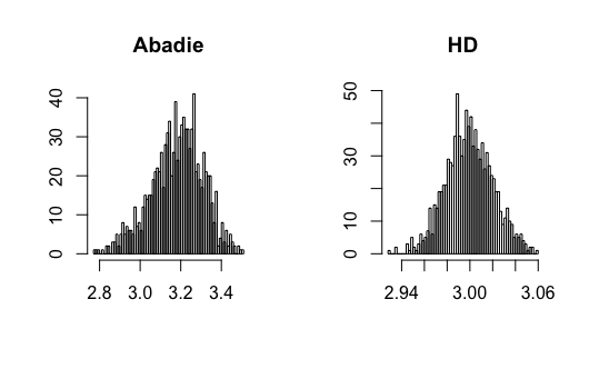 Figure 15
 Figure 16
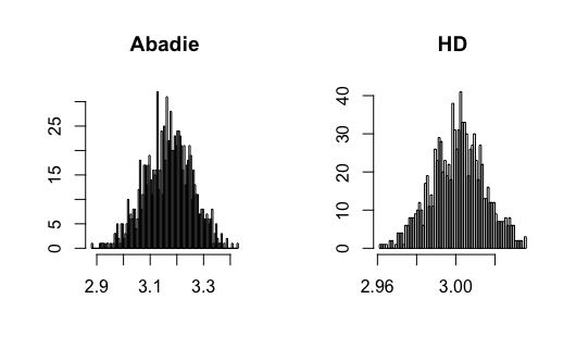 Figure 17
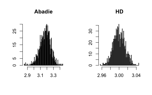 Figure 18
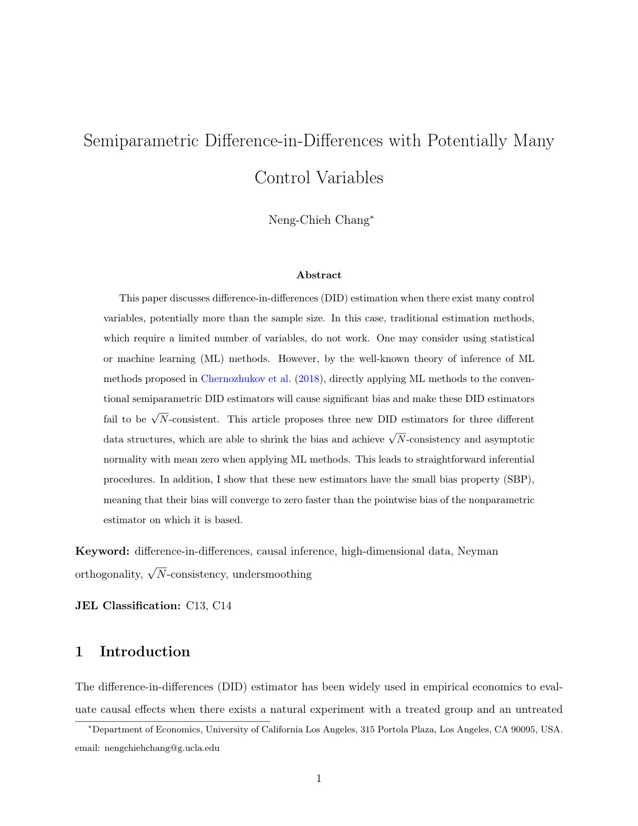 Figure 19
| Sequeira (2016) | Abadie (kernel) | (kernel) | Abadie (Lasso) | (Lasso) | |
|---|---|---|---|---|---|
| ATT | -2.928** (0.944) | -7.986** (3.028) | -8.670** (3.643) | -7.499** (2.746) | -9.191* (4.854) |
Peer Reviews
No public reviews on file for this paper yet. If you reviewed it on a platform where reviews are public (OpenReview, ICLR, NeurIPS, ICML), you can paste yours below so the community can read it here.
Videos
No videos yet. Explain this paper in a talk, walkthrough, or lecture? Add one.
Taxonomy
TopicsAdvanced Causal Inference Techniques
Semiparametric Difference-in-Differences with Potentially Many Control Variables
Neng-Chieh Chang111Department of Economics, University of California Los Angeles, 315 Portola Plaza, Los Angeles, CA 90095, USA. email: [email protected]
Abstract
This paper discusses difference-in-differences (DID) estimation when there exist many control variables, potentially more than the sample size. In this case, traditional estimation methods, which require a limited number of variables, do not work. One may consider using statistical or machine learning (ML) methods. However, by the well-known theory of inference of ML methods proposed in Chernozhukov \BOthers. (\APACyear2018), directly applying ML methods to the conventional semiparametric DID estimators will cause significant bias and make these DID estimators fail to be -consistent. This article proposes three new DID estimators for three different data structures, which are able to shrink the bias and achieve -consistency and asymptotic normality with mean zero when applying ML methods. This leads to straightforward inferential procedures. In addition, I show that these new estimators have the small bias property (SBP), meaning that their bias will converge to zero faster than the pointwise bias of the nonparametric estimator on which it is based.
Keyword: difference-in-differences, causal inference, high-dimensional data, Neyman orthogonality, -consistency, undersmoothing
JEL Classification: C13, C14
1 Introduction
The difference-in-differences (DID) estimator has been widely used in empirical economics to evaluate causal effects when there exists a natural experiment with a treated group and an untreated group. By comparing the variation over time in an outcome variable between the treated group and the untreated group, the DID estimator can be used to calculate the effect of treatment on the outcome variable. Applications of DID include but are not limited to studies of the effects of immigration on labor markets (Card, \APACyear1990), the effects of minimum wage law on wages (Card \BBA Krueger, \APACyear1994), the effect of tariffs liberalization on corruption (Sequeira, \APACyear2016), the effect of household income on children’s personalities (Akee, Copeland, Costello\BCBL \BBA Simeonova, \APACyear2018), and the effect of corporate tax on wages (Fuest, Peichl\BCBL \BBA Siegloch, \APACyear2018).
The traditional linear DID estimator depends on a parallel trend assumption that in the absence of treatment, the difference of outcomes between treated and untreated groups remains constant over time. In many situations, however, this assumption may not hold because there are other individual characteristics that may be associated with the variations of the outcomes. The treatment may be taken as exogenous only after controlling these characteristics. To address this problem, Abadie (\APACyear2005) proposed the semiparametric DID estimators. Compared to the traditional linear DID estimators, the advantages of Abadie’s estimators are threefold. First, the characteristics are treated nonparametrically so that any estimation error caused by functional specification is avoided. Second, the effect of treatment is allowed to vary among individuals, while the traditional linear DID estimator does not allow this heterogeneity. Third, the estimation framework proposed in Abadie (\APACyear2005) allows researchers to estimate how the effect of treatment varies with changes in the characteristics.
This paper is an extension of Abadie (\APACyear2005). Abadie (\APACyear2005) considered the case where the number of control variables has to be limited. A practical difficulty empirical researchers encounter is choosing what variables to include when there is a rich data set. Although economic intuition can help us narrow down the choice set, it will not completely select all the important variables. This variable selection problem may lead to the chance of omitted variables in practice. In this paper, I consider the DID estimation with many control variables, potentially more than the sample size. The classical estimation methods which require a fixed number of variables do not work in this situation. One has to consider using ML methods such as Lasso, Logit Lasso, random forests, boosted trees, or various hybrids. However, by the well-known theory of inference of ML methods developed in Chernozhukov \BOthers. (\APACyear2018), if one directly applies ML methods to the conventional semiparametric DID estimators proposed in Abadie (\APACyear2005), the result will lead to significant bias and invalid inference. In particular, the regularization bias embedded in ML methods will result in the conventional semiparametric DID estimators failing to be -consistent.
I contribute to the literature by proposing three new DID estimators for three different data structures: repeated outcomes, repeated cross-sections, and multilevel treatment. These new estimators can relieve the impact of the regularization bias of ML methods and achieve -consistency. The key is to find the so-called Neyman-orthogonal scores (Chernozhukov \BOthers., \APACyear2018) of Abadie (\APACyear2005)’s estimands. The Neyman-orthogonal score is a function that identifies the parameter of interest, and its derivatives with respect to the nuisance parameters are zero. This property helps us remove the first-order bias caused by ML methods so that only the second-order bias remains, which is much smaller and easier to control than the first-order bias as in the conventional semiparametric DID estimators. Using the cross-fitting algorithm in Chernozhukov \BOthers. (\APACyear2018), I show that the new DID estimators can be -consistent and asymptotically normal when using ML methods. Figure 1 presents a Monte Carlo simulation that illustrates the negative effect of directly combining ML methods with Abadie’s estimator and the benefit of using the newly proposed DID estimator.
The second contribution is concerned with the conventional semiparametric DID estimators with a limited number of control variables considered in Abadie (\APACyear2005). In this case, the conventional semiparametric DID estimators are able to achieve -consistency using kernel estimators, but they will require undersmoothing. Undersmoothing is a condition that requires the pointwise bias of the kernel estimators to converge to zero faster than the pointwise standard deviation. This condition will be violated if researchers use standard data-driven methods, such as cross-validation (CV), to choose the bandwidths of kernel estimators because those methods do not undersmooth.
In this paper, I show that the new estimators do not require undersmoothing to achieve -consistency. Specifically, I will show that the new estimators have the small bias property (SBP), in terms of Newey, Hsieh\BCBL \BBA Robins (\APACyear2004), meaning that the bias of the new estimators will converge to zero faster than the pointwise bias of the nonparametric estimator on which it is based. The SBP, as shown in Chernozhukov, Escanciano, Ichimura\BCBL \BBA Newey (\APACyear2016), is a sufficient condition to remove the undersmoothing requirement. Figure 2 shows the Monte Carlo simulation results of Abadie’s estimator and the new estimator with bandwidths chosen by CV. We can observe that Abadie’s estimator is biased since CV does not undersmooth, and the newly proposed estimator can correct this bias.
As an empirical example, I study the effect of tariff reduction on corruption behavior using the trade data between South Africa and Mozambique during 2006 and 2014. The treatment is the large tariff reduction on certain commodities occurring in 2008. This natural experiment was previously studied by Sequeira (\APACyear2016) using the traditional linear DID estimator. I apply my proposed semiparametric DID estimator and Abadie (\APACyear2005)’s semiparemetric DID estimator on the same data set (Table 9 of Sequeira (\APACyear2016)). In comparison to Sequeira (\APACyear2016) that a decrease in tariff rate will decrease corruption behavior, the two semiparametric estimators consistently suggest that the effect is actually substantially larger than previously reported by Sequeira (\APACyear2016). A potential explanation for this difference is that the true data generating process violates the linear specification assumed in the traditional linear DID estimator. In addition, when compared to Abadie (\APACyear2005)’s estimator, my proposed estimator shows that the effect is even larger.
The new estimators proposed in this paper heavily rely on the recent high-dimensional and ML literature: Belloni, Chen, Chernozhukov\BCBL \BBA Hansen (\APACyear2012), Belloni, Chernozhukov\BCBL \BBA Hansen (\APACyear2014), Chernozhukov, Hansen\BCBL \BBA Spindler (\APACyear2015), Belloni, Chernozhukov, Fernández-Val\BCBL \BBA Hansen (\APACyear2017), and Chernozhukov \BOthers. (\APACyear2018); and the literature of the SBP in semiparametric estimation: Newey, Hsieh\BCBL \BBA Robins (\APACyear1998, \APACyear2004) and Chernozhukov, Escanciano, Ichimura\BCBL \BBA Newey (\APACyear2016).
Plan of the paper. Section 2 describes the conventional semiparametric DID estimators and discusses their limitations when applying ML methods. Section 3 presents the new DID estimators and discusses their theoretical properties. Section 4 conducts Monte Carlo simulation to shed some light on the finite sample performance of the proposed estimators. Section 5 provides an application, and Section 6 concludes the paper.
2 The Conventional Semiparametric DID Estimators
Let be the outcome of interest for individual at time and the treatment status. The population is observed in a pre-treatment period , and in a post-treatment period . With potential outcome notations (Rubin, \APACyear1974), we have , where is the outcome that individual would attain at time in the absence of the treatment, and represents the outcome that individual would attain at time if exposed to the treatment. Since individuals are only exposed to treatment at , we have for all . To reduce notation, I define . Also, let be a vector of control variables with dimension potentially larger than the sample size .
The traditional linear DID estimator is the parameter in the following linear model
[TABLE]
where is an exogenous shock that has mean zero and are the corresponding parameters. Clearly, the linear specification assumed here is a strong assumption since the true data generating process may be nonlinear. In addition, Meyer, Viscusi\BCBL \BBA Durbin (\APACyear1995) noticed that including control variables in this linear form may not be appropriate if the treatment has different effects for different groups in the population. To deal with these problems, Abadie (\APACyear2005) proposed the semiparametric DID estimators which can identify average treatment effect on the treated (ATT)
[TABLE]
According to the data, there are three particular cases.
Case 1: Random sample with repeated outcomes
Consider the case that researchers can observe both pre-treatment and post-treatment outcomes for each individual of interest. That is, researchers observe . In this case, the ATT can be identified under the following assumptions (Abadie, \APACyear2005):
Assumption 2.1.
.
Assumption 2.2.
and with probability one .
Assumption (2.1) is the conditional parallel trend assumption. It states that conditional on individual’s characteristics, the average outcomes for treated and untreated groups would have followed parallel paths in the absence of treatment. With these two assumptions, the ATT is identified (Abadie, \APACyear2005) as
[TABLE]
Case 2: Random sample with repeated cross sections
Often times, researchers may not be able to observe both pre-treatment and post-treatment outcomes of the same individual. Instead, they observe repeated cross-section data sets. Let be a time indicator that takes value one if the observation belongs to the post-treatment sample. Researchers observe , where .
Assumption 2.3.
Conditional on , the data are i.i.d. from the distribution of ; conditional on , the data are i.i.d. from the distribution of .
Suppose Assumptions (2.1)-(2.3) hold, the ATT is identified (Abadie, \APACyear2005) as
[TABLE]
where
Case 3: Multilevel treatments
In many cases, individuals can be exposed to different levels of treatment. Let be the level of treatment, where denotes the untreated individuals. Researchers observe .
For and , let be the potential outcome for treatment level at period . Denote the ATT for each level of treatment by
[TABLE]
Suppose that Assumptions (2.1) and (2.2) hold for each level of treatment:
[TABLE]
for and * and with probability one *for . Then we have (Abadie, \APACyear2005)
[TABLE]
where is an indicator function.
Let us focus on Case 1 in which researchers confront repeated outcomes data. To use the identification result (2.1), the first step is to estimate the two nuisance parameters: and . The estimator of is just a sample average , while the propensity score is infinite-dimensional and needs to be estimated nonparametrically. Denote by the estimator of , then the plug-in estimator based on equation (2.1) is
[TABLE]
When is estimated using classical nonparametric methods such as kernel or series estimators, the estimator can be -consistent and asymptotically normal under certain conditions provided in the semiparametric estimation literature (Newey, \APACyear1994; Newey \BBA McFadden, \APACyear1994).
When is an ML estimator, however, the estimator will fail to be -consistent in general. By the general theory of inference of ML methods developed in Chernozhukov \BOthers. (\APACyear2018), the reason is twofold : (1) the score function based on (2.1), , has a non-zero directional (Gateaux) derivative with respect to the propensity score :
[TABLE]
where the directional (Gateaux) derivative is formally defined in Section 3; (2) ML estimators usually have a convergence rate slower than due to regularization bias. Similarly, the estimators obtained by directly plugging ML estimators into (2.2) and (2.3) will not be -consistent in general. The Monte Carlo simulation in Section 4 supports this theoretical insight and reveals significant bias on the estimators based on (2.1)-(2.3) when using ML estimators in the first-stage nonparametric estimation.
The next section proposes three new score functions to relieve the regularization bias of the first-stage ML estimators. These three new score functions are derived under the same identification assumptions as those in Abadie (\APACyear2005), so that no extra assumption is made. Heuristically, a distinctive feature of the new score functions is that their derivatives with respect to their infinite-dimensional nuisance parameters are zero. This property can help us remove the first-order bias of the first-stage estimation so that the bias of the estimators based on these new score functions will be much smaller. In addition, I will use the cross-fitting algorithm to improve the over-fitting phenomena that frequently arise when using highly adaptive ML methods (Chernozhukov \BOthers., \APACyear2018).
3 The New DID Estimators
3.1 The Main Algorithm
Supposing Assumptions (2.1)-(2.3) hold, consider the following three new score functions.
Case 1: Random sample with repeated outcomes
The new score function for repeated outcomes is
[TABLE]
with the unknown constant and the infinite-dimensional nuisance parameter
[TABLE]
Case 2: Random sample with repeated cross sections
The new score function for repeated cross sections is
[TABLE]
where the adjustment term is
[TABLE]
The nuisance parameters are the unknown constants and , and the infinite-dimensional parameter
[TABLE]
Case 3: Multilevel treatment
For each , the new score function for multilevel treatment is
[TABLE]
where the adjustment term is
[TABLE]
The nuisance parameters are the unknown constant and the infinite-dimensional parameter
[TABLE]
Notice that the above three new functions are equal to the original score functions (2.1)-(2.3) plus the adjustment terms, , which have zero expectations. Thus, the new score functions (3.1)-(3.3) still identify the ATT in each case. I will use these new scores to construct new DID estimators.
To avoid repetition, I will focus on the estimation of ATT when data belongs to repeated outcomes and repeated cross sections. The estimation of multilevel treatment is provided in appendix. Now I combine the score functions described above with the cross-fitting estimation algorithm of Chernozhukov \BOthers. (\APACyear2018).
**Algorithm 1 **
*Take a -fold random partition of observation indices . For simplicity, assume that each fold has the same size . For each , define the auxiliary sample . * 2. 2.
For each , construct the intermediate ATT estimators
[TABLE]
[TABLE]
where , , and are the estimators of constructed using the auxiliary sample . 3. 3.
Construct the final ATT estimator
The estimators can be constructed using any ML methods or classical estimators such as kernel or series estimators. For completeness, I present the Logit Lasso and Lasso estimators here.
Consider a class of approximating functions of ,
[TABLE]
For example, can be polynomials or B-splines. Let be the cumulative distribution function of the standard Logistic distribution, construct the estimator of the propensity score by
[TABLE]
where
[TABLE]
is the Logit Lasso estimator and is the sample size of the auxiliary sample . Next, define , the sample size of . Construct the estimators of and by
[TABLE]
[TABLE]
where
[TABLE]
and
[TABLE]
are the modified Lasso estimators proposed in Belloni, Chen, Chernozhukov\BCBL \BBA Hansen (\APACyear2012). The choices of the penalty levels and loadings suggested by Belloni, Chen, Chernozhukov\BCBL \BBA Hansen (\APACyear2012) are provided in appendix.
3.2 Theoretical Properties
In this section, I discuss the theoretical properties of the new DID estimator . In particular, I will show that the estimator can achieve -consistency and asymptotic normality as long as the first-stage estimators converge at rates faster than . This rate of convergence can be achieved by many ML methods, including Lasso and Logit Lasso. Further, I will show that when using kernel estimators in the first-stage estimation, the estimator has the SBP while the conventional semiparametric DID estimators do not.
3.2.1 The Neyman Orthogonality
The differences between the new DID estimators and the conventional semiparametric DID estimators in Abadie (\APACyear2005) are the score functions on which they are based. The key property of the new score functions (3.1)-(3.3) is that their directional (or the Gateaux) derivatives with respect to their infinite-dimensional nuisance parameters are zero, while the scores based on (2.1)-(2.3) do not have this property. This property is the so-called Neyman orthogonality in Chernozhukov \BOthers. (\APACyear2018). The Neyman orthogonality enables us to remove the first-order bias of the first-stage estimation so that the estimators based on these Neyman-orthogonal scores can achieve -consistency under less restrictive conditions.
The definition of the Neyman-orthogonal score provided here is slightly different from Chernozhukov \BOthers. (\APACyear2018) that instead of being orthogonal against all nuisance parameters, the Neyman-orthogonal score defined here is orthogonal against only those infinite-dimensional nuisance parameters. Formally, let be the low-dimensional parameter of interest, be the true value of the finite-dimensional nuisance parameter , and the true value of the infinite-dimensional nuisance parameter . Suppose that is a random element taking values in a measurable space with probability measure . Define the directional (or the Gateaux) derivative against the infinite-dimensional nuisance parameter , where ,
[TABLE]
for all . For convenience, denote
[TABLE]
In addition, let be a nuisance realization set such that the estimator of take values in this set with high probability.
Definition
(The Neyman Orthogonality)
The score obeys the Neyman orthogonality condition at with respect to the nuisance parameter realization set if the directional derivative map exists for all and and vanishes at :
[TABLE]
Lemma 1
The new score functions (3.1)-(3.3) obey the Neyman orthogonality.
This property embedded in (3.1)-(3.3) will play the key role to make less restrictive assumptions in the following proofs of asymptotic distribution and the SBP.
3.2.2 Asymptotic Distribution
In the following, I will discuss the theoretical properties of the new estimator when data belongs to repeated outcomes and repeated cross sections. The results of multilevel treatment can be proven using the same arguments. Let and be strictly positive constants, be a fixed integer, and be a sequence of positive constants approaching zero. Denote by the norm of some probability measure : and .
Assumption 3.1
(Regularity Conditions for Repeated Outcomes)
Let be the probability law for . Let and with and . Define and . Suppose the following conditions hold: (a) ; (b) ; (c) ; (d) ; (e) ; and (f) given the auxiliary sample , the estimator obeys the following conditions. With probability , *, , and . *
Assumption 3.2
(Regularity Conditions for Repeated Cross Sections)
Let be the probability law for . Let and with and . Define , , and . Suppose the following conditions hold: (a) ; (b) ; (c) ; (d) ; (e) ; (f) ; (g) ; and (h) given the auxiliary sample , the estimators obeys the following conditions. With probability , *, , and . *
**Theorem 1 **
For repeated outcomes, suppose Assumptions (2.1), (2.2) and (3.1) hold. For repeated cross sections, suppose Assumptions (2.1)-(2.3) and (3.2) hold. If , then the new ATT estimator satisfies
[TABLE]
*with for repeated outcomes and for repeated cross sections. *
Theorem 2 (Variance Estimator)
Construct the estimators of the asymptotic variances as
[TABLE]
[TABLE]
where , , and is a consistent estimator of . If the assumptions of Theorem 1 hold, then and
The interpretation of Theorem 1 and 2 is that the new DID estimator can achieve -consistency and asymptotic normality provided that the first-stage estimators of the infinite dimensional nuisance parameters converge at a rate faster than . This rate of convergence can be achieved by many ML methods. In particular, Van de Geer (\APACyear2008) and Belloni, Chen, Chernozhukov\BCBL \BBA Hansen (\APACyear2012) provided detail conditions for Logit Lasso and the modified Lasso estimators to satisfy this rate of convergence. It is also worth noting that even when the first-stage estimators do not converge as fast as , the new estimator still has smaller bias than the original estimator because the Neyman orthogonality removes the first-order bias of the first-stage estimators.
3.2.3 The Small Bias Property
Consider the conventional semiparametric DID estimators with a limited number of control variables studied in Abadie (\APACyear2005). Let be the kernel estimator of with bandwidth in (2.1) and (2.2). Under the standard assumptions of kernel estimation (Assumption (3.3) below), one can show that the pointwise bias of is of order , where can be interpreted as the minimum number of derivatives of ; and the pointwise standard deviation is . By Theorem 8.11 of Newey \BBA McFadden (\APACyear1994), one can show that the -consistency of the plug-in estimators based on (2.1) and (2.2) requires . That is, the pointwise bias of the kernel estimator has to converge to zero faster than . Since the pointwise standard deviation converges to zero slower than , undersmoothing is required. In this case, standard data-driven bandwidth selection methods which do not undersmooth, such as cross-validation, are invalid.
To avoid undersmoothing, by the analysis of SBP in Newey, Hsieh\BCBL \BBA Robins (\APACyear1998, \APACyear2004), the estimator of the parameter of interest needs to have smaller bias than the pointwise bias of the first-stage nonparametric estimators. That is, the SBP requires that the bias of the estimator of converges to zero faster than .
In the following, I will show that the new DID estimator has the SBP. Let be the kernel estimators of using auxiliary sample . I assume here that they have the same bandwidth and kernel for convenience.
Assumption 3.3
(Newey \BBA McFadden, \APACyear1994)
is differentiable of order , the derivatives of order are bounded, is zero outside a bounded set, , there is a positive such that for all , 2. 2.
Define , where and is the true density of . Assume that is continuously differentiable to order with bounded derivatives on an open set containing , where is the support of . 3. 3.
There is such that and is bounded.
Theorem 3
For repeated outcomes, suppose Assumptions (2.1), (2.2), (3.1), and (3.3) hold. For repeated cross sections, suppose Assumptions (2.1)-(2.3), (3.2), and (3.3) hold. Suppose that , with . If , then
[TABLE]
*with for repeated outcomes and for repeated cross sections. *
The interpretation of Theorem 3 is that the new estimator only requires to achieve -consistency, while the conventional semiparametric DID estimators require under the same assumptions. With the Neyman orthogonality, the bias of is only of the second-order of the pointwise bias of the first-stage kernel estimators. The bias of is instead of . Hence, satisfies the SBP. In particular, the bandwidth such that and exists only if . Under this condition, the optimal bandwidth selected by minimizing mean-square errors (CV), , satisfies the conditions for -consistency.
**Theorem 4 **
Construct the estimators of the asymptotic variances as
[TABLE]
[TABLE]
where and is a consistent estimator of . If the assumptions of Theorem 3 hold, then and
4 Simulation
In this section, I present Monte Carlo simulation results of the conventional semiparametric DID estimators and the new DID estimator in three different data structures: repeated outcomes, repeated cross sections, and multilevel treatment. I use both ML methods and kernel estimators in the first-stage estimation. For ML estimation, I generate high-dimensional (HD) data and estimate the propensity score by Logit Lasso (Multi-Logit Lasso for multilevel treatment). To choose the penalty parameter for Logit Lasso (Multi-Logit Lasso), I use -fold CV (as recommended by Van de Geer (\APACyear2008)) with . Alternatively, one could use a method developed in Belloni, Chernozhukov, Chetverikov\BCBL \BBA Wei (\APACyear2018). The other infinite-dimensional nuisance parameters are estimated by random forests with 500 regression trees. For kernel estimation, all the infinite-dimensional nuisance parameters are estimated using the standard Gaussian kernel.
Figure 3-20 in appendix show the simulation results. I find that the conventional semiparametric DID estimators are biased when using ML methods, while the new DID estimator can correct the bias. For kernel estimation, the conventional DID estimator with bandwidth selected by CV is biased, while the new DID estimator is centered at the true value. The data generating processes are presented in the following.
4.1 Repeated Outcomes
4.1.1 ML Estimation
Let be the sample size and the dimension of control variables, . Also, let and is generated by the propensity score
[TABLE]
At , the potential outcome is generated
[TABLE]
and at ,
[TABLE]
[TABLE]
where and , and all error terms follow . Researchers observe for , where and . Figure 3-6 present the results.
4.1.2 Kernel Estimation
Let be the sample size, , and . At , the potential outcome is generated
[TABLE]
and at ,
[TABLE]
[TABLE]
where and all error terms follow . Researchers observe for , where and . Figure 7-8 present the results.
4.2 Repeated Cross Sections
4.2.1 ML Estimation
Let be the sample size and the dimension of control variables, . Also, let and is generated by the propensity score
[TABLE]
At , the potential outcome is generated
[TABLE]
and at ,
[TABLE]
[TABLE]
where and , and all error terms follow . Define and . Let follow a Bernoulli distribution with parameter . Researchers observe for , where . Figure 9-12 present the results.
4.2.2 Kernel Estimation
Let be the sample size, , and . At , the potential outcome is generated
[TABLE]
and at ,
[TABLE]
[TABLE]
where and all error terms follow . Let and . Let . Researchers observe for , where . Figure 13-14 present the results.
4.3 Multilevel Treatment
4.3.1 ML Estimation
Suppose there are two levels of treatment so that . Let be the sample size and the dimension of control variables, . Also, let and
[TABLE]
At , the potential outcome is generated
[TABLE]
and at ,
[TABLE]
[TABLE]
[TABLE]
where and and , and all error terms follow . Researchers observe for , where and . I focus on the estimation of the second level ATT . Figure 15-18 present the results
4.3.2 Kernel Estimation
Suppose there are two levels of treatment so that . Let be the sample size, , and
[TABLE]
At , the potential outcome is generated
[TABLE]
and at ,
[TABLE]
[TABLE]
[TABLE]
where , , and all error terms follow . Let and . Researchers observe for . I focus on the estimation of the second level ATT . Figure 19-20 present the results.
5 Empirical Example
In this example, I analyze the effect of tariffs reduction on corruption behaviors using the bribe payment data collected by Sequeira (\APACyear2016) between South Africa and Mozambique. There have been theoretical and empirical debates on whether higher tariff rates increase incentives for corruption to occur (Clotfelter, \APACyear1983; Sequeira \BBA Djankov, \APACyear2014) or lower tariffs encourage agents to pay higher bribes through an income effect (Feinstein, \APACyear1991; Slemrod \BBA Yitzhaki, \APACyear2002). The former argues that an increase in the tariff rate makes it more profitable to evade taxes on the margin. The latter argues that an increased tariff rate makes the tax payer less wealthy and this, under the decreasing risk aversion of being penalized, tend to reduce evasion (Allingham \BBA Sandmo, \APACyear1972).
Sequeira (\APACyear2016) collected primary data on the bribed payments between the ports in Mozambique and South Africa from 2007 to 2013. The treatment is the large reduction in the average nominal tariff rate (of 5 percent) occurring in 2008. Since not all products were on the tariff reduction list, a credible control group of products is available. This allows for a DID estimation.
This natural experiment between South Africa and Mozambique was previously studied by Sequeira (\APACyear2016) by pooling the cross section data between 2007 and 2013, with sample size , and estimating the effect of treatment using the traditional linear DID. Here I focus on the specification of one of the main results (Table 9 of Sequeira (\APACyear2016)):
[TABLE]
where is the natural log of the amount of bribe paid for shipment in period , conditional on paying a bribe. denotes the treatment status of commodities, is an indicator for the years following 2008, and is the tariff rate before the tariff reduction. The specification also includes a vector of characteristics , and time and individual fixed effects , , and . The parameter is the parameter of interest in the traditional linear DID estimation. Sequeira (\APACyear2016) found that the amount of bribes paid dropped after the tariff reduction ().
I use the same data set but instead of using the traditional linear DID estimation, I estimate the ATT by Abadie (\APACyear2005)’s DID estimator and my proposed DID estimator . Since the data is repeated cross sections, I construct the estimators based on (2.2) and (3.2), respectively. The estimators with the first-stage kernel estimation contain one individual characteristic (the natural log of shipment value per ton), which is a significant characteristic in Table 9 of Sequeira (\APACyear2016). The estimators with the first-stage Lasso estimation contain a list of the significant characteristics in Table 9 of Sequeira (\APACyear2016), which includes product, shipment, firm-level characteristics, and their interaction terms. Table 1 below shows the results. I find that all these estimators consistently suggest that a decrease in tariff rate will lead to less bribes payment, but the effect of treatment may be actually substantially larger than previously reported by Sequeira (\APACyear2016).
6 Conclusion
In this article, I have introduced three new DID estimators based on the newly-derived Neyman-orthogonal scores. These new scores do not require any additional conditions other than the original conditions made in Abadie (\APACyear2005). The new DID estimators will be particularly appropriate when researchers would like to use ML methods in the first-stage nonparametric estimation. When using kernel estimators in the first-stage estimation , the new DID estimators do not require undersmoothing to achieve -consistency. Hence, researchers can use standard data-driven methods, such as CV, to select bandwidths.
The reference list from the paper itself. Each links out to its DOI / PubMed record.
- 1Abadie ( \APA Cyear 2005) \APA Cinsertmetastar abadie 2005 semiparametric {APA Crefauthors} Abadie, A. \APA Cref Year Month Day 2005. \BBOQ \APA Crefatitle Semiparametric difference-in-differences estimators Semiparametric difference-in-differences estimators. \BBCQ \APA Cjournal Vol Num Pages The Review of Economic Studies 7211–19. \Print Back Refs \Current Bib
- 2Akee \B Others . ( \APA Cyear 2018) \APA Cinsertmetastar akee 2018 does {APA Crefauthors} Akee, R., Copeland, W., Costello, E \BPBI J. \BCBL \BBA Simeonova, E. \APA Cref Year Month Day 2018. \BBOQ \APA Crefatitle How does household income affect child personality traits and behaviors? How does household income affect child personality traits and behaviors? \BBCQ \APA Cjournal Vol Num Pages American Economic Review 1083775–827. \Print Back Refs \Current Bib
- 3Allingham \BBA Sandmo ( \APA Cyear 1972) \APA Cinsertmetastar allingham 1972 income {APA Crefauthors} Allingham, M \BPBI G. \BCBT \BBA Sandmo, A. \APA Cref Year Month Day 1972. \BBOQ \APA Crefatitle Income tax evasion: A Theoretical Analysis Income tax evasion: A theoretical analysis. \BBCQ \APA Cjournal Vol Num Pages Journal of public economics 1323–338. \Print Back Refs \Current Bib
- 4Belloni \B Others . ( \APA Cyear 2012) \APA Cinsertmetastar belloni 2012 sparse {APA Crefauthors} Belloni, A., Chen, D., Chernozhukov, V. \BCBL \BBA Hansen, C. \APA Cref Year Month Day 2012. \BBOQ \APA Crefatitle Sparse models and methods for optimal instruments with an application to eminent domain Sparse models and methods for optimal instruments with an application to eminent domain. \BBCQ \APA Cjournal Vol Num Pages Econometrica 8062369–2429. \Print Back Refs \Current Bib
- 5Belloni \B Others . ( \APA Cyear 2018) \APA Cinsertmetastar belloni 2018 uniformly {APA Crefauthors} Belloni, A., Chernozhukov, V., Chetverikov, D. \BCBL \BBA Wei, Y. \APA Cref Year Month Day 2018. \BBOQ \APA Crefatitle Uniformly valid post-regularization confidence regions for many functional parameters in z-estimation framework Uniformly valid post-regularization confidence regions for many functional parameters in z-estimation framework. \BBCQ \APA Cjournal Vol Num Pages The Annals of S
- 6Belloni \B Others . ( \APA Cyear 2017) \APA Cinsertmetastar belloni 2017 program {APA Crefauthors} Belloni, A., Chernozhukov, V., Fernández-Val, I. \BCBL \BBA Hansen, C. \APA Cref Year Month Day 2017. \BBOQ \APA Crefatitle Program evaluation and causal inference with high-dimensional data Program evaluation and causal inference with high-dimensional data. \BBCQ \APA Cjournal Vol Num Pages Econometrica 851233–298. \Print Back Refs \Current Bib
- 7Belloni \B Others . ( \APA Cyear 2014) \APA Cinsertmetastar Belloni 14restud {APA Crefauthors} Belloni, A., Chernozhukov, V. \BCBL \BBA Hansen, C. \APA Cref Year Month Day 2014. \BBOQ \APA Crefatitle Inference on Treatment Effects after Selection among High-Dimensional Controls† Inference on treatment effects after selection among high-dimensional controls†. \BBCQ \APA Cjournal Vol Num Pages The Review of Economic Studies 812608-650. \Print Back Refs \Current Bib
- 8Card ( \APA Cyear 1990) \APA Cinsertmetastar card 1990 impact {APA Crefauthors} Card, D. \APA Cref Year Month Day 1990. \BBOQ \APA Crefatitle The impact of the Mariel boatlift on the Miami labor market The impact of the mariel boatlift on the miami labor market. \BBCQ \APA Cjournal Vol Num Pages ILR Review 432245–257. \Print Back Refs \Current Bib