Response of the QED(2) Vacuum to a Quench: Long-term Oscillations of the Electric Field and the Pair Creation Rate
A. Otto, D. Graeveling, B. K\"ampfer

TL;DR
This paper investigates the long-term behavior of the electric field and pair creation rate in QED(2) after a sudden quench, revealing sustained oscillations due to backreaction effects.
Contribution
It provides a numerical analysis of the fully backreacted dynamics in QED(2), demonstrating persistent oscillations in electric field and pair production after a quench.
Findings
Self-sustaining oscillations of electric field and pair number observed
Oscillation characteristics depend on coupling strength
Depletion of the external field occurs during the evolution
Abstract
We consider -- within QED(2) -- the backreaction to the Schwinger pair creation in a time dependent, spatially homogeneous electric field. Our focus is the depletion of the external field as a quench and the subsequent long-term evolution of the resulting electric field. Our numerical solutions of the self consistent, fully backreacted dynamical equations exhibit a self-sustaining oscillation of both the electric field and the pair number depending on the coupling strength.
Click any figure to enlarge with its caption.
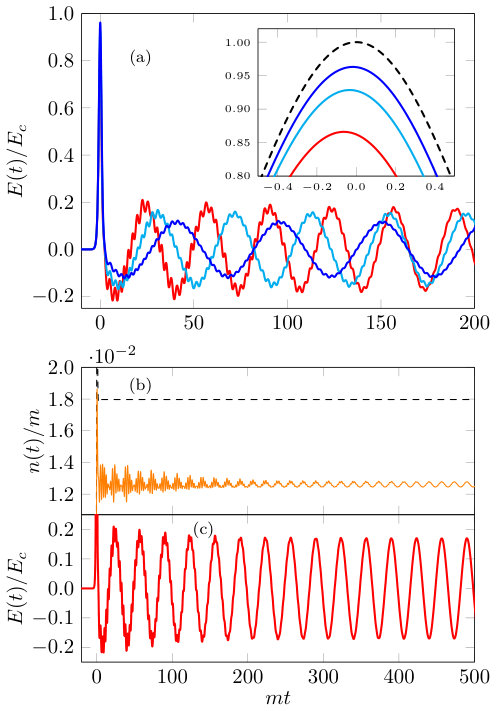 Figure 0
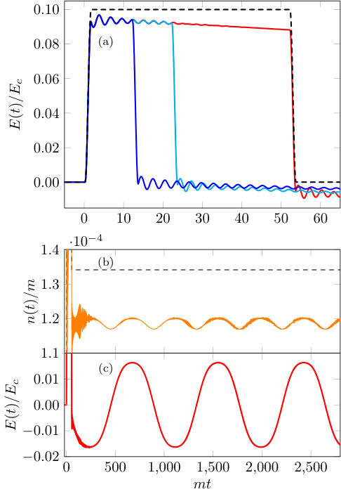 Figure 1
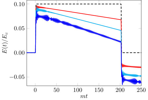 Figure 2
Peer Reviews
No public reviews on file for this paper yet. If you reviewed it on a platform where reviews are public (OpenReview, ICLR, NeurIPS, ICML), you can paste yours below so the community can read it here.
Videos
No videos yet. Explain this paper in a talk, walkthrough, or lecture? Add one.
\NewEnviron
alignt
[TABLE]
Response of the QED(2) Vacuum to a Quench:
Long-term Oscillations of the Electric Field and the Pair Creation Rate
A. Otto, D. Graeveling, B. Kämpfer
Institute of Radiation Physics, Helmholtz-Zentrum Dresden-Rossendorf,
01328 Dresden, Germany
Institut für Theoretische Physik, Technische Universität Dresden,
01068 Dresden, Germany
(March 6, 2024)
Abstract
We consider – within QED(2) – the backreaction to the Schwinger pair creation in a time dependent, spatially homogeneous electric field. Our focus is the depletion of the external field as a quench and the subsequent long-term evolution of the resulting electric field. Our numerical solutions of the self consistent, fully backreacted dynamical equations exhibit a self-sustaining oscillation of both the electric field and the pair number depending on the coupling strength.
\ioptwocol
1 Introduction
The Sauter-Schwinger effect is one of the most important examples of strong-field QED phenomena. It refers to the creation of electron-positron pairs by a spatially homogeneous electric field – the decay of the vacuum [1, 2] (cf. [3] for a recent review). A common picture is that virtual, entangled pairs constituting the vacuum are disrupted by the external electric field and lifted on the mass shell, thus loosing their entanglement in the long-time evolution. The rate at which pairs are created by an electric field of strength is . This rate is exceedingly small for macroscopic installations, since the Sauter-Schwinger (critical) field strength 1.3\text{\times}{10}^{18}\text{,}\mathrm{V}\mathrm{/}\mathrm{m}$$ is so large, while field strengths presently achievable in the lab are of the order of , which results in a huge suppression factor of . ( and the electron/positron mass and charge; we employ natural units with .)
Nonetheless one hopes upcoming high-intensity optical laser installations can provide the avenue towards the necessary fields. For lasers, the assumption of a constant electric field is not very realistic and a natural generalization is to let it be time dependent. This is called the dynamical Schwinger effect. The special case of a periodic field is dealt with in [4]. For ideas to boost the pair creation rate by superposing a strong, slowly varying field with a weak but fast field, see [5, 6].111 Multi-pair production is considered in [7].
For further generalizations to include spatial gradients, see [8, 9]. Other setups, not necessarily using lasers, are the field in the vicinity of a super-heavy atomic nucleus [10, 11, 12, 13, 14], or a superposed XFEL beam [15, 16]. For a survey of these effects, see [17]. Furthermore, ideas have also been put forward to forgo the direct detection of the produced fermions and instead focus on secondary photon signatures [18, 19, 20, 21].
These investigations have one thing in common: They suppose the electric (or more generally electro-magnetic) field has no dynamics of its own and is thus unaffected by the created pairs. However, physical intuition suggests the electrons and positrons will produce a current which will in turn generate a counter-acting electro-magnetic field that gets added to the original one. One calls this the backreaction of the fermions on the Maxwell field. Because the Schwinger pair production rate is already strongly suppressed for , the study of this further diminishing effect was postponed in favor of searching for amplification effects. But since the backreaction is of principal interest in its own right in illuminating the non-perturbative character of the Schwinger effect, we reconsider it in this paper in the context of QED (QED(2), also called the massive Schwinger model [22]). Backreactions were considered within QED(2) in [23, 24, 25].
A self consistent description of the backreaction is thus needed. This was first accomplished e.g. in [26, 27, 28, 29]. In the present contribution we build on theirs and extend it to investigate the long term evolution of the electric field and to investigate how the backreaction affects the created pairs. Put in a nutshell, we consider the response of the QED(2) vacuum to a quench caused by an external electric field.
2 Quantum kinetic equations with backreaction
We use the framework of the quantum kinetic equations, and our derivation follows [30, 31]. Incorporating the backreaction is done similarly to [29]. Our starting point is the Dirac equation in dimensions, . The gamma matrices are chosen as \gamma^{0}=\smallmatrixquantity(0&1\\ 1&0) and \gamma^{1}=\smallmatrixquantity(0&1\\ -1&0). Since our background field is assumed to be spatially homogeneous, an ansatz for via a Fourier transform, reduces the Dirac equation to a Schrödinger form {alignt} & i˙ψ(t,p) = h(t,p)ψ(t,p),
h(t,p) = (-p+eA(t) mm p-eA(t)).
The Hamiltonian has two time dependent eigenvectors , to the eigenvalues with . Two linearly independent solutions to the Dirac equations are obtained via the ansatz {alignt} u(t,p) &= α(t,p)U(t,p) + β(t,p)V(t,-p),
v(t,-p) = -β^(t,p)U(t,p) + α^(t,p)V(t,-p)
with , resulting in equations for and : {alignt} ˙α= -iΩα+ eEm2Ω2β, ˙β= -eEm2Ω2α+ iΩβ.
To get to observable quantities, we pass over to second quantization by promoting to an operator on Fock space. Since we have two bases (, and , ) at our disposal, we can expand in both: {alignt} ψ(t,p) &= c(p)u(t,p) + d^†(-p)v(t,-p)
= C(t,p)U(t,p) + D^†(t,-p)V(t,-p).
The relation between , and , follows from (2) as {alignt} C(t,p) &= α(t,p)c(p) - β^*(t,p)d^†(-p),
D^†(t,-p) = β(t,p)c(p) + α^*(t,p)d^†(-p),
which is called the Bogoliubov transform. Both sets of operators are fermionic creation/annihilation operators. The vacuum is annihilated by , , and the number of produced pairs is . This lets us define the total pair number {alignt} n(t) = ∫dp2π |β(t,p)|^2.
The second-quantized Hamiltonian is and when we normal order it in terms of and (indicated by ) we get {alignt} ∙H ∙ = ∫dp2πΩ[C^†C + D^†D].
Its expectation value, the energy of the vacuum, is . The factor is the volume of the system and divergent because of the homogeneity.
The particles produced by the electric field will induce a current . We denote by its mean field part the normal ordered expectation value which will be constant in , again due to the homogeneity. It evaluates to and {alignt} ¯j^1 = 2e∫dp2π [|β|^2 p-eAΩ- Re(α^*β)mΩ].
Note that without normal ordering w.r.t. , , , which is unphysical since the external field cannot create a net charge. Also normal ordering w.r.t. , would yield . This is also unphysical as the particles would not create a (spatial) current.
To this (internal) mean field current we add an arbitrary external current , which generates the external electric field (that is the quench) and plug both into Maxwell’s equation: {alignt} ˙E &= ˙E_ext- 2e∫dp2π [|β|^2 p-eAΩ- Re(α^*β)mΩ],
˙A = -E.
An alternative way of arriving at this equation, pursued in [29], is to start with the total energy density of the system {alignt} ϵ= E22 + 2∫dp2π |β|^2 Ω- ∫dt ˙E_extE
and setting . The last term is the work the external current must do to counteract the electric field. We use the energy density to check the accuracy of the numerics.
Whichever way one chooses, the equations (2) and (2) together with the initial conditions {alignt} &α(t_0, p) = 1, β(t_0, p) = 0, A(t_0) = 0,
E(t_0) = E_ext(t_0) = 0
form a well defined system of coupled ordinary differential equations that we are going to evaluate. Note that without the integral incorporating the backreaction in (2), the different momentum modes would be decoupled.
In dimensions, the coupling strength has dimension . The fine structure constant is then defined as and we give its value when specifying the strength of the backreaction.
3 Schwinger pair production for various pulse shapes
We will employ two different quenches caused by external electric fields.
3.1 Sauter pulse
The first is the so called Sauter pulse {alignt} E_ext(t) = E0cosh2(t/τ).
Note the initial condition can only be approximately fulfilled, but to arbitrary precision by choosing sufficiently large.
In figure 1(a) we show the time evolution of the electric field, determined by (2), with the Sauter pulse (3.1) as external field . The first spike is closely following . After the latter has faded away, starts to settle into a superposition of oscillations. These have already been noted in [28, 29], and were also found in [32] using different methods, where the Maxwell field was calculated using statistical averages, and in [33], using matrix product states. In [34], a similar effect was found without a driving external field, which the authors call plasmons in QED vacuum and attribute to the vacuum charge polarization. The inset in figure 1(a) shows a zoom to the peak of the electric field around . Increasing the coupling strength screens the electric field more, resulting in a lower net maximum; i.e. the electric field is depleted (cf. [35]). Increasing also increases both the frequency and amplitude of the oscillations.
Figure 1(c) shows the long-term evolution of the electric field . For the red curve, one can see that the oscillations with higher frequencies are transient, and the smaller wiggles vanish. This is also the case for the other curves, but harder to see. We conclude that after a short quench by the transient Sauter pulse the system does not return to its initial state, but rather the electric field keeps oscillating with a constant frequency and amplitude, looking like an eternal wobbling. The pair number (see figure 1(b)) oscillates in a similar manner as the electric field. Both subsystems are coupled through the total energy conservation (2). Switching off the backreaction, i.e. ignoring the integral in (2), yields no oscillations after the external field declines to zero, with both and constant.
3.2 Flat-top pulse
The second pulse shape we employ is a pulse with the following properties: {alignt} E_ext(t) = {0, t ≤0,E0, tr≤t ≤tr+tf,0, t ≥2tr+tf,
and monotonously increasing/decreasing where not specified. Its precise construction can be found in the appendix. In contrast to the Sauter pulse, it has two time scales, the ramping time over which the electric field is switched on and off, and the flat top time over which it is constant. The case captures the plain222 Rather a modified version, where the electric field does not extend to the infinite past, but gets turned on smoothly at some time.
Schwinger effect, but with the additional backreaction. The backreaction again causes some depletion, as evidenced in figure 2(a):
The electric fields grows to almost the value of the external field, enters some transient oscillations, and then drops, synchronized with the drop of the external field. Subsequently the field seemingly displays a similar eternal wobbling as in the long-time regime of the Sauter quench, see figure 2(c). The pair number’s oscillations (figure 2(b)) are also synchronized with the field oscillations.
The depletion can be more clearly seen in figure 3, where we plot the electric field for a longer lasting pulse and for varying . The sudden change in the external field lifts the total field but also induces transient oscillations. Once the external field is constant, the total field starts declining with a slope that grows as does, while the oscillations tend to zero (but observe that they take longer to do so for larger coupling strengths). The switching-off of the external field makes the total field swing in the oppsite direction after which it enters the long-term oscillating state exhibited in figure 2(c). Note that per (2) the external field does not add energy to the system for . Thus in the flat-top section the energy just gets shifted from the electric field to the created fermions.
4 Summary
In summary we consider the impact of the backreaction on Schwinger type pair creation. The produced pairs screen the external field and facilitate its net depletion. Viewing the external field as a quench to the vacuum, it is interesting to see the vacuum response as a wobbling of the number of created pairs in phase with the long-term oscillations of the induced electric field. For the selected examples and within the considered time intervals, the vacuum looks like an eternally swinging medium. Due to numeric reasons (see the momentum integral in (2)) we worked in dimensional QED, i.e. QED(2). The swinging vacuum response, however, seems to be generic, as the examples in [28, 29, 32, 33, 34] show.
Acknowledgments: The authors gratefully acknowledge inspiring discussions with R. Schützhold, H. Gies, R. Alkofer, D. B. Blaschke and C. Greiner. Many thanks go to S. Smolyansky and A. Panferov for previous common work on the plain Schwinger process. The fruitful collaboration with R. Sauerbrey and T. E. Cowan within the HIBEF project promoted the present investigation.
Appendix A Construction of the pulse
To construct the pulse shape for the electric field (3.2) we use a procedure often employed in differential geometry for partitions of unity, see e.g. chapter 13 in [36].
First define {alignt} r(x) = {0, x ≤0,e-1x, x > 0.
This function is but not analytic, since . Using it, define . Observe and . This lets us define {alignt} E_ext(t) = E_0s(ttr)s(2tr+tf-ttr)
which has all the properties we claimed for in (3.2).
The reference list from the paper itself. Each links out to its DOI / PubMed record.
- 1[1] F. Sauter “Über das Verhalten eines Elektrons im homogenen elektrischen Feld nach der relativistischen Theorie Diracs” In Z. Phys. 69.11 Springer-Verlag, 1931, pp. 742
- 2[2] J. Schwinger “On Gauge Invariance and Vacuum Polarization” In Phys. Rev. 82 , 1951, pp. 664
- 3[3] F. Gelis and N. Tanji “Schwinger mechanism revisited” In Prog. Part. Nucl. Phys. 87 , 2016, pp. 1–49
- 4[4] E. Brezin and C. Itzykson “Pair Production in Vacuum by an Alternating Field” In Phys. Rev. D 2.7 , 1970, pp. 1191–1199 DOI: 10.1103/Phys Rev D.2.1191 · doi ↗
- 5[5] R. Schützhold, H. Gies and G. Dunne “Dynamically Assisted Schwinger Mechanism” In Phys. Rev. Lett. 101.13 , 2008, pp. 130404 DOI: 10.1103/Phys Rev Lett.101.130404 · doi ↗
- 6[6] G. V. Dunne, H. Gies and R. Schützhold “Catalysis of Schwinger vacuum pair production” In Phys. Rev. D 80.11 , 2009, pp. 111301 DOI: 10.1103/Phys Rev D.80.111301 · doi ↗
- 7[7] Wöllert A, H. Bauke and C. H. Keitel “Multi-pair states in electron-positron pair creation” In Phys. Lett. B 760 , 2016, pp. 552–557
- 8[8] H. Gies and G. Torgrimsson “Critical Schwinger Pair Production” In Phys. Rev. Lett. 116 , 2016, pp. 090406