Semi-Levy driven continuous-time GARCH process
M. Mohammadi, S. Rezakhah, N. Modarresi

TL;DR
This paper introduces the semi-Levy driven continuous-time GARCH (SLD-COGARCH) process, characterizing its properties, stationarity conditions, and periodic correlation, with applications to high-frequency financial data modeling.
Contribution
The paper develops the SLD-COGARCH model, providing theoretical conditions for stationarity and demonstrating its periodic correlation properties and practical data fitting.
Findings
SLD-COGARCH process exhibits strict periodic stationarity under certain conditions.
Increments of SLD-COGARCH are periodically correlated, confirmed by simulation tests.
Model effectively fits high-frequency financial data.
Abstract
We study the class of semi-Levy driven continuous-time GARCH, denoted by SLD-COGARCH, process. The statistical properties of this process are characterized. We show that the state process of such process can be described by a random recurrence equation with the periodic random coeffcients. We establish sufficient conditions for the existence of a strictly periodically stationary solution of the state process which causes the volatility process to be strictly periodically stationary. Furthermore, it is shown that the increments with constant length of such SLD-COGARCH process are themselves a discrete-time periodically correlated (PC) process. We apply some tests to verify the PC behavior of these increments by the simulation studies. Finally, we show that how well this model fits a set of high-frequency financial data.
Click any figure to enlarge with its caption.
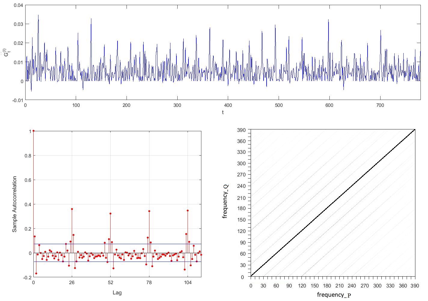 Figure 1
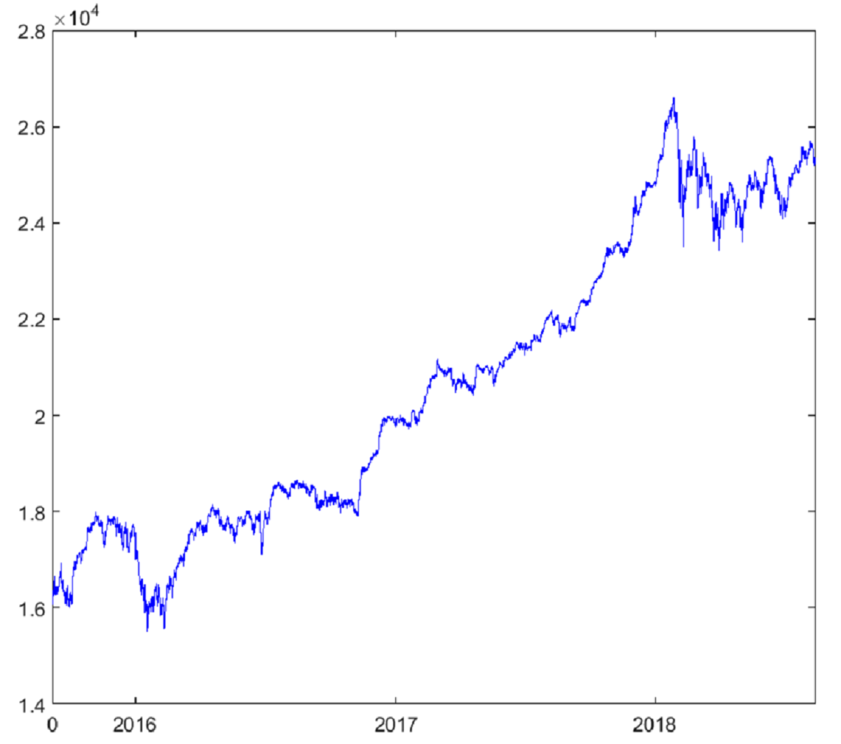 Figure 2
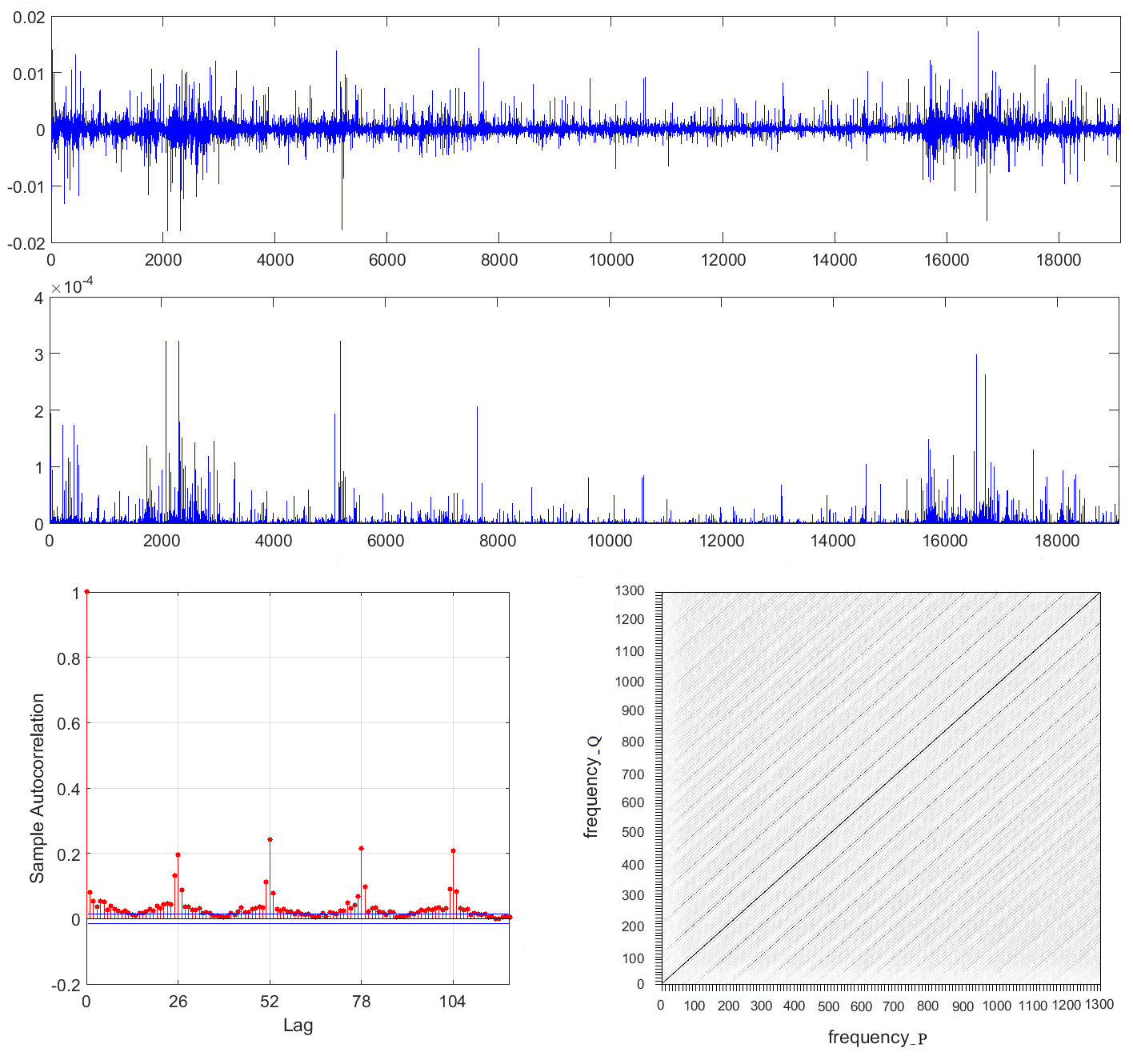 Figure 3
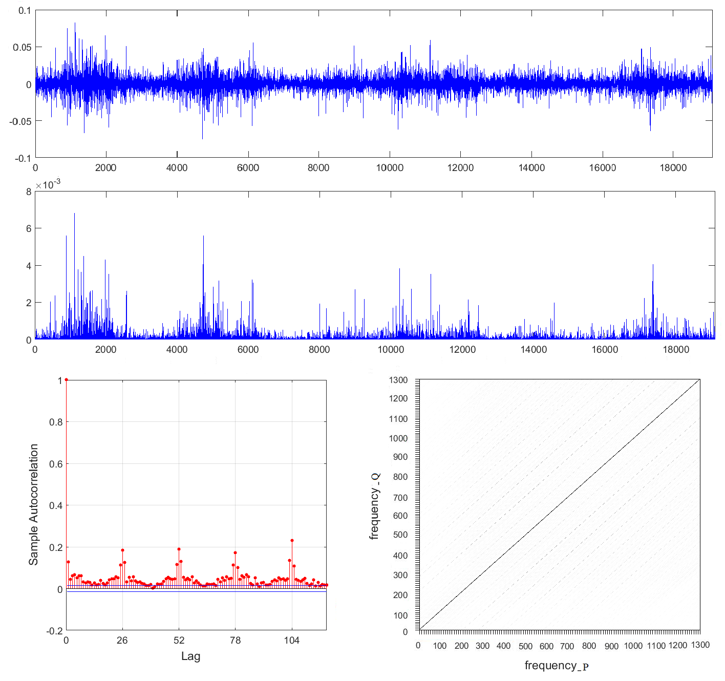 Figure 4
Peer Reviews
No public reviews on file for this paper yet. If you reviewed it on a platform where reviews are public (OpenReview, ICLR, NeurIPS, ICML), you can paste yours below so the community can read it here.
Videos
No videos yet. Explain this paper in a talk, walkthrough, or lecture? Add one.
Taxonomy
TopicsFinancial Risk and Volatility Modeling · Complex Systems and Time Series Analysis · Stochastic processes and statistical mechanics
Semi-Lévy driven continuous-time GARCH process
M. Mohammadi
Faculty of Mathematics and Computer Science, Amirkabir University of Technology, Tehran, Iran. E-mail: [email protected](M. Mohammadi) and [email protected](S. Rezakhah).
S. Rezakhah*∗*
N. Modarresi
Department of Mathematics and computer science, Allameh Tabataba’i University, Tehran, Iran. E-mail: [email protected](N. Modarresi).
Abstract
In this paper, we study the class of semi-Lévy driven continuous-time GARCH, denoted by SLD-COGARCH, process. The statistical properties of this process are characterized. We show that the state process of such process can be described by a random recurrence equation with the periodic random coefficients. We establish sufficient conditions for the existence of a strictly periodically stationary solution of the state process which causes the volatility process to be strictly periodically stationary. Furthermore, it is shown that the increments with constant length of such SLD-COGARCH process are themselves a discrete-time periodically correlated (PC) process. We apply some tests to verify the PC behavior of these increments by the simulation studies. Finally, we show that how well this model fits a set of high-frequency financial data.
AMS 2010 Subject Classification: 60G12, 62M10, 60G51, 60J75, 91B70, 93E15.
Keywords: continuous-time GARCH process; semi-Lévy process; strictly periodically stationary; periodically correlated.
1 Introduction
The discrete-time ARCH and GARCH processes are often applied to model financial time series [7, 1]. Kluppelberg et al. [10] introduced a continuous-time version of the GARCH(1,1), called COGARCH(1,1), process which has the potential to have a better description of changes by determining the underling continuous structure. The examples of such underling structure are Lévy processes like Brownian motion and Poisson process. They studied Lévy driven COGARCH(1,1) processes where noises are considered as increments of some Lévy process and proved the stationarity and also second order properties, under some regularity conditions. Brockwell et al. [4] generalized the Lévy driven COGARCH(1,1) process to the higher order. They defined the COGARCH() process driven by a Lévy process as the solution to the stochastic differential equation
[TABLE]
where the volatility process is a continuous-time ARMA(), called CARMA (), process. They presented the state-space representation of the volatility process as (see e.g. [3])
[TABLE]
and
[TABLE]
where is the discrete part of the quadratic variation process (see Protter [12, p.66]), and
[TABLE]
with and . They showed that the state process can be expressed as a stochastic recurrence equation with the random coefficients. Under some sufficient conditions, they proved that the volatility process is strictly stationary which causes the increments with constant length of the process to be stationary.
The Lévy driven COGARCH processes have the restriction that the relevant underling process has the stationary increments. In contrast with such stationary increment processes, processes with periodically stationary increments have a wider application. For example, the accumulated compensation claims from an insurance company in many cases have periodic increments. Specifically, car insurance companies are dealt with more accidental claims at the starting of the new year and in summer than the other parts of the year. As another example, the precipitation in almost all parts of the world have periodic behavior and so the volume of underground waters are higher in some months and lower in some months in each year. The observations of such time series have significant dependency to the previous periods as well. Motivated by these observations, the underling processes with periodically stationary increments, say semi-Lévy processes, are more prominent than the Lévy processes. So, we study semi-Lévy driven COGARCH, denoted by SLD-COGARCH, process in this paper. The semi-Lévy processes have been extensively studied by Maejima and sato [11]. Recognizing such semi-Lévy processes often can be followed by considering some fixed partitions of the corresponding period where inside successive partitions the process has different Lévy type structure and has similar structure to the corresponding element of the previous periods.
In this paper, we study the statistical properties of the SLD-COGARCH() process. Providing a random recurrence equation with periodic random coefficients for the state process defined by (1.2), we show that it converges almost surely under some regular conditions. We establish sufficient conditions for the existence of a strictly periodically stationary solution of the state process which causes the volatility process defined by (1.1) to be strictly periodically stationary. Furthermore, the increments with constant length of the SLD-COGARCH() process are a discrete-time periodically correlated (PC) process. We use some tests to verify the PC behavior of the increments. Finally, we apply the introduced model to some real data set.
This paper is organized as follows. In section 2, we introduce the SLD-COGARCH processes. We also present the structure of the semi-Lévy process and obtain its characteristic function. Section 3 is devoted to some sufficient conditions that cause the volatility process to be strictly periodically stationary. We also show that the increments with constant length of such SLD-COGARCH process form a PC process. In section 4, we illustrate the results with simulations. In section 5, we apply the model to a set of high-frequency financial data and show that this process has the consistent properties. All proofs are presented in Section 6.
2 Semi-Lévy driven COGARCH process
In this section, we describe the structure of semi-Lévy compound Poisson process in subsection 2.1. Following the method of Brockwell et al. [4], we present the structure of corresponding semi-Lévy compound Poisson process as the underling process of the COGARCH process in subsection 2.2.
2.1 Semi-Lévy process
We present the definition of semi-Lévy Poisson and semi-Lévy compound Poisson processes. Then, we drive the characteristic function of the semi-Lévy compound Poisson process.
Definition 2.1
**(Semi-Lévy Poisson process)
**Let where constitutes a partition of positive real line and for some integer and all and also . Then, a non-homogeneous Poisson process \big{(}N(t)\big{)}_{t\geq 0} is called a semi-Lévy Poisson process with period and intensity function if E\big{(}N(t)\big{)}=\Lambda(t) where
[TABLE]
and for and .
One can easily verify that a semi-Lévy Poisson process has periodically stationary increments.
Definition 2.2
**(Semi-Lévy compound Poisson process)
**Let \big{(}N(t)\big{)}_{t\geq 0} be a semi-Lévy Poisson process with some period . Then, the semi-Lévy compound Poisson, denoted by SLCP, process is defined as
[TABLE]
where and in which is the arrival time of jump , and are independent and identically distributed (i.i.d.) random variables with distribution , such that .
The characteristic function of this process is derived from the following Lemma.
Lemma 2.1
Let be the SLCP process introduced by Definition 2.2. Then its characteristic function has the following Lévy-Khintchine representation
[TABLE]
where
[TABLE]
and
[TABLE]
in which and .
Proof: see Appendix, P1.
Remark 2.1
(i) By the fact that the numbers of jumps of the SLCP process in the time interval are finite and the size of each jump is finite as well, we deduce that the process is a finite variation process, see [13, p.14]. Hence, the process is a semimartingale [12, p.55].
(ii) By Definition 2.2, we have that if there is a jump at point , , then
[TABLE]
otherwise . Thus, by the Theorem 22 of Protter [12, p.66], if there is a jump at point then and otherwise . So, the quadratic variation of the process is given by
[TABLE]
2.2 Semi-Lévy driven COGARCH process
The representation of the Lévy driven COGARCH() process is based on the structure of the GARCH() process as
[TABLE]
where and is a sequence of i.i.d. random variables. The process can be interpreted as the log return of the asset price process , say . The volatility process is as an ARMA() process driven by the noise sequence . Motivated by this, the dynamic of the Lévy driven COGARCH() process for the logarithm of the asset price process is defined as
[TABLE]
where is a Lévy process and is a continuous-time analog of the self-exciting ARMA() process , see Brockwell et al. [4].
We generalize the Lévy driven COGARCH() process by replacing the Lévy process with the SLCP process .
Definition 2.3
**(SLD-COGARCH())
**Let be the SLCP process with some period defined by (2.2). Then the left-continuous volatility process is defined as
[TABLE]
where the state process is the unique càdlàg solution of the stochastic differential equation
[TABLE]
with an initial value which is independent of the driving process , in which is the quadratic variation of the process and the ()-matrix and vectors and are defined as
[TABLE]
*where and are integers such that and .
If the volatility process defined by (2.6) is almost surely non-negative, then given by*
[TABLE]
is called the SLCP driven COGARCH(p,q), denoted by SLD-COGARCH(p,q), process with parameters , , and the driving process .
We present the definition of matrix norms and some notation that will be used throughout the paper.
Definition 2.4
Let denote the vector -norm in , for . Then the matrix -norm of the matrix is defined as
[TABLE]
The matrix -norms of the , and are called the maximum absolute column sum norm, spectral norm and maximum absolute row sum norm, respectively.
Definition 2.5
Let be a matrix such that is a diagonal matrix, where B is defined by (2.8). Then the natural matrix norm of is
[TABLE]
The natural matrix norm corresponding to the natural vector norm is defined as
[TABLE]
The eigenvalues of the matrix B are denoted by and , where is the real part of the eigenvalue . The ()-identity matrix is denoted by or simply .
3 Periodic stationarity of the increments
In this section, we show that under some conditions, the volatility process defined by (2.6) is strictly periodically stationary with period . The increments with constant length of the SLD-COGARCH process are a periodically correlated (PC) process. Furthermore, under a necessary and sufficient condition, the volatility process is non-negative.
The following theorem shows that the state process of the SLD-COGARCH process defined by (2.7) satisfies a multivariate random recurrence equation with periodic random coefficients.
Theorem 3.1
Let be the state process of the SLD-COGARCH process. Then the following results are hold.
- (a)
*There exists a random *matrix and a random vector such that
[TABLE]
- (b)
\big{(}J_{s,t},\mathbf{K}_{s,t}\big{)}* are periodic in both indices with the same period . So, the distribution of \big{(}J_{s,t},\mathbf{K}_{s,t}\big{)} is invariant under time changes of to .*
- (c)
\big{(}J_{s,t},\mathbf{K}_{s,t}\big{)}* and \big{(}J_{r,u},\mathbf{K}_{r,u}\big{)} are independent for . is also independent of \big{(}J_{s,t},\mathbf{K}_{s,t}\big{)}.*
Proof: see Appendix, P2.
In the next theorem, we consider some mild conditions to the state process that converges in distribution to a finite random vector.
Theorem 3.2
Let be the state process of the SLD-COGARCH process that is satisfied in the followings
- (i)
all the eigenvalues of the matrix B are distinct and have strictly negative real parts,
- (ii)
there exists some such that for and
[TABLE]
where is a matrix which causes is diagonal.
Then, for the fixed , converges in distribution to some vector , as . Furthermore, has a unique distribution that is satisfied in equation
[TABLE]
where denotes the equality in distribution and is independent of \big{(}J_{t,t+\tau},\mathbf{K}_{t,t+\tau}\big{)}.
Proof: see Appendix, P3.
Corollary 3.3
Under the conditions (i) and (ii) of Theorem 3.2, the following results are hold.
- (a)
If for any , then and defined by (2.6) are strictly periodically stationary with the period . In other words, for any and
[TABLE]
and
[TABLE]
- (b)
Increments with the constant length of the SLD-COGARCH process is a PC process. In other words, for any and fixed satisfies
[TABLE]
and
[TABLE]
Proof: see Appendix, P4.
One of the striking features of high-frequency financial data is that the returns have negligible correlation while the squared returns are significantly correlated. These data typically show a PC structure in their squared logarithm returns (known as squared log return). The next corollary shows that under some conditions, the increments with constant length of the SLD-COGARCH which were defined in Corollary 3.3 (b) can capture these features.
Corollary 3.4
Let the conditions of Theorem 3.2 hold and the driving process defined by (2.2) has zero mean. Then increments with constant length for and satisfies
[TABLE]
Proof: see Appendix, P5.
The following theorem represents the necessary and sufficient conditions for non-negativity of the volatility process for any .
Theorem 3.5
Let be the state process of the SLD-COGARCH process with parameters , and . Suppose that be a real constant that satisfies in
[TABLE]
and
[TABLE]
*Then, with probability one, for .
Conversely, if either (3.5) fails or (3.5) holds with and (3.4) fails, then there exists a SLCP process and such that .*
Proof: see Appendix, P6.
4 Simulation
In this section, we verify the theoretical results concerning the PC structure of the increments of the SLD-COGARCH process is defined in (2.9) through the simulation. For this, we first simulate the driving semi-Lévy process with period introduced by Definition 2.2. Second, we present the discretized version of the state process defined by (2.7) at the time of jump points. We generate the volatility process defined by (2.6) and the process at the time of jump points. Then, we evaluate a sampled process from the simulated values of the process . Finally, we apply some tests to demonstrate the PC structure of the increments for the sampled process.
For simulating the driving process with the underlying semi-Lévy Poisson process \big{(}N(t)\big{)}_{t\geq 0}, we consider as the time of jump \big{(}N(t)\big{)}_{t\geq 0} and . First, by Definition 2.1, we generate the arrival times of the process \big{(}N(t)\big{)}_{t\geq 0} by the following algorithm.
Consider the positive value as the length of the period of the process and some integer as the number of period intervals for the simulation. 2. 2.
Choose the positive integer as the number of elements of partition in each period interval. 3. 3.
Consider positive real numbers such that and a partition of first period interval by where , and , . Elements of partition of period interval \big{(}(k-1)\tau,k\tau\big{]} are where for and . 4. 4.
Let the positive real numbers be occurrence rates corresponding to the increments of on . It is also followed from Definition 2.1 that the process has the occurrence rate on for and . 5. 5.
Generate an independent sequence of Poisson random variables with parameter on for as . 6. 6.
Generate independent samples from uniform distribution for . Then, sort these samples and denote these ordered samples by . 7. 7.
Generate the successive jump size independently and with distribution if corresponding arrival time belongs to for and evaluate by (2.2).
Now, by the following steps, we simulate the SLD-COGARH() process introduced by Definition 2.3.
Set integer valued and such that 2. 2.
Choose the real parameters and and such that , , . Furthermore, the eigenvalues of the matrix , , are distinct and have strictly negative real parts and conditions (3.2), (3.4) and (3.5) are satisfied.
To verify the condition (3.2), define the matrix as follows
[TABLE] 3. 3.
After generating the arrival times , by the above algorithm, generate the state process in (6.8) with an initial value
[TABLE] 4. 4.
Similar to (6.5) for can be written as . So, by (2.6), generate the process with
[TABLE] 5. 5.
Since the driving process has one jump at time over , it follows from (2.9) that
[TABLE]
Then generate the process by (4.2) such that . 6. 6.
Finally, using the values of and provided by the previous steps, evaluate the sampled processes and for where is some integer by the following steps:
- •
For , it follows from (6.5) that . So, using (2.6), we have
[TABLE]
Note that if , by (4.1)
[TABLE]
- •
Using the fact that the driving process has no jump over , for , it follows from (2.9) for
[TABLE]
Thus, . If , then it follows from (4.2) that
[TABLE]
To detect the PC structure of a process, it is shown that the proposed sample spectral coherence statistic can be used to test whether a discrete-time process is PC [8, 9]. In this method, for samples , and a fixed , the following sample spectral coherence statistic is plotted
[TABLE]
where , and for .
The perception of this sample spectral coherence is aided by plotting the coherence values only at points where the following threshold is exceeded [9, p.310]
[TABLE]
For a PC time series with period , it is expected that the sample spectral coherence statistic has a significant value on pairs for . The plot of the support of the sample spectral coherence statistic can be used to identify the type of model and analysis of the time series , see [6]:
- •
If only the main diagonal appears, then the time series is a stationary time series.
- •
If there are some significant values of statistic and they seem to lie along the parallel equally spaced diagonal lines, then the time series is PC with period , where is the line spacing.
- •
If there are some significant values of statistic but they occur in some non-regular places, then the time series is a non-stationary time series.
In the following, we provide an example to investigate the process.
Example 4.1
Let be a SLCP process with period . Furthermore, the lengths of the successive subintervals of each period interval are 0.5, 2.5, 3, 0.5 where corresponding occurrence rates of the semi-Lévy Poisson process on these subintervals are assumed as 4, 10, 5, 30. Moreover, the distribution of jump sizes on these subintervals are N(2, 4), N(1.5, 2.5), N(2.5, 1.5) and N(1.75, 3), where denotes a Normal distribution with mean and variance . In this example, we consider SLD-COGARCH(1,3) process with parameters , , , and . Thus, the matrix is
[TABLE]
and conditions (3.2), (3.4) and (3.5) are satisfied. For such SLD-COGARCH process, we simulate for the duration of period intervals by the specified parameters, and by the suggested simulation algorithm. Then, by the step 6 of the last algorithm, we get equally space samples with length . So, we have 780 discretized samples of this 30 period intervals.
In Figure 1, we see the differenced series (top) and its sample autocorrelation (bottom left). The sample spectral coherence statistic of this series for a specified collection of pairs and that exceed the threshold corresponding to which is presented at the bottom right. If , then the parallel lines for the sample spectral coherence confirm the series is PC with period . This implies that, for ,
[TABLE]
and
[TABLE]
So, it follows from (4.5) and (4.6) that the series has a PC structure with period .
5 Real data analysis
One of the striking features of financial time series is that the log returns have negligible correlation while its square log returns are significantly correlated [4]. Many of these time series are collected at a high-frequency and typically show a PC structure in their squared log returns [14]. In this section, we evaluate the results of Corollary 3.4 and show that the SLD-COGARCH process can capture the periodic structure of high-frequency financial data. For this, we use the 15-minute log returns of the Dow Jones Industrial Average (DJIA) index.
This data set is recorded between 9:35 to 16:00 from September 4th, 2015 to August 14th, 2018. There was a total of 735 trading days not including the weekends and holidays with 26 15-minute observations per day, resulting in the total of n = 19110 15-minute observations. Figure 2, shows the DJIA index for the specified times.
In Figure 3, we show the 15-minute log returns of DJIA (top), their squares (middle) and sample autocorrelation function (ACF) of the squared log returns (bottom left). It is clear from ACF that 15-minute squared log returns have a seasonal structure with period 26. To show more precisely the PC structure of these data, we sample last 100 trading days. These data were recorded from March 22th, 2018 to August 14th, 2018 which contain 2600 observations. Then, we present the sample spectral coherence statistic of their squared log returns for a specified collection of pairs and . It is shown that it exceeds the threshold corresponding to in Figure 3 (bottom right). Therefore, sample spectral coherence statistic clearly shows that the squared log returns have a PC structure with period .
Currently we show that how well SLD-COGARCH process fits the 15-minute log returns of DJIA index. For this, we first simulate the driving process which is specified in Example 4.1 in the case that and the distribution of jump sizes are assumed to be N(0,4), N(0,2.5), N(0,1.5) and N(0,3). Second, we simulate the SLD-COGARCH(1,3) process for the duration of period intervals with the initial value and the parameters , , , and by the suggested simulation algorithm. Then, by the step 6 of the last algorithm, we get 19110 equally space samples by length .
Figure 4 shows the increments of the sampled process , (top) and their squares (middle) and ACF of the squared increments (bottom left). We select the last 2600 simulated data as sample and present the sample spectral coherence statistic of their squared increments for a specified collection of pairs and . It is shown that it exceeds the threshold corresponding to in Figure 4 (bottom right). The ACF and sample spectral coherence statistic demonstrate that the squared increments have a PC structure with period . Therefore, these graphs show that SLD-COGARCH process can be consistent with 15-minute log returns of DJIA index.
6 Appendix
**P1: Proof of Lemma 2.1
**For any there exist such that , where . So, it follows from Definition 2.1 and Definition 2.2 that
[TABLE]
Since, by Definition 2.2, the jump sizes are independent for , we have that
[TABLE]
By the fact that the jump sizes in each partition are i.i.d. random variables with distribution , it follows from Definition 2.1 and conditional expected value that
[TABLE]
where . The last equality follows from (2.1) and the fact that the semi-Lèvy Poisson process has the occurrence rate on for . An argument similar to that used in (6.2) shows that
[TABLE]
By replacing from (6.2) and (6.3) in (6.1), it reads as
[TABLE]
where
[TABLE]
P2: Proof of Theorem 3.1
Proof (): Let be the driving process introduced by Definition 2.2, be the time of jump and . Following the method of Brockwell et al. [4], and as has no jump over , it follows by (2.5) that for . So (2.7) implies that satisfies for . Hence
[TABLE]
and
[TABLE]
Integrating from to , we have that
[TABLE]
By (2.7) and (2.5), we have that has a jump of size at . So, at can be written as
[TABLE]
Integrating of (6.4) this time from to , we have that
[TABLE]
Therefore
[TABLE]
By assuming , (6.5) reads as
[TABLE]
and (6.8) as
[TABLE]
By successive replacement from (6.10) in (6.9) we have that
[TABLE]
Similar to (6.6) at can be written as
[TABLE]
By integrating of (6.4) from to , we have that
[TABLE]
Replacing this in (6.12) implies that
[TABLE]
By replacing from (6.13) in (6.11), it reads as
[TABLE]
Proof (b): We show that the distribution of and are periodic in both indices and , with the same period . Following the fact that and which are defined by (6.14) depend on and through
- •
the jump sizes ’s which by Definition 2.1 are independent and periodically identically distributed random variables with distribution ,
- •
which are inter-arrival times of which by Definition 2.1 has periodically stationary increment with period , So are periodic with period . Also are periodic by the same reason,
- •
is the current life at time which is periodic with period . Also is a function of which excess life and is periodic with period ,
it follows that
[TABLE]
So, are periodic in both indices and , with the same period .
Proof (c): By (6.14) it is clear that and are constructed from segments of the driving process in the intervals and , respectively. Thus and are independent for .
Now we show that is independent of \big{(}J_{s,t},\mathbf{K}_{s,t}\big{)}. By (6.14) we have that
[TABLE]
As and are independent and that is independent of the driving process , assumed by (2.7), it follows that and are independent.
**P3: Proof of Theorem 3.2
**For fixed and for , it follows from (6.14) that
[TABLE]
By successive replacement from (6.15) we obtain
[TABLE]
Since, by the part () of Theorem 3.1, are i.i.d., it follows from (6.16) that
[TABLE]
The following method of Brockwell et al. [4], for the proof of this theorem we use the general theory of multivariate random recurrence equations, see Bougerol and Picard [2]. For this, we first show that there exist some and matrix such that
[TABLE]
where . Then, it follows from the strong law of large numbers that the Lyapunov exponent of the i.i.d. sequence is strictly negative
[TABLE]
Therefore, as shown by Bougerol and Picard [2], the sum for all is converges almost surely (a.s.).
Since the eigenvalues of the matrix , , are distinct, we define the matrix as follows
[TABLE]
So, the matrix is the diagonal matrix with entries on the diagonal. Using the fact that is a invertible matrix, it follows from the exponential matrix definition that, for ,
[TABLE]
Hence, is the diagonal matrix with entries on the diagonal. Since the eigenvalues of the matrix B have strictly negative real parts, it follows from the Definition 2.5 that, for ,
[TABLE]
By denoting
[TABLE]
in (6.14) we have that
[TABLE]
So, by (6.19) we have that
[TABLE]
[TABLE]
so, (6.21) reads as
[TABLE]
Therefore
[TABLE]
So, it follows from (3.2) and (6.23) that
[TABLE]
To show that E\big{(}log^{+}||\mathbf{K}_{t,t+\tau}||_{P,r}\big{)}<\infty, observe from (6.14) and (6.20) that
[TABLE]
So, by (6.19) we have that
[TABLE]
The eigenvalues of the matrix B have strictly negative real parts, say . So, it follows that and for
[TABLE]
From this and (6.22) we have that
[TABLE]
Thus, (6.24) reads as
[TABLE]
Since E\big{(}Z_{i}^{2}\big{)}<\infty and E\big{(}N(t+\tau)-N(t)\big{)}=\Lambda(t+\tau)-\Lambda(t)<\infty, it follows that E\big{(}||\mathbf{K}_{t,t+\tau}||_{P,r}\big{)}<\infty. So, by Jensen’s inequality, we have that
[TABLE]
Now, since E\Big{(}log||J_{t,t+\tau}||_{P,r}\Big{)}<0 and E\Big{(}log^{+}||\mathbf{K}_{t,t+\tau}||_{P,r}\Big{)}<\infty, it follows from the general theory of random recurrence equations (see [2]) that , in (6.17), converges a.s. to 0 as and that converges a.s. absolutely to some random vector as , for fixed . Using the fact that the process has càdlàg paths, it follows that is a.s. finite for fixed . So
[TABLE]
and it follows the converges in distribution to as , for fixed .
It remains to show that satisfies (3.3) for fixed . It follows from (6.15) and the part (c) of Theorem 3.1 that is independent of , . So, by the fact that and are i.i.d., for any , and that converges in distribution to as , we have that
[TABLE]
where is independent of and denotes the convergence in distribution. Hence, by (6.15) and (6.25), it follows (3.3).
P4: Proof of Corollary 3.3
Proof (): By Theorem 3.2, is the long run behavior of for fixed and large , so that and is independent of . Since, by the part (b) of Theorem 3.1, and , for , are i.i.d., we have that
[TABLE]
It also follows from the parts () and (c) of Theorem 3.1 that, for fixed and ,
[TABLE]
and that is independent of . Thus if for , then (6.26) and (6.27) imply that . Further, it follows by induction on that
[TABLE]
We show that the process is strictly periodically stationary with period . If , then for any there exist and such that . So, by (6.28) we have that
[TABLE]
Now, let and . Since, by the part () of Theorem 3.1,
[TABLE]
it follows that is a Markov process. So, by the fact that , we have that
[TABLE]
Therefore, an induction argument for and (6.30) imply
[TABLE]
Hence, by (2.6) it follows that
[TABLE]
Proof (b): By (2.6) and (6.14) we have that
[TABLE]
As are constructed from segments of the driving process in the interval , see Theorem 3.1 (c), and that is independent of , assumed by (2.7), it follows that and are independent. So, (6.31) and semi-Lévy structure of imply that and both are periodic with the same period , say
[TABLE]
Thus it follows from (6.33) that
[TABLE]
and
[TABLE]
Hence, from (6.34) and (6.35) we have that
[TABLE]
P5: Proof of Corollary 3.4
Proof (): By the part (b) of Corollary 3.3, it follows that and are independent for any . So, and
[TABLE]
Since, by Definition 2.2, the jump sizes have finite second order moment it is easy to see that . So, it follows from the proposition 3.17 of Cont and Tankov [5] that is a martingale. Thus, from Itô isometry for square integrable martingales as integrators (e.g. Rogers and Williams [13], IV 27) follows
[TABLE]
for . Hence, cov\big{(}G_{t}^{(l)},G_{t+h}^{(l)}\big{)}=0.
Proof (b): By (6.33) we have that
[TABLE]
and
[TABLE]
Hence, from (6.36) and (6.37) it follows that
[TABLE]
**P6: Proof of Theorem 3.5
**Suppose that (3.4) and (3.5) both hold. The following proof of Theorem 3.1, for any it follows that . So, we have by (6.9) that
[TABLE]
By (2.6) and replacing from in , (6.6) reads as
[TABLE]
and (6.7) as
[TABLE]
Replacing (6.40) in (6.39) implies that
[TABLE]
So, it follows from (6.38) and (6.41) that
[TABLE]
By successive replacement from (6.41) in (6.42) we have that
[TABLE]
So, from this and (3.5) follows that
[TABLE]
By a similar method in Brockwell et al. [4], we find by (2.6) and (6.44) that for . It also follows from (6.44), (3.5) and (3.4) that
[TABLE]
So, by induction one can easily verify for any .
To prove the converse, suppose first that (3.5) fails. Then, it follows from (6.43) that, for ,
[TABLE]
Since , it follows from (6.45) and that for . Now assume that (3.5) holds with , but (3.4) fails. Suppose that the support of the jumps distribution is unbounded. Let be an interval such that for any and for some . By (2.6), (6.43) and (3.5) we have that
[TABLE]
It follows from (6.46) and assumption , that . So, one can easily verify that the set
[TABLE]
has positive probability for . On , by (6.43) we have that
[TABLE]
Since , by choosing large enough it follows from (6.47) that .
The reference list from the paper itself. Each links out to its DOI / PubMed record.
- 1[1] T. Bollerslev (1986). Generalized Autoregressive Conditional Heteroskedasticity. Journal of Econometrics, 31, 307–327.
- 2[2] P. Bougerol and N. Picard (1992). Stationarity of GARCH processes and of some nonnegative time series. Journal of Econometrics, 52, 115-127.
- 3[3] P.J. Brockwell (2009). Lévy-driven Continuous time ARMA processes. Handbook of Financial Time Series 457-480.
- 4[4] P.J. Brockwell, E. Chadraa and A. Lindner (2006). CONTINUOUS-TIME GARCH PROCESSES. Ann. Appl. Probab., 16(2), 790-826.
- 5[5] R. Cont and P. Tankov (2004). Financial Modelling With Jump Processes. Chapman and Hall/CRC Financial Mathematics Series.
- 6[6] A.E. Dudek, H. L. Hurd, W. Wojtowicz (2015). PARMA models with applications in R, Applied Condition Monitoring, Vol 3 (Cyclostationarity: Theory and Methods-II) Springer, Switzerland, 131-154.
- 7[7] R.F. Engle (1982). Autoregressive Conditional Heteroscedasticity with Estimates of the Variance of United Kingdom Inflation. Econometrica, 50, 987-1008.
- 8[8] H.L. Hurd, N.L. Gerr (1990). Graphical methods for determining the presence of periodic correlation. Journal of Time Series Analysis, 12(4), 337-350.