Finite State Machines for Semantic Scene Parsing and Segmentation
Hichem Sahbi

TL;DR
This paper presents a novel stochastic inference framework using finite state machines for semantic scene annotation and segmentation, enabling complex operations like reordering and label dependency modeling.
Contribution
It introduces a generative FSM-based approach that encodes annotation lattices and integrates multiple operations for improved scene parsing.
Findings
Effective scene annotation and segmentation
New FSM operations for reordering and label dependencies
Unified framework for multiple inference tasks
Abstract
We introduce in this work a novel stochastic inference process, for scene annotation and object class segmentation, based on finite state machines (FSMs). The design principle of our framework is generative and based on building, for a given scene, finite state machines that encode annotation lattices, and inference consists in finding and scoring the best configurations in these lattices. Different novel operations are defined using our FSM framework including reordering, segmentation, visual transduction, and label dependency modeling. All these operations are combined together in order to achieve annotation as well as object class segmentation.
Click any figure to enlarge with its caption.
 Figure 10
 Figure 11
 Figure 12
 Figure 13
 Figure 14
 Figure 15
 Figure 16
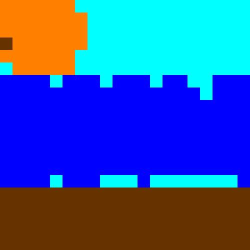 Figure 17
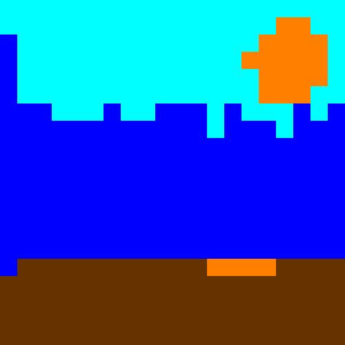 Figure 18
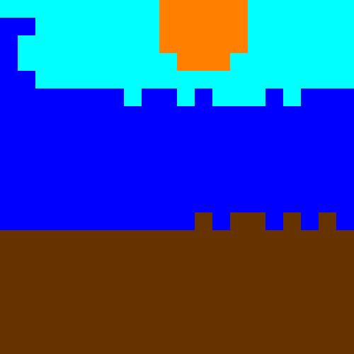 Figure 19
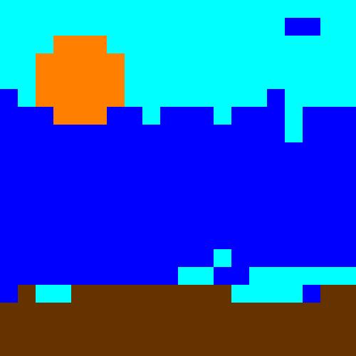 Figure 20
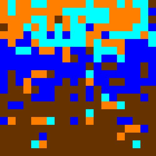 Figure 21
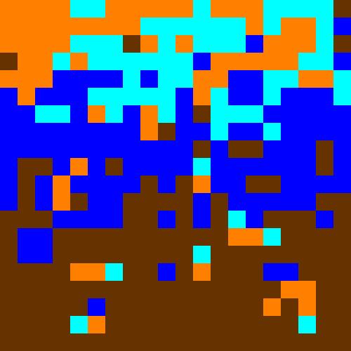 Figure 22
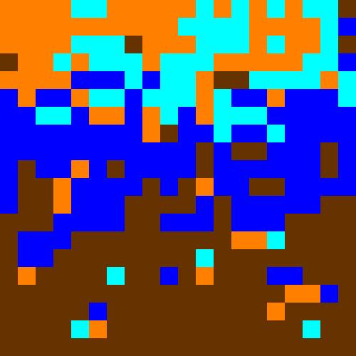 Figure 23
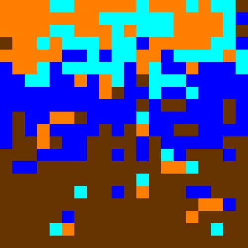 Figure 24
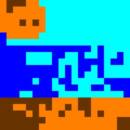 Figure 25
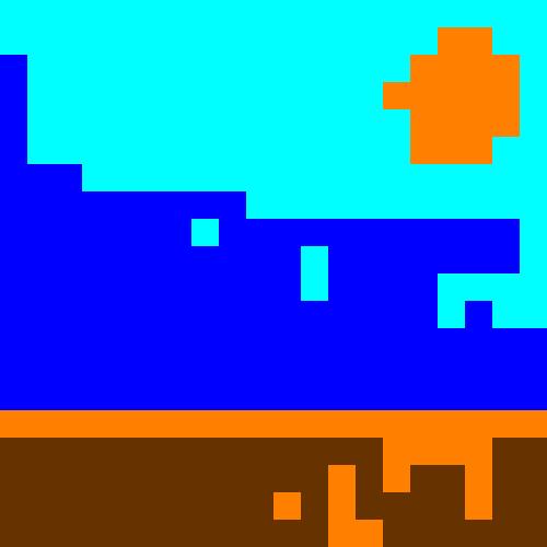 Figure 26
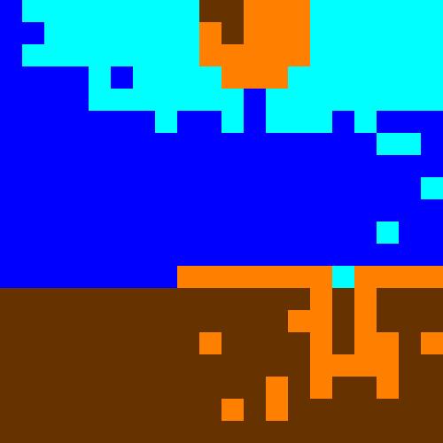 Figure 27
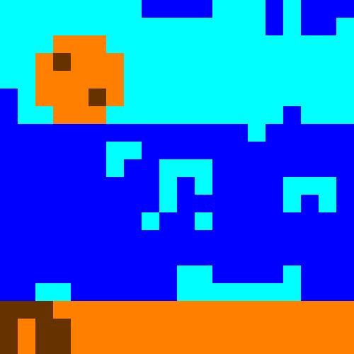 Figure 28
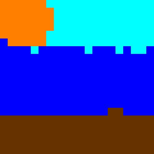 Figure 29
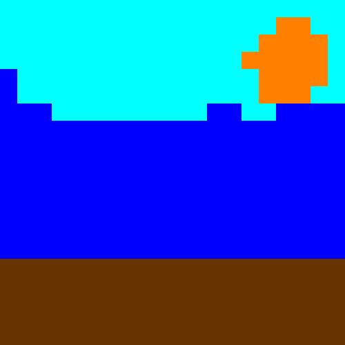 Figure 30
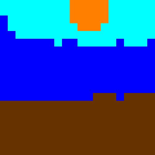 Figure 31
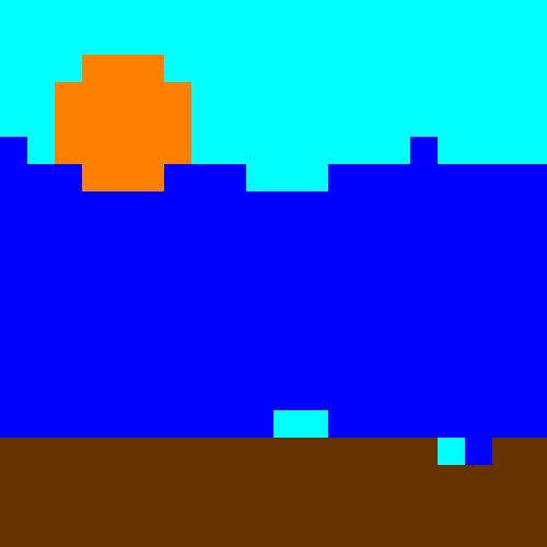 Figure 32
 Figure 33
 Figure 34
 Figure 35
 Figure 36
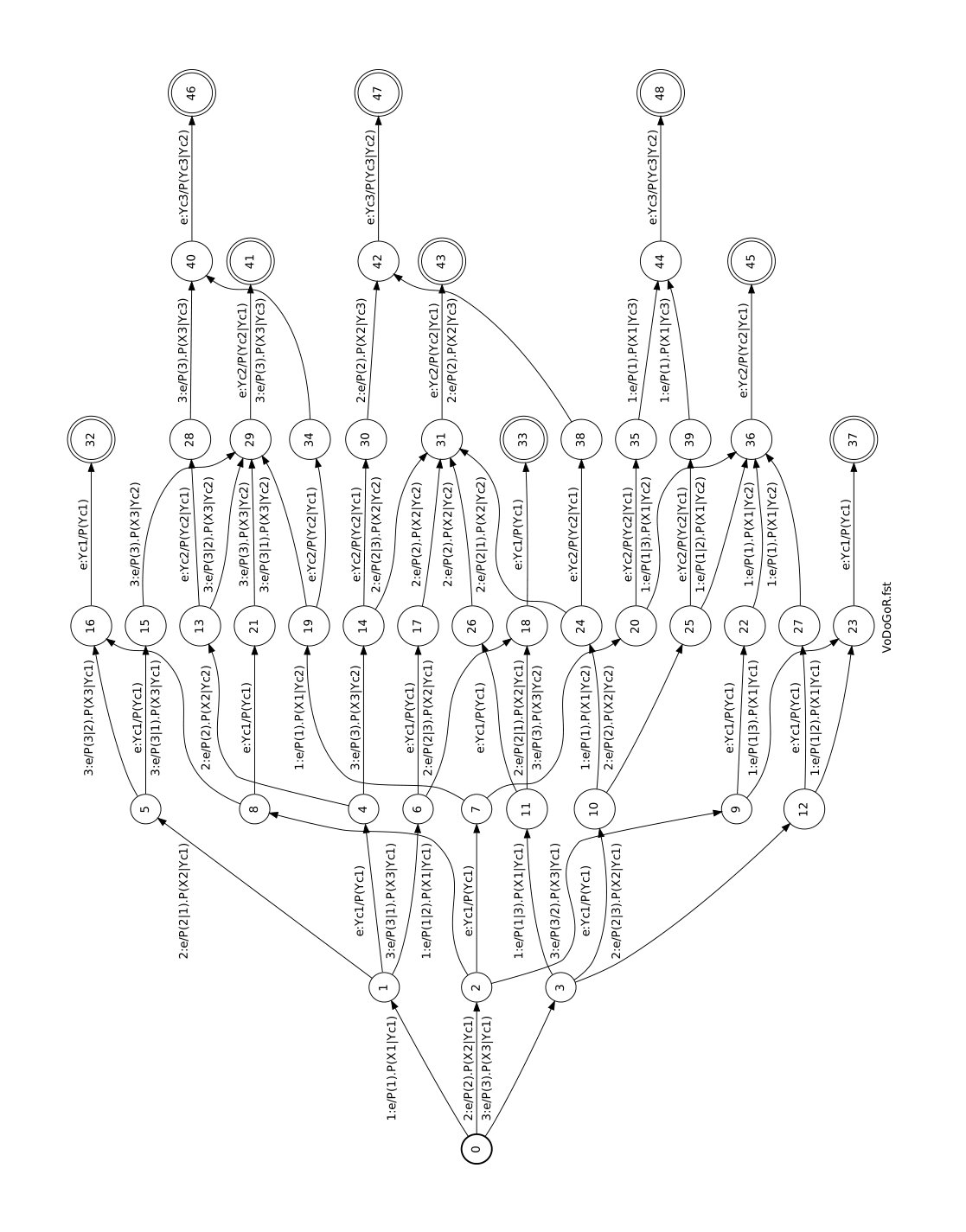 Figure 4
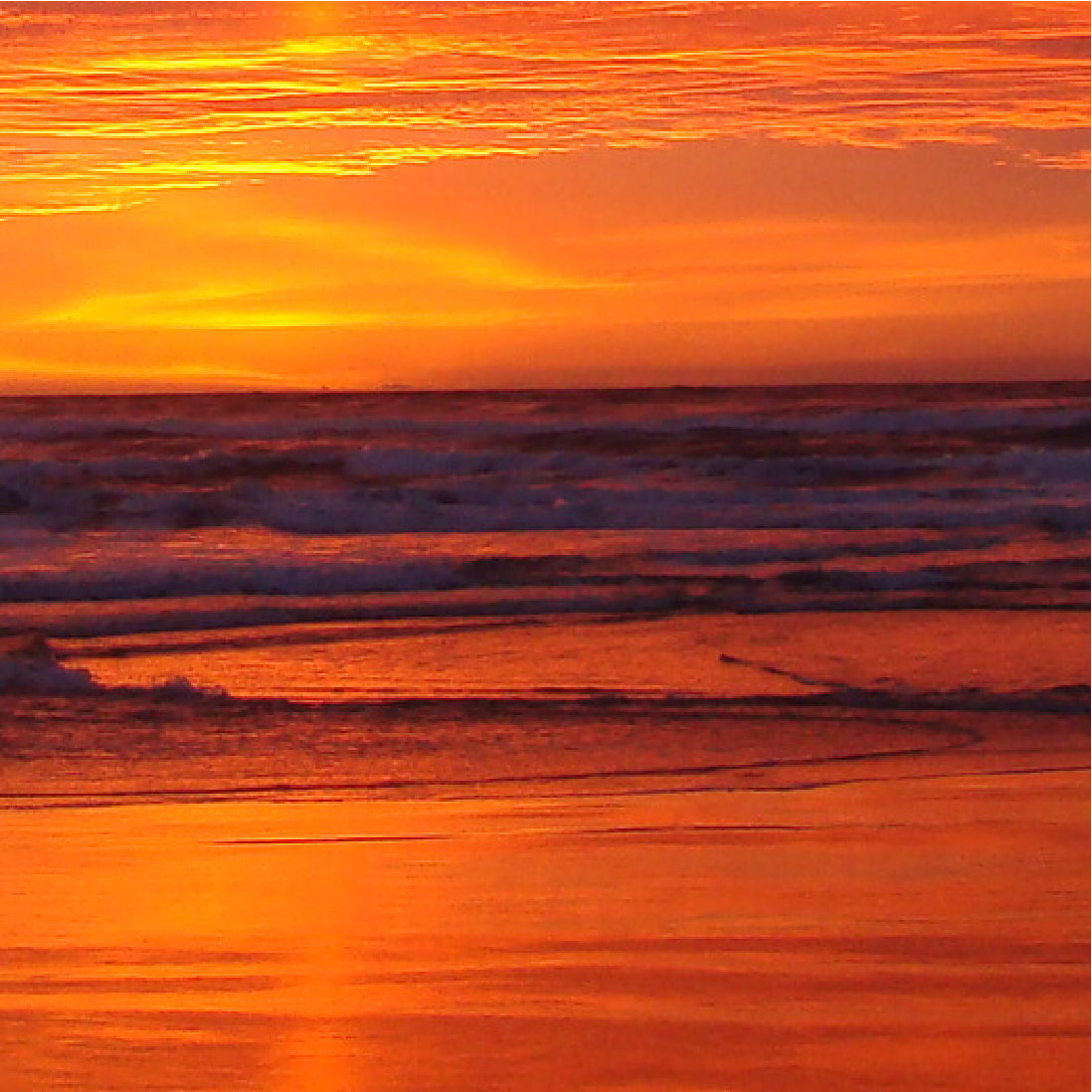 Figure 5
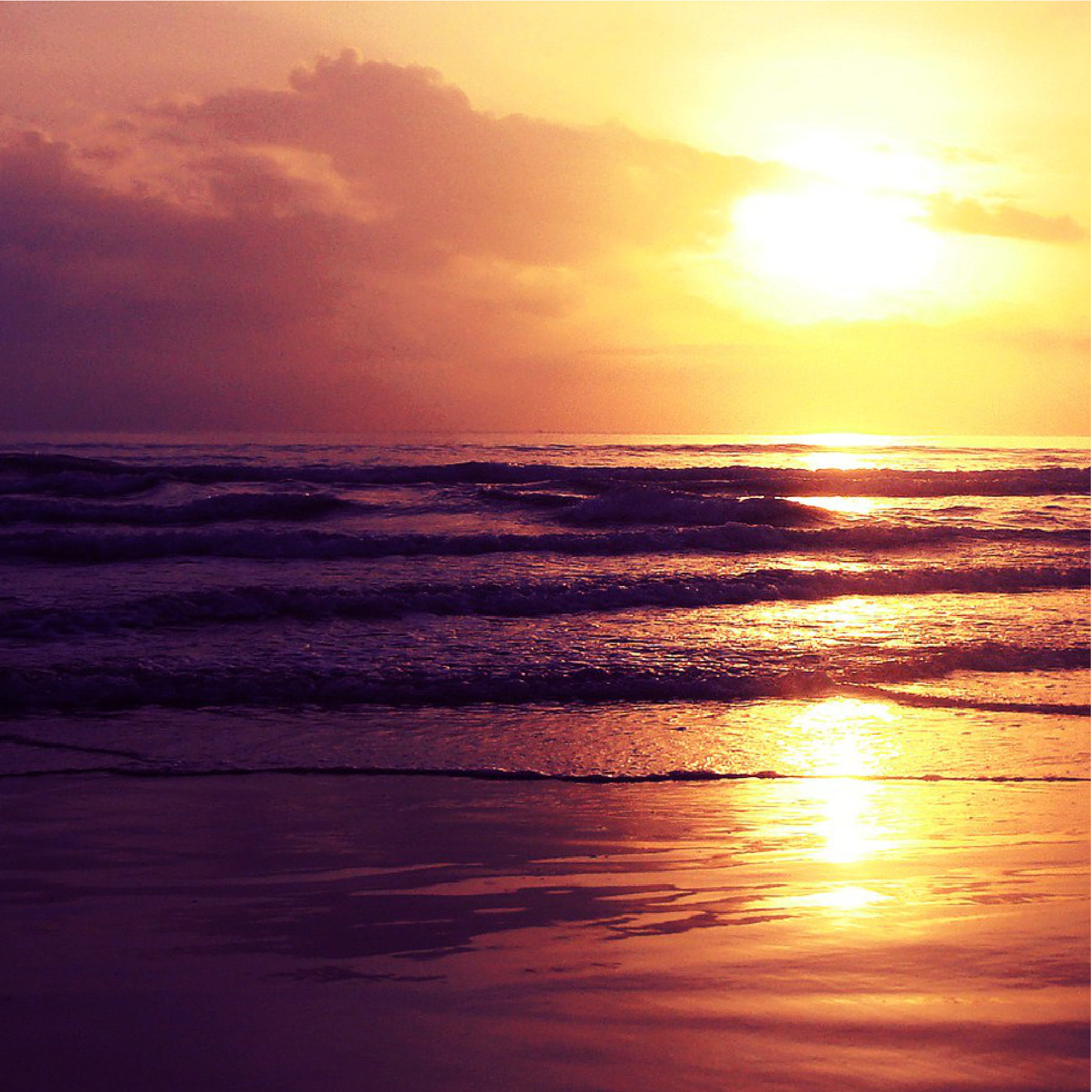 Figure 6
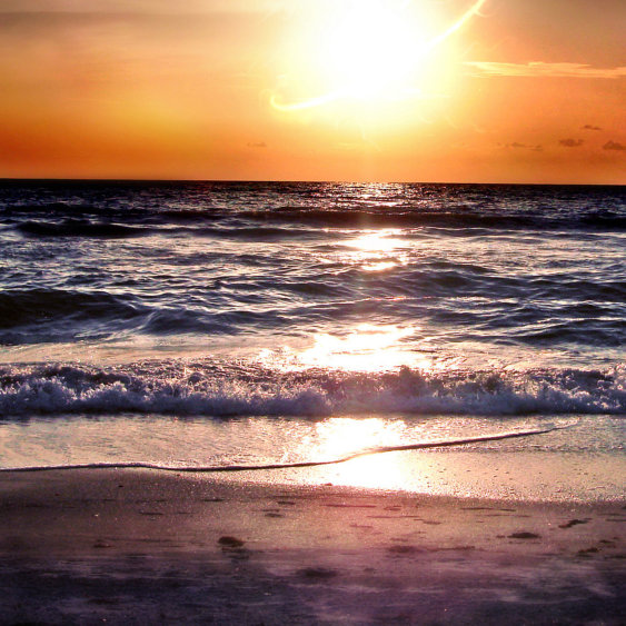 Figure 7
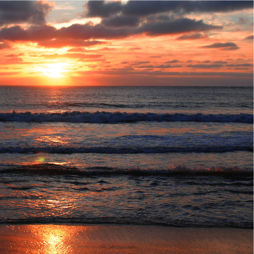 Figure 8
 Figure 9
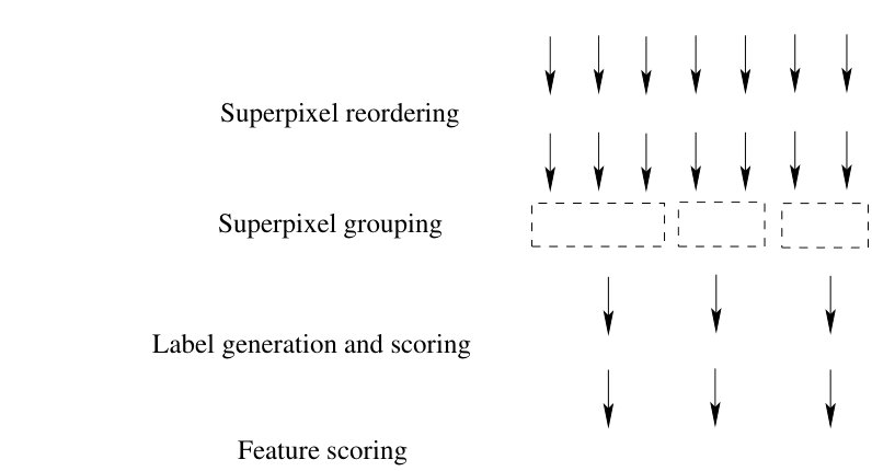 Figure 34
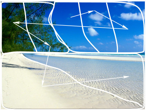 Figure 35
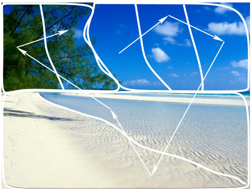 Figure 36
| Lines | Reordering + Grouping Model | Label Dependency Model | Visual Model | FAR (%) | FRR (%) | EER (%) |
|---|---|---|---|---|---|---|
| 1: | Yes/No | flat | flat | 25.00 | 75.00 | 50.00 |
| 2: | No | flat | learned | 04.98 | 28.81 | 16.90 |
| 3: | No | learned | flat | 13.47 | 41.26 | 27.36 |
| 4: | No | learned | learned | 03.11 | 11.34 | 07.22 |
| 5: | Yes + flat | flat | learned | 04.98 | 28.78 | 16.88 |
| 6: | Yes + flat | learned | flat | 11.43 | 36.52 | 23.98 |
| 7: | Yes + flat | learned | learned | 02.70 | 08.64 | 05.67 |
| 8: | Yes + learned | flat | learned | 04.98 | 28.96 | 16.97 |
| 9: | Yes + learned | learned | flat | 11.13 | 33.99 | 22.56 |
| 10: | Yes + learned | learned | learned | 02.49 | 07.80 | 05.14 |
Peer Reviews
No public reviews on file for this paper yet. If you reviewed it on a platform where reviews are public (OpenReview, ICLR, NeurIPS, ICML), you can paste yours below so the community can read it here.
Videos
No videos yet. Explain this paper in a talk, walkthrough, or lecture? Add one.
Taxonomy
TopicsAdvanced Image and Video Retrieval Techniques · Machine Learning and Algorithms · Image Retrieval and Classification Techniques
Finite State Machines for Semantic Scene Parsing and Segmentation
Hichem Sahbi
CNRS, LIP6 Lab, Sorbonne University, Paris
Abstract
We introduce in this work a novel stochastic inference process, for scene annotation and object class segmentation, based on finite state machines (FSMs). The design principle of our framework is generative and based on building, for a given scene, finite state machines that encode annotation lattices, and inference consists in finding and scoring the best configurations in these lattices. Different novel operations are defined using our FSM framework including reordering, segmentation, visual transduction, and label dependency modeling. All these operations are combined together in order to achieve annotation as well as object class segmentation.
Keywords: Finite state machines, scene parsing and segmentation
I Introduction
The general problem of image annotation is usually converted into classification. Many existing state of the art methods (see for instance [1, 2, 3, 4, 5, 6, 7, 8, 9, 10, 11, 12, 13, 14, 15, 16, 17]) treat each keyword (also referred to as label or category) as a class, and then build the corresponding category-specific classifier in order to identify images or image regions belonging to that class, using a variety of machine learning techniques such as Markov models [18, 19, 20, 21], latent Dirichlet allocation [22, 23, 24, 25], probabilistic latent semantic analysis [26, 27, 28], support vector machines [29, 30, 31, 32, 33, 34, 19, 35, 36], deep learning [37, 38, 39, 40, 41, 42, 43, 44, 45, 46], etc. Annotation methods may also be categorized into: region-based object class segmentation (OCS) requiring a preliminary step of image segmentation (e.g., [47, 48, 49, 50, 51, 52, 53, 54, 55, 56, 57, 58], etc.), and holistic (e.g., [59, 11, 60, 61, 17, 62, 63, 29, 64], etc.) operating directly on the entire image space. In both cases, training is achieved in order to learn how to attach labels to the corresponding visual features.
In this paper, we introduce an original OCS method based on FSMs. Our approach is Bayesian; it finds superpixel labels that maximize a posterior probability, but its key-novelty resides in the representational power of FSMs in order to build a comprehensive model for scene segmentation and labeling. Indeed, we translate our OCS into searching, via FSMs, the optimum of a discrete energy function mixing i) a unary term that models conditional probability of visual features given their (possible) labels, ii) an interaction potential which provides joint statistics, of co-occurrence, between those labels, and more importantly iii) a novel reordering and grouping term. The latter allows us, via FSMs, to examine (generate, label, score and rank) many partitions of segments of a scene, and to return only the likely ones.
At least two reasons drove us to apply FSMs for OCS:
i) Firstly, as FSMs can model huge (even infinite) languages111In OCS, the alphabet of the language corresponds to all the superpixels of a given scene., with finite memory and time resources, our method does not require explicit generation of all possible segmentations and labelings. Instead, it first models them implicitly by combining (composing) different FSMs and then efficiently finds the shortest path (i.e., the most likely segmentation and labeling) in a global FSM.
ii) Secondly, superpixel reordering allows us to examine the possible segmentations at different orders and, using the chain rule, to maximize the interaction potentials resulting into better labeling. For that purpose, scenes are first described with graphs where nodes correspond to superpixels and edges connect neighboring superpixels. Then, reordering is achieved by generating random (Hamiltonian) walks on these graphs using FSMs. Note that graphs with very low connectivity ( immediate neighbors for each superpixel) dramatically reduce the complexity of this reordering and also grouping while, at the same time, make it possible to explore larger sets of possible solutions resulting into an effective and also efficient scene labeling machinery as discussed later in this paper.
II Scene Labeling Model
Given lattice points , we define in this section as a set of observed random variables, corresponding to a subdivision of an image into smaller units, referred to as superpixels. Let be a random partition of ; an element is defined as a collection of conditionally independent random variables (here ) and the underlying (unknown) labels taken from a label set .
For a given observed superpixel set , our scene labeling defines a joint probability distribution over multiple superpixel reorderings, groupings (segmentations), labelings and finds the best tuple as the max of the following probability distribution
[TABLE]
Here denotes a permutation (reordering) that maps each element to and denotes the symmetric group on including all the bijections (permutations) from to it-self. The model above illustrates a generative scene labeling process which first (i) reorders (in multiple ways) the lattice resulting into , (ii) partitions/groups (in multiple ways) into subsets , then (iii) emits (in multiple ways) label hypotheses for the segments and finally (iv) estimates their visual likelihood so only relevant labels will be strengthened. Example in Fig. (1, top) illustrates one realization of this stochastic process.
Note that a naive and brute force generation of all the possible reorderings, groupings, labelings would be out of hand; as detailed in the subsequent sections, our approach does not explicitly generate all these configurations, but instead implicitly specifies them using finite state machines in order to build a scored lattice of possible segmentations and labelings.
II-A Reordering & Grouping Models for Multiple Image Segmentation
Reordering corresponds to permutations that transform an image lattice into many words in , while grouping breaks every word into subwords. Applying all the permutations , followed by all the possible groupings makes it possible to generate all the possible partitions of . Subsets in each partition (again denoted ) are defined as , with . Reordering and grouping models, also shown in Eqs. 2-3, are necessary not only to delimit segment boundaries with a high precision but also to evaluate label dependencies between segments at multiple orders (see section II-B and Fig. 1, bottom).
In this work, we restrict image partitions to include only connected segments with homogeneous superpixels. For that purpose our superpixel grouping follows random walks (RWs): it randomly visits superpixels in (graph associated to the lattice ), and groups (with a high probability) only connected and visually similar ones. Each RW corresponds to a path in which is not necessarily Hamiltonian. If one restricts RWs to include only permutations, then the resulting paths will be Hamiltonian222Note that planar 4-connected graphs (including 4-connected regular grids) are necessarily Hamiltonian. and correspond to partitions of that necessarily include connected subsets.
Considering the lattice , our reordering model equally weights permutations in , i.e., , while our grouping model assumes all segments in a given partition conditionally independent given , so one may write . All the partition sizes have the same mass, i.e., , and . Here is taken as uniform, i.e., and is taken as the random walk transition probability from node (superpixel) to node , which is positive only if the underlying superpixels share a common boundary and it is set to P(\mathbb{\pi}_{k_{i}+j}|\mathbb{\pi}_{k_{i}+j-1})\ \propto\ \mathds{1}_{\{(\mathbb{\pi}_{k_{i}+j},\mathbb{\pi}_{k_{i}+j-1})\in E\}}\cdot{\bf\kappa}\big{(}\psi(\mathbb{\pi}_{k_{i}+j}),\psi(\mathbb{\pi}_{k_{i}+j-1})\big{)}; here is the histogram intersection kernel and denotes a visual feature extracted at superpixel . With this model, if the transition between neighboring superpixels is achieved with a high conditional probability, then these superpixels are considered as visually similar and likely to come from the same physical object.
II-B Visual and Label Dependency Models
Once superpixels reordered and grouped in multiple ways, we use a unary visual and label interaction models, described below, in order to score the resulting partitions. As shown in the remainder of this paper, only highly scored partitions are likely to correspond to correct object segmentations.
Label Dependency Model. This model captures scene structure and a priori knowledge about segment/label relationships (either co-occurrence or geometric relationships) in order to consolidate labels which are consistent with already observed scenes. Considering a first order Markov process and using the chain rule, our bi-gram label dependency model is .
Let be a training set, of fixed size images, labeled at the pixel level (with labels in ). Let be the frequency of co-occurrence of pixel and label in . Similarly, we define as . Given superpixels , with labels resp. as , , we define
[TABLE]
Visual Model. This defines the likelihood of given the labels . Assuming conditionally independent superpixels and segments given their labels, and assuming that each depends only on , we define our visual model as
[TABLE]
here is an SVM classifier (based on histogram intersection kernel) trained, using LIBSVM, to discriminate superpixels belonging to a category from .
III Finite State Machine Inference
In this section, we implement the models discussed earlier using FSMs. We remind, in [65], the definition of stochastic FSMs333All the definitions and implementations of FSMs are reported in the technical report [65]., in particular finite state acceptors (FSA) and transducers (FST), and we show how we design and combine those machines in order to build a global transducer. The latter encodes in a compact way, the lattice of possible annotations of a given scene and the best annotation corresponds to the best path in that lattice.
Given a scene paved with a collection of non-overlapping superpixels, our labeling model first reorders these superpixels (via a “reordering FSA” ) and group them (via a “grouping FST” ). These two FSMs when composed together, allow us to generate many reordered partitions of segments444Each segment in these partitions is seen as a “phrase” in a “language” with an alphabet corresponding to all the superpixels of a scene.. Among these partitions, only a few of them are relevant and correspond to meaningful objects in the scene. Therefore, and in order to find these relevant partitions, we combine the and FSMs with (resulting from the composition of visual and label dependency FSTs; see example in [65]) that scores segments in all possible partitions, depending on their unary and binary interactions, and returns only the most likely partition and its labels. The most likely solution (partition and its labels) corresponds to the best (shortest) path in the global FSM () provided that negative log-likelihood transform is applied to all FSM transition probabilities; this solution also minimizes the energy (see Eq. 1). Figure 2 shows an example of this global FSM.
Note that the global composition process () could be time and memory demanding. One may significantly reduce complexity of different transducers (and thereby the global one) at different levels including the visual and the label dependency models by only keeping sparse transitions (related to strictly positive or large statistics). Another simplification consists in reducing the number of possible labels, especially if one is interested in domain specific applications with restricted labels. In practice, with these simplifications (and besides superpixel and feature extraction), FSM inference takes 2s to annotate an image of superpixels using a standard 3Ghz PC.
IV Validation and Discussion
Evaluation Set and Setting. In order to validate the proposed OCS approach, we use the “Sunset04” database. The latter contains 100 sunset scenes with objects belonging to 4 categories (“Sky”, “Sea”, “Sand” and “Sun”); note that this database is challenging and interesting for our model as it has visually confusing categories (such as “Sky vs. Sea”, etc.). Given an image, the goal is to assign each group of pixels (i.e., superpixel) to one of these 4 categories. In practice, a given image is subdivided into a regular grid of 400 () superpixels, each one is connected to its 4 immediate neighbors: top, bottom, left, right (see other e.g. [66, 67]) and described using the bag-of-word SIFT representation. Precisely, dense SIFT features are extracted and quantized using a codebook of 200 visual words and a two level spatial pyramid is used to describe each superpixel resulting into a feature vector of 1000 dimensions.
For each image in Sunset04, we turn OCS into an FSM decoding process (as described earlier); half of the Sunset04 database is used in order to train (obtain statistics of) different FSMs (i.e., label dependency and visual models) while the other half is used as a test set for OCS decoding. For each category, we measure the underlying false acceptance rates (FAR) and false rejection rates (FRR) as well as the equal error rates (as average of FAR and FRR) all at the pixel level; we report the mean accuracy as the expectation of these errors through different categories.
Model Evaluation. Table I reports the accuracy of our FSM decoding for different setting of our model. The main goal is to understand the contribution of each step in the FSM decoding/inference process. In this table, “Yes” stands for the use of the grouping+reordering models; the transition probabilities of the random walk grouping model are either uniform (flat) or set (learned) as described in Section II. A “No” stands for no-reordering which means that a given test image is parsed using a unique order (lexicographic in practice). We also consider, in these experiments, flat and learned label dependency and visual models. Flat models mean that all the underlying statistics are uniform while learned models correspond to statistics taken from Eqs. 6-7. In contrast to flat reordering+grouping models, setting flat label dependency (or visual) model is strictly equivalent to the “non-use” of that model as its impact on the decoding process becomes completely neutral.
Impact of Reordering and Grouping Model. Lines 2-4 vs. 5-10, show that the OCS performances are consistently better when using reordering (R) and grouping (G) models as the latter parse and group superpixels with different orders. This results into a better exploration of the space of possible solutions of Eq. 1 (segmentations, labelings and dependencies) and thereby a better OCS performance. Note that learned R and G models (Lines 8-10) always outperform flat ones (Lines 5-7), as the (random walk-based) grouping model gives more preference and better scoring to visually similar superpixels which are more likely to correspond to actual objects.
Impact of Dependency and Visual Models. It is interesting to see that the gain when using the visual model (without dependency model, i.e., lines 2, 5, 8) is more important than the gain obtained when using the dependency model (without visual model, i.e., lines 3, 6, 9), as the former is image/content dependent while the latter acts as a prior/context. However, it is clear that the gain obtained when combining both models is more substantial and always consistent (lines “4 vs. 2”, “7 vs. 5”, “10 vs. 8”). Note that line 1 is strictly equivalent to void dependency and visual models, and the underlying results correspond to a random classifier, that assigns random class labels to superpixels; the same behavior is observed both with and without the reordering and grouping model. This observation shows that the FSM decoding process is able to benefit from reordering and grouping only if visual and dependency models are able to score the resulting segmentation with a decent precision. The converse is also true as the effect of reordering+grouping on the decoding process is clearly important (lines 5-10 vs. 2-4; see also Fig. 3).
V Conclusion
In this paper, we introduced a complete framework for scene parsing and annotation based on finite state machines. The approach allows us to examine and score many configurations in order to achieve segmentation as well as annotation. Instead of generating intractable configurations of segmentations and labelings, the method relies on finite state machines in order to specify a lattice of these configurations and the best one (reordering, segmentation, labeling and scoring) corresponds to the shortest path in that lattice. Experiments show that indeed this method is very effective for object class segmentation.
The reference list from the paper itself. Each links out to its DOI / PubMed record.
- 1[1] G. Carneiro and N. Vasconcelos, “Formulating semantic image annotation as a supervised learning problem,” in Proc. of CVPR , 2005.
- 2[2] H. Sahbi, Coarse-to-fine support vector machines for hierarchical face detection , Ph.D. thesis, Versailles University, 2003.
- 3[3] S. Tollari, P. Mulhem, M. Ferecatu, H. Glotin, M. Detyniecki, P. Gallinari, H. Sahbi, and Z-Q. Zhao, “A comparative study of diversity methods for hybrid text and image retrieval approaches,” in Workshop of the Cross-Language Evaluation Forum for European Languages . Springer, 2008, pp. 585–592.
- 4[4] X. He, R.S. Zimel, and M.A. Carreira, “Multiscale conditional random fields for image labeling,” In CVPR , 2004.
- 5[5] A. Singhal, L. Jiebo, and Z. Weiyu, “Probabilistic spatial context models for scene content understanding,” In CVPR , 2003.
- 6[6] N. Bourdis, D. Marraud, and H. Sahbi, “Constrained optical flow for aerial image change detection,” in Geoscience and Remote Sensing Symposium (IGARSS), 2011 IEEE International . IEEE, 2011, pp. 4176–4179.
- 7[7] S. Nowak and M. Huiskes, “New strategies for image annotation: Overview of the photo annotation task at imageclef 2010,” in The Working Notes of CLEF 2010 , 2010.
- 8[8] N. Boujemaa, F. Fleuret, V. Gouet, and H. Sahbi, “Visual content extraction for automatic semantic annotation of video news,” in the proceedings of the SPIE Conference, San Jose, CA , 2004, vol. 6.