Two kinematically distinct old globular cluster populations in the Large Magellanic Cloud
Andr\'es E. Piatti, Emilio J. Alfaro, Tristan Cantat-Gaudin

TL;DR
This study uses Gaia DR2 data to identify two distinct kinematic populations of old globular clusters in the LMC, revealing differences in their motion and spatial distribution, suggesting a common formation process.
Contribution
It uncovers two kinematically distinct old globular cluster populations in the LMC using Gaia data, linking their dynamics to possible simultaneous halo and disc formation.
Findings
Two kinematic groups with different velocities and spatial distributions.
Clusters with smaller vertical velocities are part of the LMC disc.
Clusters with larger velocities form a spherical component.
Abstract
We report results of proper motions of 15 known Large Magellanic Cloud (LMC) old globular clusters (GCs) derived from the Gaia DR2 data sets. When these mean proper motions are gathered with existent radial velocity measurements to compose the GCs' velocity vectors, we found that the projection of the velocity vectors onto the LMC plane and those perpendicular to it tell us about two distinct kinematic GC populations. Such a distinction becomes clear if the GCs are split at a perpendicular velocity of 10 km/s (absolute value). The two different kinematic groups also exhibit different spatial distributions. Those with smaller vertical velocities are part of the LMC disc, while those with larger values are closely distributed like a spherical component. Since GCs in both kinematic-structural components share similar ages and metallicities, we speculate with the possibility that their…
Click any figure to enlarge with its caption.
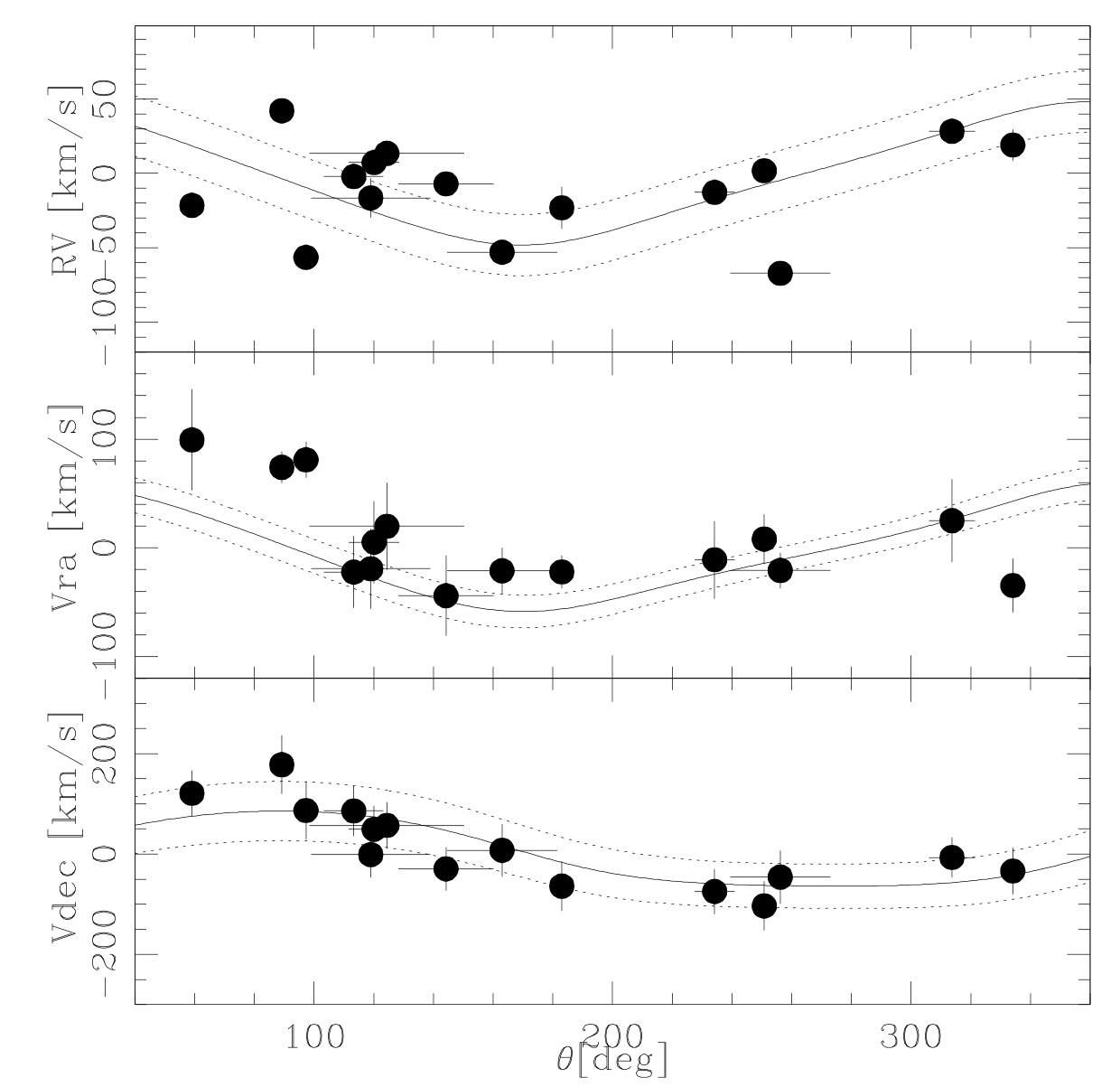 Figure 1
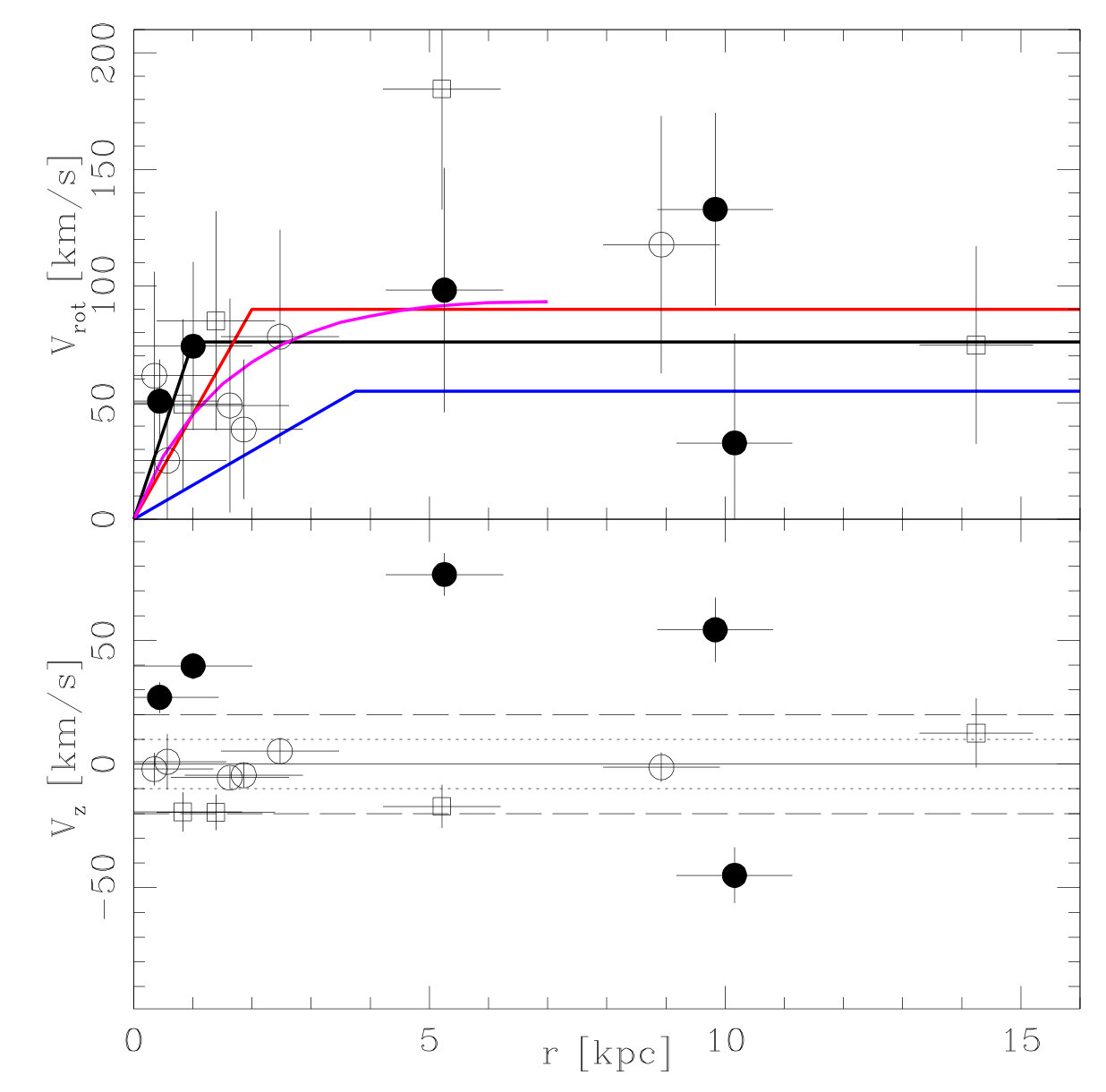 Figure 1
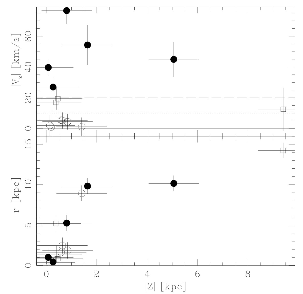 Figure 1
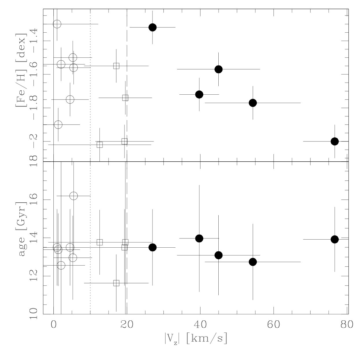 Figure 1
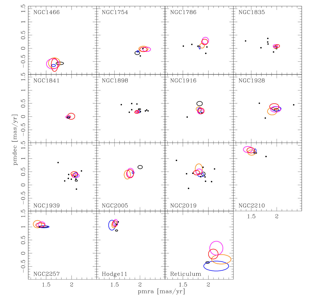 Figure 2
| ID | pmra | pmdec | n | classa | Age | [Fe/H] | ||||
|---|---|---|---|---|---|---|---|---|---|---|
| (mas/yr) | (mas/yr) | (kpc) | (kpc) | (km/s) | (km/s) | (Gyr) | (dex) | |||
| NGC 1466 | 1.7690.074 | -0.5710.050 | 8-105 | 8.92 | 1.40 | 117.855.2 | -1.25.9 | disc | 13.381.90 | -1.900.10 |
| NGC 1754 | 1.9470.048 | -0.1770.063 | 19-86 | 2.47 | 0.63 | 78.345.9 | 5.25.2 | disc | 12.962.20 | -1.500.10 |
| NGC 1786 | 1.8020.017 | 0.0770.021 | 13-207 | 1.86 | -0.84 | 38.529.9 | -4.45.1 | disc | 13.502.00 | -1.750.10 |
| NGC 1835 | 1.9940.013 | -0.0050.024 | 23-341 | 1.00 | 0.07 | 74.236.0 | 39.75.4 | halo | 13.972.80 | -1.720.10 |
| NGC 1841 | 1.9370.026 | -0.0320.031 | 6-184 | 14.25 | 9.40 | 74.742.3 | 12.514.0 | disc | 13.771.70 | -2.020.10 |
| NGC 1898 | 1.9960.017 | 0.2830.020 | 15-282 | 0.43 | 0.26 | 50.617.9 | 26.96.2 | halo | 13.502.00 | -1.320.10 |
| NGC 1916 | 1.8280.055 | 0.4940.083 | 27-165 | 0.34 | 0.13 | 61.544.5 | -2.06.5 | disc | 12.565.50 | -1.540.10 |
| NGC 1928 | 1.9910.040 | 0.2590.054 | 15-51 | 0.56 | 0.19 | 25.129.7 | 0.911.2 | disc | 13.502.00 | -1.300.10 |
| NGC 1939 | 2.0920.023 | 0.1630.028 | 6-197 | 0.83 | 0.45 | 49.336.3 | -19.37.9 | disc | 13.502.00 | -2.000.10 |
| NGC 2005 | 2.0030.044 | 0.6760.063 | 22-99 | 1.39 | 0.40 | 85.047.0 | -19.57.2 | disc | 13.774.90 | -1.740.10 |
| NGC 2019 | 1.9030.034 | 0.4130.075 | 10-262 | 1.62 | 0.58 | 48.845.8 | -5.44.6 | disc | 16.203.10 | -1.560.10 |
| NGC 2210 | 1.5780.030 | 1.2120.025 | 7-139 | 5.21 | 0.38 | 184.651.7 | -17.08.8 | disc | 11.631.50 | -1.550.10 |
| NGC 2257 | 1.4480.090 | 1.0120.028 | 10-122 | 9.83 | -1.63 | 132.941.3 | 54.313.0 | halo | 12.742.00 | -1.770.10 |
| Hodge 11 | 1.5410.023 | 0.8610.028 | 7-200 | 5.25 | 0.80 | 98.252.4 | 76.68.6 | halo | 13.921.70 | -2.000.10 |
| Reticulum | 1.9840.035 | -0.3500.035 | 7-98 | 10.16 | -5.05 | 32.747.0 | -44.911.3 | halo | 13.092.10 | -1.570.10 |
Peer Reviews
No public reviews on file for this paper yet. If you reviewed it on a platform where reviews are public (OpenReview, ICLR, NeurIPS, ICML), you can paste yours below so the community can read it here.
Videos
No videos yet. Explain this paper in a talk, walkthrough, or lecture? Add one.
Two kinematically distinct old globular cluster
populations in the Large Magellanic Cloud
Andrés E. Piatti1,2, Emilio J. Alfaro3, Tristan Cantat-Gaudin4
1Consejo Nacional de Investigaciones Científicas y Técnicas, Godoy Cruz 2290, C1425FQB, Buenos Aires, Argentina
2Observatorio Astronómico de Córdoba, Laprida 854, 5000, Córdoba, Argentina
3Instituto de Astrofísica de Andalucía, (CSIC), Glorieta de la Astronomía, S/N, Granada, 18008, Spain
4Institut de Ciències del Cosmos, Universitat de Barcelona (IEEC-UB), Martí i Franquès 1, E-08028 Barcelona, Spain E-mail: [email protected]
(Accepted XXX. Received YYY; in original form ZZZ)
Abstract
We report results of proper motions of 15 known Large Magellanic Cloud (LMC) old globular clusters (GCs) derived from the Gaia DR2 data sets. When these mean proper motions are gathered with existent radial velocity measurements to compose the GCs’ velocity vectors, we found that the projection of the velocity vectors onto the LMC plane and those perpendicular to it tell us about two distinct kinematic GC populations. Such a distinction becomes clear if the GCs are split at a perpendicular velocity of 10 km/s (absolute value). The two different kinematic groups also exhibit different spatial distributions. Those with smaller vertical velocities are part of the LMC disc, while those with larger values are closely distributed like a spherical component. Since GCs in both kinematic-structural components share similar ages and metallicities, we speculate with the possibility that their origins could have occurred through a fast collapse that formed halo and disc concurrently.
keywords:
galaxies: individual: LMC – galaxies: star clusters: general
††pubyear: 2018††pagerange: Two kinematically distinct old globular cluster populations in the Large Magellanic Cloud–Two kinematically distinct old globular cluster populations in the Large Magellanic Cloud
1 Introduction
The orbital motions of the old globular clusters (GCs) in the Large Magellanic Cloud (LMC) have been described from radial velocity (RV) measurements by a disc-like rotation with no GCs appearing to have halo kinematics (Schommer et al., 1992; Grocholski et al., 2006; Sharma et al., 2010), so that it is expected that they do not cross the LMC disc. However, a closer look to the RV versus position angle (PA) diagram, tells us that although a general trend following the LMC disc rotation is visible, there are also some GCs that clearly depart from that relationship. This behaviour can be seen in the top-left panel of Fig. 1, built from RVs and PAs taken from Piatti et al. (2018). The curve for a LMC disc, rotating according to the solution found from proper motion measurements in 22 fields (van der Marel & Kallivayalil, 2014), is also depicted with a solid line. The dotted lines represent the curves considering the quoted errors in all the parameters involved (e.g., inclination of the disc, PA of the line-of-nodes, LMC dynamical centre, disc rotation velocity, etc) and the velocity dispersion, added in quadrature.
This observational evidence, together with some speculations about their origins (e.g. Brocato et al., 1996; Piatti & Geisler, 2013), their different kinematics with respect to the LMC halo field stars (Bekki, 2007, and references therein), the effects on their motions because of the interaction of the LMC with the Milky Way (Bekki, 2011; Carpintero et al., 2013), among others, points to the need of deriving their space velocities, so that a three-dimensional picture of their movements can be analysed. In order to obtain them, accurate proper motions are necessary. With the second data release (DR2) of Gaia mission (Gaia Collaboration et al., 2016, 2018a), this challenging goal has became to be possible for the first time. Precisely, we derive here such LMC GCs’ proper motions and from information gathered from the literature constructed their space velocity vectors. By analysing their rotational and vertical velocities, along with their relationships with the GCs’ positions in the galaxy, their ages and metallicities, we found that two groups of GCs is possible to be differentiated from a kinematics point of view.
The Letter is organised as follows: in Section 2 we describe the selection of the Gaia DR2 extracted data and the estimation of the GCs’ mean proper motions. In Section 3 we perform a rigorous transformation of RVs and proper motions in terms of the rotation in and perpendicular to the LMC plane and discuss the results to the light of possible GC formation scenarious.
2 LMC GCs’ proper motions
From the Gaia archive111http://gea.esac.esa.int/archive/, we extracted parallaxes () and proper motions in Right Ascension (pmra) and Declination (pmdec) for stars located within 10 arcmin from the centres of 15 known LMC GCs (see Table 1). We limited our sample to stars with proper motion errors 0.5 mas/yr, which correspond to 19.0 mag (Gaia Collaboration et al., 2018b). Excess noise (epsi) and significance of excess of noise (sepsi) in Gaia DR2 (Lindegren et al., 2018) were used to prune the data. D(=sepsi) 2 and epsi 1 define a good balance between data quality and number of retained objects for our sample (see also Ripepi et al., 2018). This means that we dealt with cluster red giant stars placed above the GCs’ horizontal branches. To select cluster stars we constrained our sample to those satisfying the following criteria: i) stars located at the LMC distance, i.e., 3 (see Vasiliev, 2018); ii) stars located within the tidal cluster radii taken from Piatti & Mackey (2018).
We then performed a maximum likelihood statistics (Pryor & Meylan, 1993; Walker et al., 2006) in order to estimate the mean proper motions and dispersion for different subsets of stars, namely, those with (pmra)=(pmdec) 0.1, 0.2, 0.3, 0.4 and 0.5 mas/yr, respectively. We optimised the probability that a given ensemble of stars with proper motions pmi and errors are drawn from a population with mean proper motion pm and dispersion W, as follows:
where the errors on the mean and dispersion were computed from the respective covariance matrices. We applied the above procerure for pmra and pmdec, separately.
Fig. 2 depicts the results represented by ellipses centred on the mean values and with axes equal to the derived errors. As can be seen, the larger the individual proper motion errors, the larger the derived errors of the mean proper motions, with some exception. With the aim of assuring accuracy, we constrained the subsequent analysis to the GC mean proper motions derived from stars with proper motion errors 0.1 mas/yr (see Table 1, where n refers to the number of stars used between those with proper motion errors 0.1 and 0.5 mas/yr, respectively). In order to illustrate the contamination of field stars in the GC mean proper motion estimates, we have included with black thick dots every individual field stars with proper motion errors 0.1 mas/yr lying in the sky within a circle equivalent to the size of the cluster’s circle, which is centred at 5 cluster radii away from the cluster centre. As far as we are aware, the resultant mean LMC GC proper motions represent those based on accurate measurements of bonafide cluster members.
These proper motions can be compared with those of the LMC disc by adopting the transformation equations (9), (13) and (21) in van der Marel et al. (2002) and the best-fit solutions for the rotation of the LMC disc obtained from proper motions of field stars (column 3 of Table 1 in van der Marel & Kallivayalil, 2014). We then subtracted the corresponding amount of motion of the LMC centre of mass from the GCs’ proper motions. The top-left panel of Fig. 1 shows the results as a function of the PA. As a matter of units, we used [km/s] = 4.7403885* [mas/yr], where is the distance to the LMC centre of mass (= 50.1 kpc van der Marel & Kallivayalil, 2014), and denoted Vra and Vdec the movements in R.A and Dec., respectively. We have overplotted the rotation of the LMC disc with a solid line and those considering the errors in the inclination of the disc, the PA of the line-of-nodes, the systemic and transversal velocities of the LMC centre of mass and disc velocity dispersion with dotted lines, respectively. The errorbars of the plotted GCs’ proper motions account not only for the measured errors listed in Table 1, but also for those from the adopted van der Marel & Kallivayalil (2014)’s best-fit solution for the 3D movement of the LMC centre of mass, propagated through the transformation equations and added in quadrature. As can be seen, the GC motions relative to the LMC centre projected onto the sky resemble that of the rotation of a disc, with some noticeable scatter and some GCs placed beyond that rotational pattern.
3 Analysis and discussion
The projection of the GC velocity vectors onto the LMC plane and that perpendicular to it provide us with a valuable tool to address the issue of the genuine rotation of them in the LMC disc and the orientation of their orbits around the LMC centre. In order to convert the vector (RV,Vra,Vdec) into that with components and in the LMC plane and perpendicular to it, according to the reference system defined by van der Marel et al. (2002, see their Figure 3), we inverted the matrix A = B C, where B is the matrix :
[TABLE]
with , , and being the coefficients of the transformation equation (9) and C the matrix defined in equation (5) of van der Marel et al. (2002), respectively, so that:
[TABLE]
Hence, = ( + )1/2, while the errors (), () and () were computing from propagation of errors of eq. (2). The resulting values for and are listed in Table 1.
The top-right panel of Fig. 1 shows the resulting relationships of and as a function of the deprojected distances (). At first glance, inner GCs ( 5 kpc) seem to have values in better agreement with the rotation curve of the LMC disc than those in the outer regions. However, by inspecting the versus diagram, it is possible to distinguish two groups of GCs: one group with an average velocity dispersion perpendicular to the LMC plane close to zero, and another group with 10 km/s (another plausible cut could be at 20 km/s). For the sake of the reader, we have drawn GCs with smaller than 10 km/s, between 10 and 20 km/s and larger than 20 km/s with open circles and boxes and filled circles, respectively, and traced those limits with dotted and dashed lines. Notice that, The LMC rotation curve derived from old field stars (blue line) by van der Marel & Kallivayalil (2014) does not particularly agree with GCs. Other curves (e.g. black, red, magenta lines) seem to agree better with GCs across the range of . GCs with a relatively high velocity are those that globally more depart from the LMC rotation curve. For instance, the mean difference (absolute value) between the GC values and those for the same values along the mean LMC disc rotation curve (magenta line) turned out to be 13.416.1, 24.821.1 and 28.313.0 for GCs with 10 km/s, 10 km/s Vz 20 km/s and 20 km/s (31.712.1 for 10 km/s and 18.812.6 for 20 km/s), respectively. If we consider only GCs with 5 kpc, we get 14.516.2, 15.528.6 and 30.015.3 (26.713.5 for 10 km/s and 14.714.2 for 20 km/s), respectively.
Such a kinematic distinction has also its counterpart in the spatial distribution of the GCs. The bottom-left panel shows that the farther a GC from the LMC centre, the larger its height out of the plane. Along this trend, the GCs with 10 km/s are those confined to the LMC disc, with the sole exception of NGC 1466 (=8.92 kpc). This appears to be a peculiar GC, because it has a relatively large , even though its is smaller than 10 km/s. If we considered GCs with 20 km/s, the trend would remain with the additional exception of NGC 1841 (=9.40 kpc). GCs with 10km/s expand the range 0 - 3 kpc (0 - 9 kpc if NGC 1466 is included), those with 20 km/s expand the range 0 - 5 kpc (0 - 15 kpc if NGC 1481 is included), while those with 20 km/s reached 10 kpc. As the height out of the LMC plane is considered, GCs with values smaller and larger than 10 km/s are located at values smaller than 0.5 kpc (1.5 kpc if NGC 1466 is included) and 8.6 kpc, respectively. Z values were calculated from eq. (7) in van der Marel & Cioni (2001), with distances taken from Wagner-Kaiser et al. (2017) and Piatti & Mackey (2018), and assuming distance errors of 2 kpc, i.e. twice as big the dispersion of the GCs’ distances obtained by Wagner-Kaiser et al. (2017). Both spatial regimes tell us also about two different spatial patterns, one closely related to a disc component and another more similar to an spherical one. Bekki (2007) performed numerical simulations of the LMC formation with the aim of looking for an answer to the, until then, kinematic difference between LMC halo field stars and GCs. Surprisingly, he found that GCs have little rotation and spatial distribution and kinematics similar to those of the halo stars. Our analysis, based on the velocity vectors of GCs with high agree very well with that theoretical result.
Finally, we analysed whether there is any link of these two phase-space GC populations with their ages and metallicities, so that some clues about their origins can be inferred. The analysis includes the two cuts. The bottom-right panel of Fig. 1 shows the resultant behaviours, where ages and metallicities were taken from Piatti & Mackey (2018) and Piatti et al. (2018) (see Table 1). From a maximum likelihood analysis we found that these groups of GCs are coeval at a level of 0.4 Gyr and that they hardly differ in metallicity. This means that both GC components have formed nearly at the same time, within 3 Gyr of their formation (12 age (Gyr) 14, Piatti et al., 2009; Wagner-Kaiser et al., 2018) and under similar chemical enrichment processes (the three groups expand similar [Fe/H] ranges). Because of these similarities in age and metallicity and the noticeable difference in their spatial distributions (thin disc and extended halo), we speculate with the possibility that their origins could have occurred through a fast collapse that formed halo and disc concurrently. The inner GCs with 10 km/s have remained rotating in the LMC disc since their in-situ formation. As for the formation of the GCs with higher values, they could have occurred in-situ in the LMC halo and/or stripped from the Small Magellanic Cloud (SMC), where GCs with similar ages and metallicities should have formed. As suggested by Carpintero et al. (2013), this could be a plausible explanation for the lack of old metal-poor GCs in the SMC. As for the time of the GC stripping, we do not have any hint: it could have happened at the early formation of both galaxies or during a later approach of the SMC by the LMC.
Acknowledgements
We thank the referee for the thorough reading of the manuscript and timely suggestions to improve it. We thanks Eugene Vasiliev his valuable comments on a draft version of this work. EJA acknowledges financial support from MINECO (Spain) through grant AYA2016-75931-C2-1-P. This work has made use of data from the European Space Agency (ESA) mission Gaia (https://www.cosmos.esa.int/gaia), processed by the Gaia Data Processing and Analysis Consortium (DPAC, https://www.cosmos.esa.int/web/gaia/dpac/consortium). Funding for the DPAC has been provided by national institutions, in particular the institutions participating in the Gaia Multilateral Agreement.
The reference list from the paper itself. Each links out to its DOI / PubMed record.
- 1Bekki (2007) Bekki K., 2007, MNRAS , 380, 1669 · doi ↗
- 2Bekki (2011) Bekki K., 2011, MNRAS , 416, 2359 · doi ↗
- 3Brocato et al. (1996) Brocato E., Castellani V., Ferraro F. R., Piersimoni A. M., Testa V., 1996, MNRAS , 282, 614 · doi ↗
- 4Carpintero et al. (2013) Carpintero D. D., Gómez F. A., Piatti A. E., 2013, MNRAS , 435, L 63 · doi ↗
- 5Gaia Collaboration et al. (2016) Gaia Collaboration et al., 2016, A&A , 595, A 1 · doi ↗
- 6Gaia Collaboration et al. (2018 a) Gaia Collaboration et al., 2018 a, A&A , 616, A 1 · doi ↗
- 7Gaia Collaboration et al. (2018 b) Gaia Collaboration et al., 2018 b, A&A , 616, A 12 · doi ↗
- 8Grocholski et al. (2006) Grocholski A. J., Cole A. A., Sarajedini A., Geisler D., Smith V. V., 2006, AJ , 132, 1630 · doi ↗