Optimal approximation of stochastic integrals in analytic noise model
Andrzej Ka{\l}u\.za, Pawe{\l} M. Morkisz, Pawe{\l} Przyby{\l}owicz

TL;DR
This paper investigates the optimal approximation of stochastic Itô integrals under an analytic noise model, establishing error bounds for noisy evaluations and demonstrating the impact of low-precision computations on accuracy and performance.
Contribution
It introduces a new analytic noise model for stochastic integration and derives error bounds for approximation algorithms considering low-precision evaluations.
Findings
Error bounds are proportional to $n^{- ho} + ext{precision parameters}$.
Any algorithm with at most $n$ evaluations has a lower bound error of $C(n^{- ho} + ext{precision})$.
Numerical experiments confirm theoretical error bounds and compare CPU and GPU performance.
Abstract
We study approximate stochastic It\^o integration of processes belonging to a class of progressively measurable stochastic processes that are H\"older continuous in the th mean. Inspired by increasingly popularity of computations with low precision (used on Graphics Processing Units -- GPUs and standard Computer Processing Units -- CPU for significant speedup), we introduce a suitable analytic noise model of standard noisy information about and . In this model we show that the upper bounds on the error of the Riemann-Maruyama quadrature are proportional to , where is a number of noisy evaluations of and , is a H\"older exponent of , and are precision parameters for values of and , respectively. Moreover, we show that the error of any algorithm based on at most noisy…
Click any figure to enlarge with its caption.
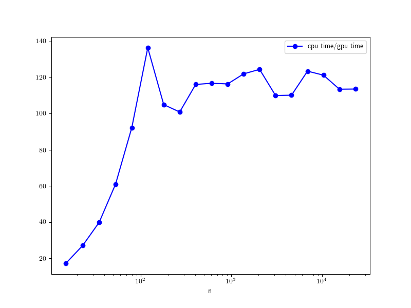 Figure 1
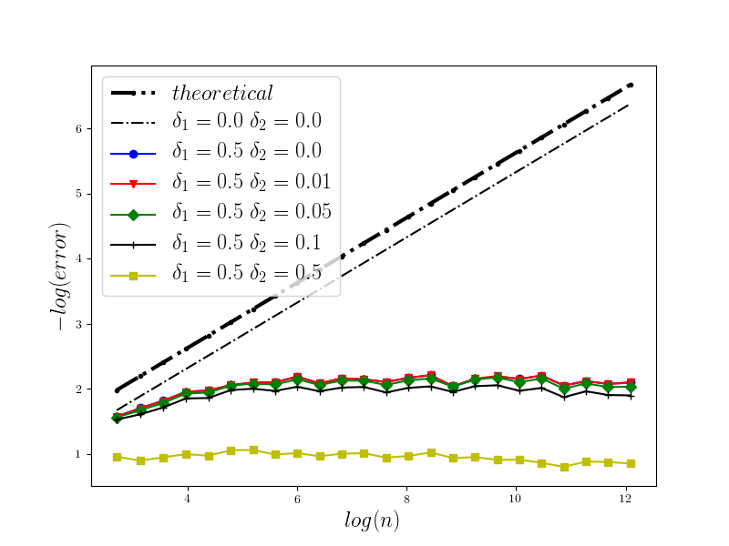 Figure 2
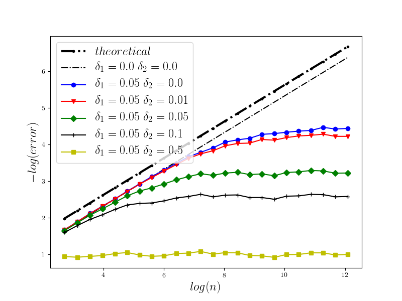 Figure 3
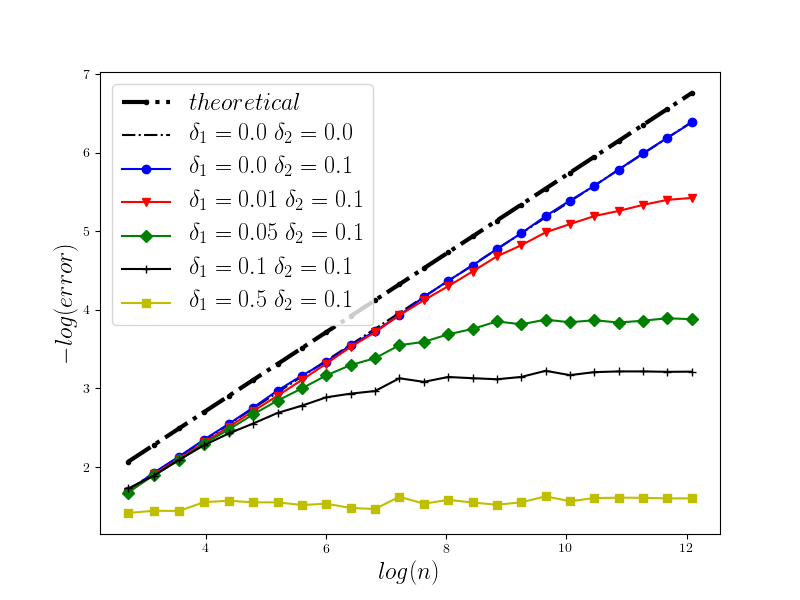 Figure 4
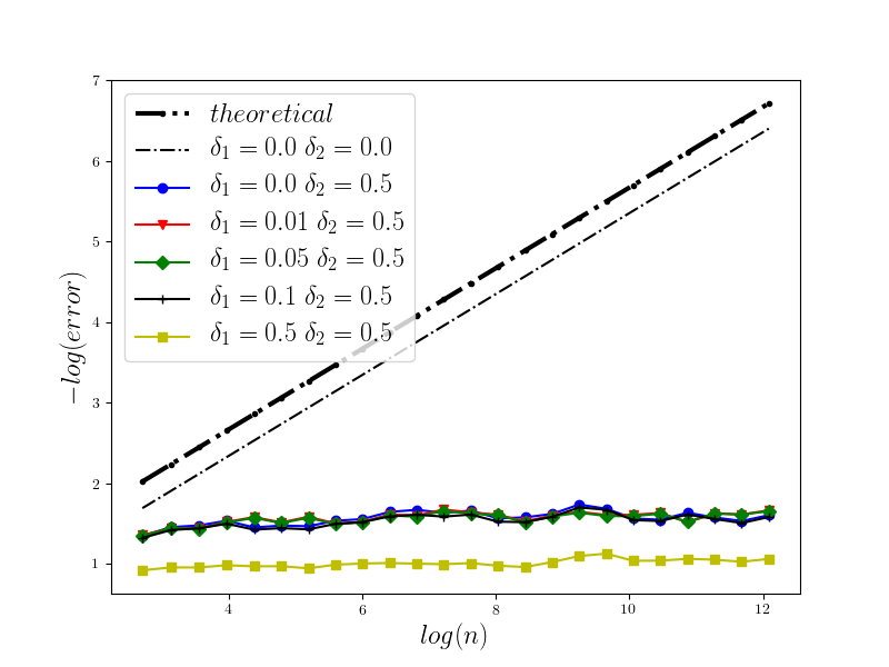 Figure 5
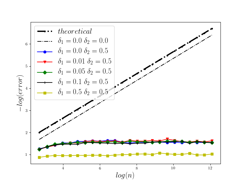 Figure 6
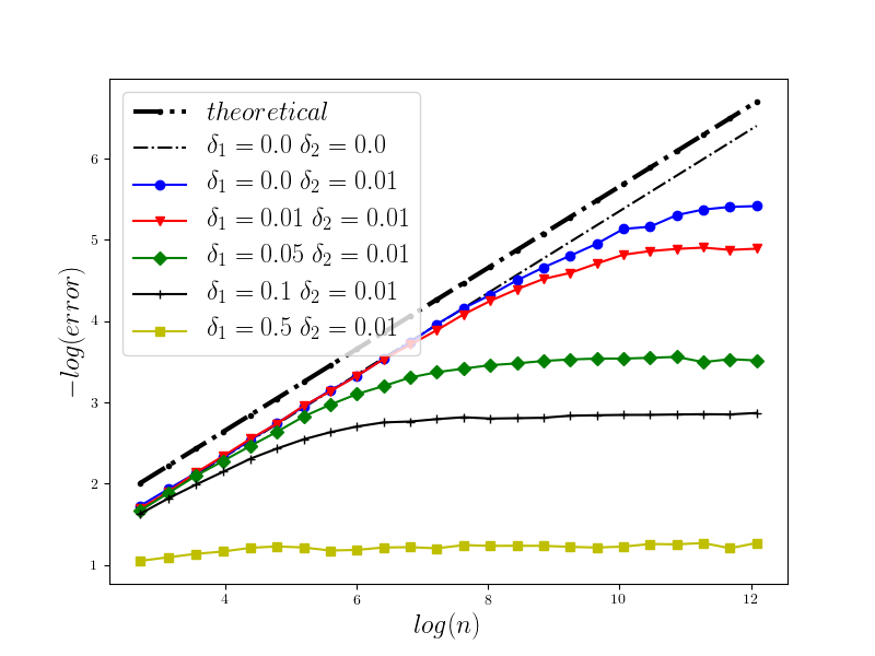 Figure 7
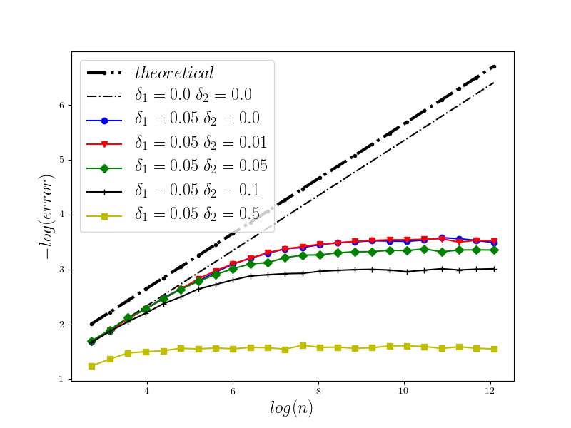 Figure 8
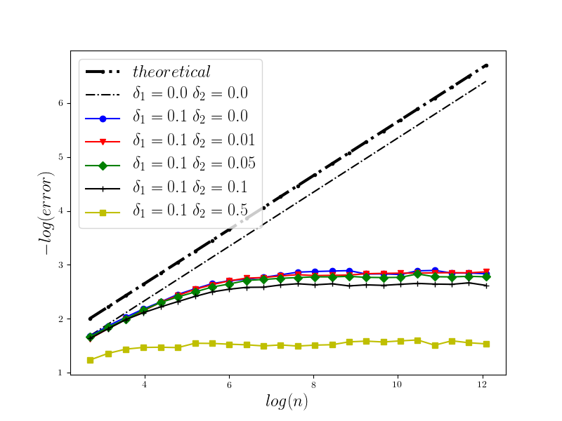 Figure 9
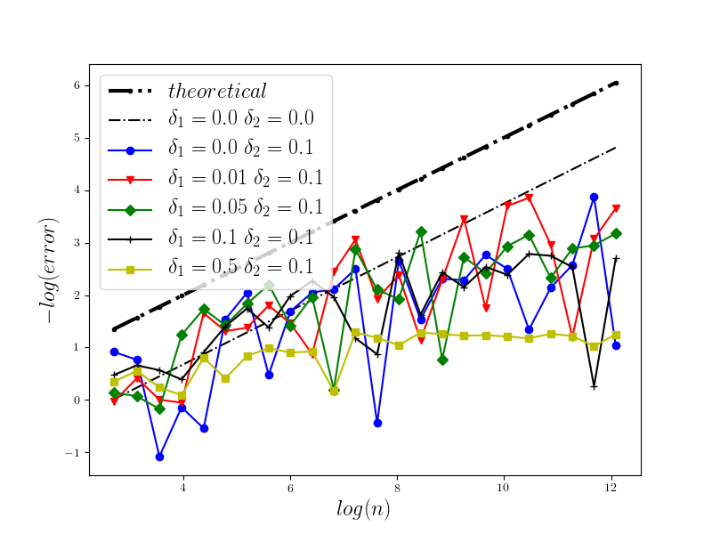 Figure 10
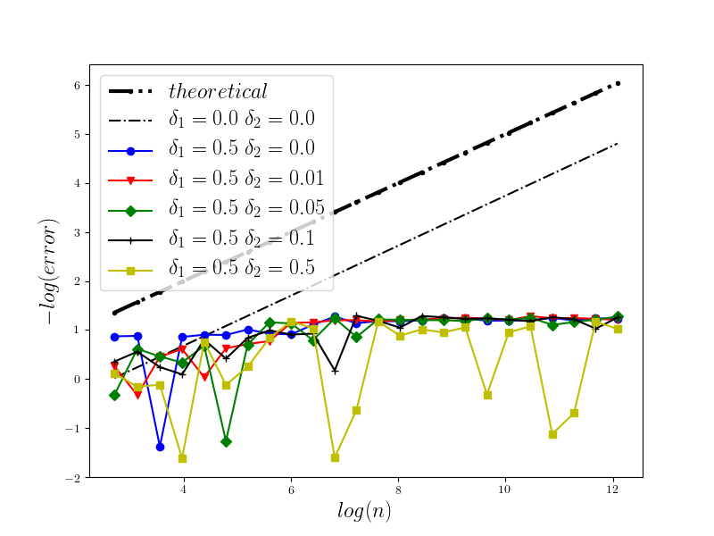 Figure 11
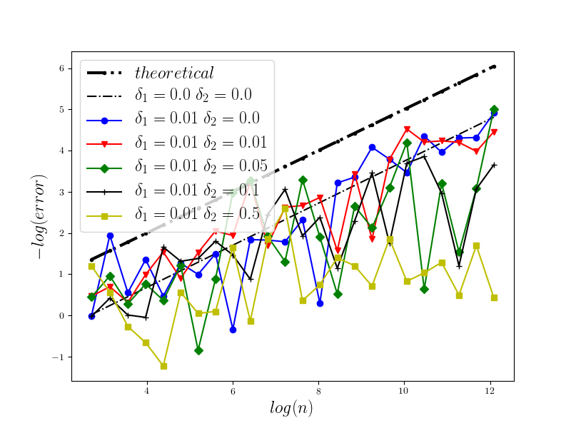 Figure 12
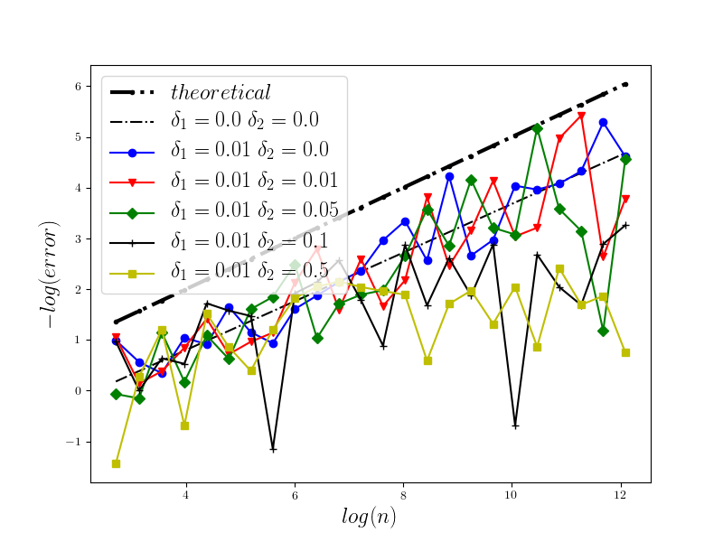 Figure 13
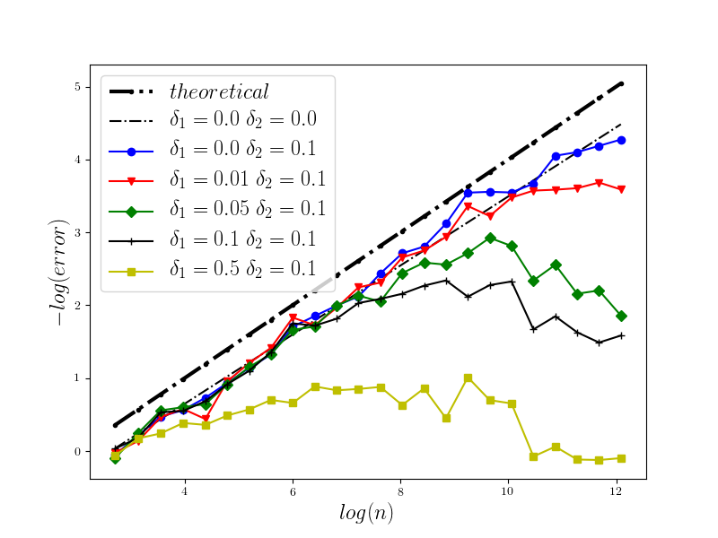 Figure 14
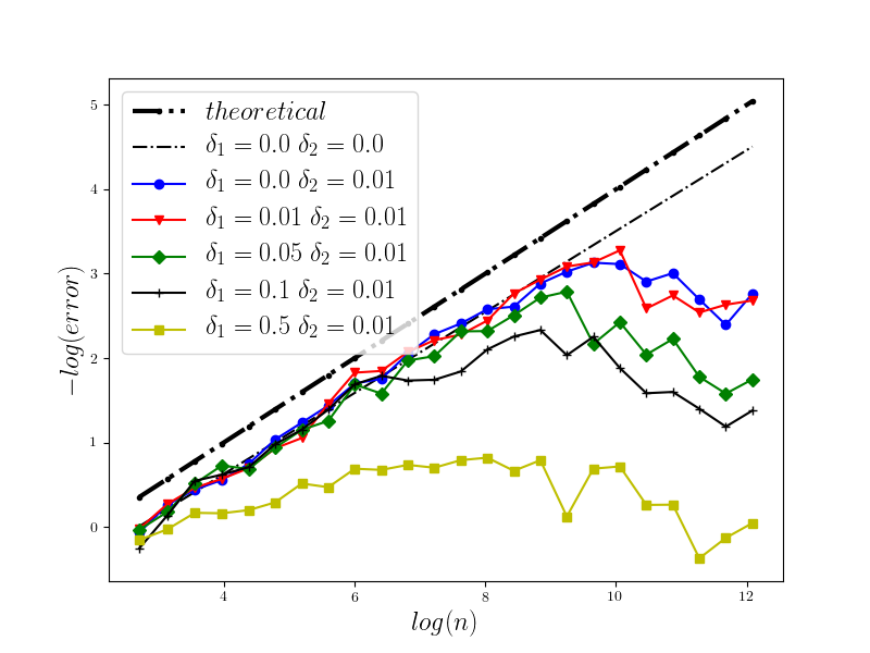 Figure 15
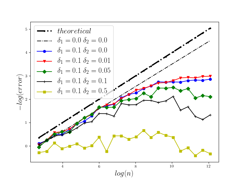 Figure 16
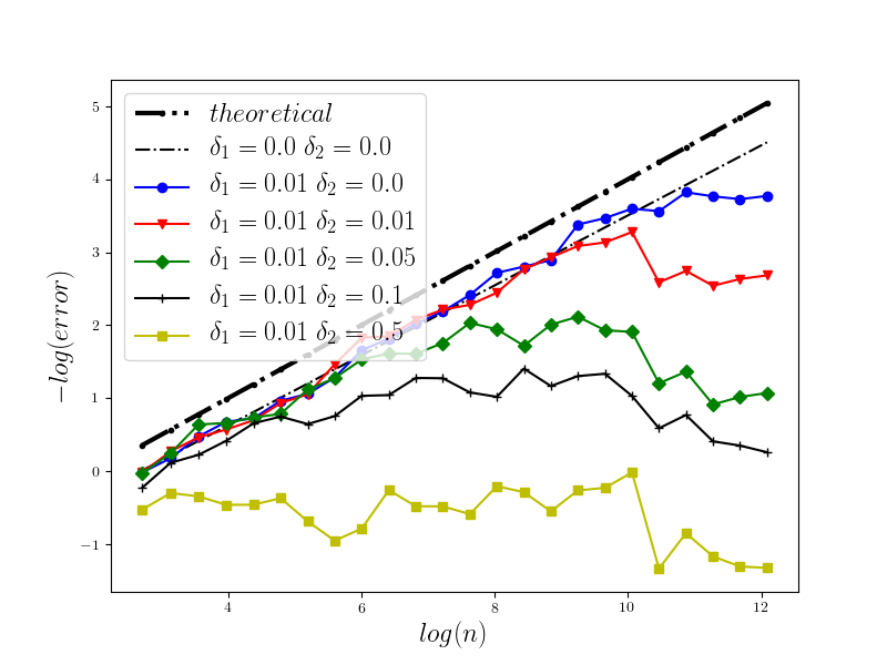 Figure 17
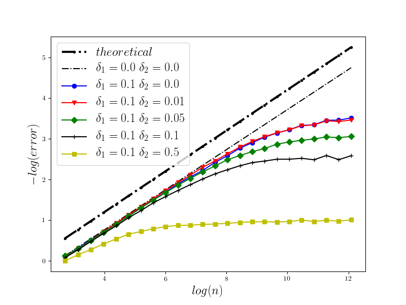 Figure 18
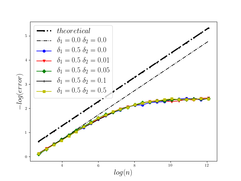 Figure 19
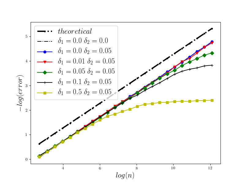 Figure 20
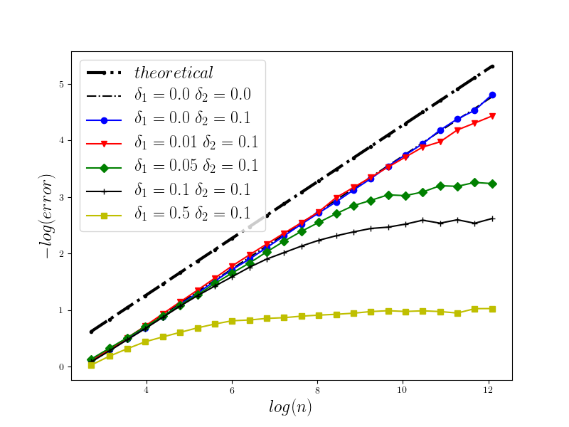 Figure 21
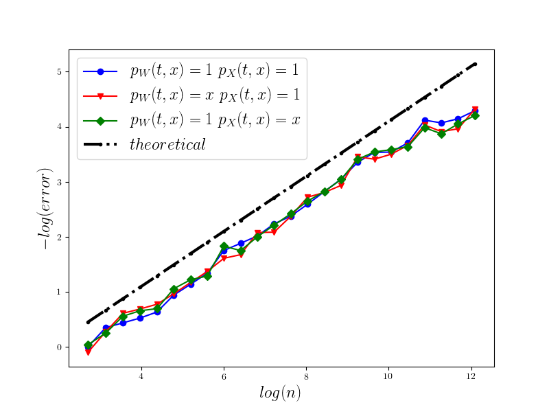 Figure 22
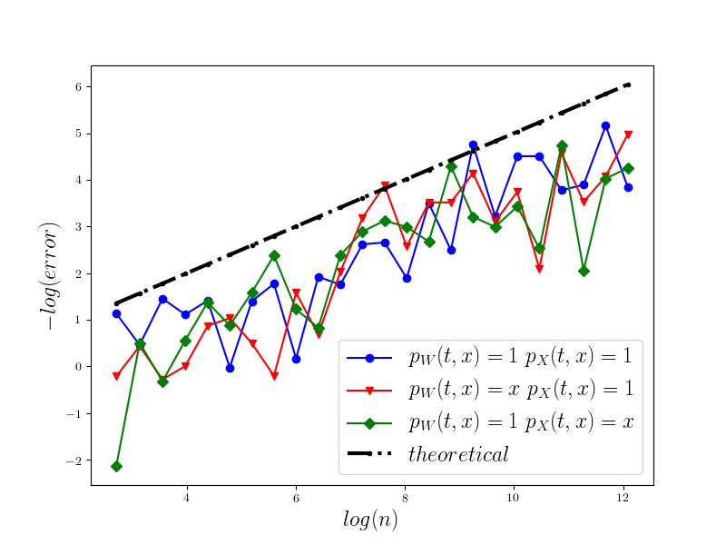 Figure 23
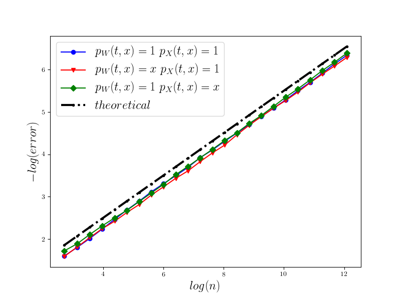 Figure 24
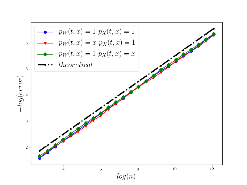 Figure 25
Peer Reviews
No public reviews on file for this paper yet. If you reviewed it on a platform where reviews are public (OpenReview, ICLR, NeurIPS, ICML), you can paste yours below so the community can read it here.
Videos
No videos yet. Explain this paper in a talk, walkthrough, or lecture? Add one.
Optimal approximation of stochastic integrals in analytic noise model
Andrzej Kałuża
AGH University of Science and Technology, Faculty of Applied Mathematics, Al. A. Mickiewicza 30, 30-059 Kraków, Poland
,
Paweł M. Morkisz
AGH University of Science and Technology, Faculty of Applied Mathematics, Al. A. Mickiewicza 30, 30-059 Kraków, Poland
and
Paweł Przybyłowicz
AGH University of Science and Technology, Faculty of Applied Mathematics, Al. A. Mickiewicza 30, 30-059 Kraków, Poland
[email protected], corresponding author
Abstract.
We study approximate stochastic Itô integration of processes belonging to a class of progressively measurable stochastic processes that are Hölder continuous in the th mean.
Inspired by increasingly popularity of computations with low precision (used on Graphics Processing Units – GPUs and standard Computer Processing Units – CPU for significant speedup), we introduce a suitable analytic noise model of standard noisy information about and . In this model we show that the upper bounds on the error of the Riemann-Maruyama quadrature are proportional to , where is a number of noisy evaluations of and , is a Hölder exponent of , and are precision parameters for values of and , respectively. Moreover, we show that the error of any algorithm based on at most noisy evaluations of and is at least . Finally, we report numerical experiments performed on both CPU and GPU, that confirm our theoretical findings, together with some computational performance comparison between those two architectures.
Key words: Wiener process, noisy information, analytic noise model, optimal approximation, minimal error, GPU
Mathematics Subject Classification: 68Q25, 65C30.
1. Introduction
In this paper we investigate the problem of optimal approximation of stochastic integrals of the following form
[TABLE]
where and is a one-dimensional Wiener process on some probability space , and we consider integrands from a class of progressively measurable stochastic processes that are Hölder continuous in the th mean. Such quadrature problems arise, for example, in the context of numerical solutions of stochastic differential equations, see Section 4.4 in [13] and [2]. Since the exact values of such stochastic integrals are known only in limited cases, an efficient approximation of with the error as small as possible is of interest. We are aiming at methods that are based only on discrete values of and which are, additionally, corrupted with some noise.
The problem of optimal approximation of stochastic Itô integrals under exact information about and has been well studied in the literature, see, [6], [7], [8], [21], [22], [23], [28]. Less explored is the approximation of stochastic integrals in the case when values of and are corrupted with some noise. The noise may arise from measurement errors, previous computations or simply the floating point numbers representation errors. There is a trend observed in deep learning, where the computations are mostly conducted in lower precision, i.e. using not only single but also half precision. Exemplary performance for NVIDIA V100 graphic card is about 7 TFLOPS for double precision and 14 TFLOPS for single precision. For deep learning purposes, using the nature of the operations and also further lowering the precision to half precision in chosen operations, enabled obtaining up to 112 TFLOPS of performance [16]. Hence, it is a huge motivation for analyzing how lowering the precision for other than deep learning applications, influence the computed result.
There are many results on solving problems under noisy information, including the problems such as integrating or approximating regular functions (see, e.g., [9, 19, 10]), approximation of piecewise regular functions (see [17]), approximate solving of IVPs (see [11]) or PDEs (see [29, 30]).
In this paper we study noisy information for stochastic Itô integration. According to our best knowledge this is the first paper that deals with noisy information for stochastic processes and its application to numerical computation of Itô integrals. In this sense this paper can be seen as the extension of the model presented in [18] in the context of SDEs. However, in that paper only drift and diffusion coefficients were corrupted with noise, information about the Wiener process was exact.
We use the Information–Based Complexity framework (see [19] and [27]). We assume that the algorithms may use only noisy standard information about the integrand and the Wiener process . Namely, let be the precision levels corresponding to the processes and , respectively. (The case of corresponds to the exact information.) Available standard information about each coefficient consists of noisy evaluations of and of points . This means that, for example, for the Wiener process and for a given an evaluation returns such that for some . In the context of computations performed on GPUs, this can be interpreted as the standard relative error. (Detailed description of the noisy information is given in Section 2.) From the reasons that become clear in Section 2 we refer to the model presented as to analytical noise model.
The error of an algorithm is measured in the -th mean maximized over the class of input data and over all permissible information about with the given precisions . In the model we show that the upper bounds on the error of the Riemann-Maruyama quadrature are proportional to , where is a number of noisy evaluations of and , is a Hölder exponent of , and are precision parameters for values of and , respectively. Moreover, we show that the error of any algorithm based on at most noisy evaluations of and is at least . We also present numerical experiments that confirm our theoretical findings. As we perform the similar operations for multiple trajectories of considered processes, the proposed algorithm is highly parallel. Hence, the usage of GPU for computation acceleration is very natural. There is a vast list of problems where employing GPUs gives significant speedups [26], including matrix operations [3, 14], bioinformatics [15] or solving ordinary or random differential equations [24, 25].
The paper is organized as follows. Section 2 contains basic notion and definitions. The Riemann-Maruyama quadrature rule for the perturbed information and upper estimate on its error (Theorem 1) are presented in Section 3. Section 4 consists of some lower bounds (Lemma 1, Proposition 1). This leads to the conclusion that the algorithm is optimal (Theorem 2). Section 5 reports numerical experiments performed for the GPU implementation of the algorithm.
2. Preliminaries
Denote . Let be the standard, one-dimensional Wiener process defined on a complete probability space . By we denote a filtration, satisfying the usual conditions, such that is a Wiener process with respect to .
For a random variable we write , . Moreover, by we mean the following differential operator
[TABLE]
For , , , we consider the following class of stochastic processes
[TABLE]
Let us recall that by Theorem 33 from Chapter IV in [1] for being -progressively measurable, the process is also -progressively measurable. Hence, is (-measurable) random variable. Moreover, the processes from the class are Itô integrable, see, for example, [5] and [12].
The numbers will be called parameters of the class . Except for the parameters are not known and the algorithm presented later on will not use them as input parameters.
In order to define suitable model of computation under inexact information about , we need to introduce the following auxiliary classes.
Let
[TABLE]
For we define
[TABLE]
[TABLE]
(if then we set for all ), and for
[TABLE]
We have that . In the sequel, the classes above will allow us to to model, at least in some sense, the influence of the regularity of the noise on the error bound.
For we define
[TABLE]
and the classes of disturbed Wiener process
[TABLE]
[TABLE]
[TABLE]
Since we impose some functional structure on corrupting functions, we refer to this model as to analytic noise model. (See also Remark 2 for possible alternative approach.)
For let and where . We assume that the algorithm is based on discrete noisy information about and . Hence, a vector of noisy information has the following form
[TABLE]
where . Moreover, and are given time points. Hence, the information is nonadaptive (see [6] and [27] for more discussion on adaptive and nonadaptive information). We assume that for all . The total number of (noisy) evaluations of and is .
An algorithm using , that approximates , is of the form
[TABLE]
where
[TABLE]
is a Borel measurable mapping.
For a given we denote by a class of all algorithms of the form (8) for which the total number of evaluations is at most .
For a fixed the error of is defined as
[TABLE]
where . The worst case error of in is given by
[TABLE]
where is a subclass of . Finally, the th minimal error is defined as
[TABLE]
The aim is to develop an optimal algorithm and its efficient implementation by using GPUs.
Unless otherwise stated, all constants appearing in this paper (including those in the ’’, ’’, and ’’ notation) will only depend on the parameters of the respective classes. Furthermore, the same symbol may be used for different constants.
3. The Riemann-Maruyama quadrature for noisy information
Let and
[TABLE]
be an arbitrary discretization on . We denote by , . We define the Riemann-Maruyama quadrature that use noisy evaluations of and by
[TABLE]
where for . It is easy to see that the information cost of computing is noisy evaluations of and . The combinatory cost consists of arithmetic operations.
The aim of this section it to prove the following result.
Theorem 1**.**
Let us assume that and .
- (i)
Let and . There exists a positive constant , depending only on the parameters of the class and , such that for all , , , it holds
[TABLE]
- (ii)
Let and . There exists a positive constant , depending only on the parameters of the class and , such that for all , , , it holds
[TABLE]
- (iii)
Let and . There exists a positive constant , depending only on the parameters of the class and , , such that for all , , , it holds
[TABLE]
**Proof. **Let . We first show (15), where . Let the process be defined as . Then, by the Itô formula we get that
[TABLE]
where
[TABLE]
[TABLE]
We stress that is continuous process with bounded variation, while is continuous martingale with respect to the filtration . Hence, the process is continuous semimartingale.
We denote by
[TABLE]
for and for all
[TABLE]
[TABLE]
Note that and are -progressively measurable simple processes. Since and are continuous semimartingales, by Property (v) at page 110 in [5] we can write the algorithm as follows
[TABLE]
We thus obtain
[TABLE]
where
[TABLE]
[TABLE]
[TABLE]
[TABLE]
By the Burkholder inequality and the Hölder continuity of in th mean we get
[TABLE]
and
[TABLE]
since is of at most linear growth.
Since , from Definition 5.7 at page 109 in [5] we obtain
[TABLE]
where
[TABLE]
[TABLE]
Note that
[TABLE]
[TABLE]
and
[TABLE]
[TABLE]
since and are of at most linear growth. (The constants depend only on , , , and .) Hence, by the associativity property (see, for example, Property (ii) at page 109 in [5]), Burkholder and Hölder inequalities we get
[TABLE]
and
[TABLE]
where depend only on , , , and . Therefore, by (39), (40), and (32) we arrive at
[TABLE]
By proceeding analogously as for we obtain
[TABLE]
Combining (25), (30), (31), (41), and (42) we get (15), which ends the proof of (15).
We now justify (17) and (16). In this cases the process is not necessarily a semimartingale. Hence, we use the following decomposition of , that follows directly from (24),
[TABLE]
We have that
[TABLE]
where
[TABLE]
[TABLE]
[TABLE]
[TABLE]
For and we use the bounds (30), (31) obtained for and , respectively. However, for and we have to differ between the case when and .
Let . Since in this case we get, by the mean value theorem, that
[TABLE]
for all and , where depends only on and . This implies
[TABLE]
for , where . Hence, by the Hölder inequality
[TABLE]
and
[TABLE]
since has all absolute moments bounded. Therefore,
[TABLE]
which implies that
[TABLE]
For we proceed analogously as for . This gives (16).
Finally, let . Since and are independent, we have in this case that
[TABLE]
where and is a standard normal random variable with mean zero and variance equal to . For we proceed analogously as for . This ends the proof.
Directly from Theorem 1 we have the following corollary that states the worst-case error of the algorithm in the class .
Corollary 1**.**
Let , , and let us consider the Riemann-Maruyama quadrature based on the equidistant mesh , .
- (i)
Let and . Then
[TABLE]
as and .
- (ii)
Let and . Then
[TABLE]
as and .
- (iii)
Let and . Then
[TABLE]
as and .
Let us comment on the result obtained so far.
Remark 1**.**
As we can see from Theorem 1 and Corollary 1 domination of the noise term become more on more visible as the regularity of disturbing functions is decreasing.
Remark 2**.**
We considered the setting that we called analytic noise model, since we assumed certain form of the noise via disturbance function . Of course another approach is possible. Namely, one can assume that the exact values of are corrupted by noise in the following way
[TABLE]
where are \sigma\Bigl{(}\bigcup_{t\geq 0}\Sigma_{t}\Bigr{)}-measurable random variables. Preliminary estimates indicate that it is possible to achieve upper bounds like in Theorem 1, under certain assumptions on the discrete-time process . We postpone this problem to our future work.
4. Lower bounds and optimality of the Riemann-Maruyama quadrature
In this section we investigate lower bounds on the worst-case error of an arbitrary algorithm from and, in particular cases, we establish optimality of the Riemann-Maruyama algorithm . We concentrate on the class of noisy evaluations of . Essentially sharp lower bounds in the classes and are left as an open problem.
The following lemma follows directly from (91) in [18], where the lower bound on the error for approximating Itô integrals of deterministic functions from the Hölder class has been established.
Lemma 1**.**
Let , , , and . Then
[TABLE]
From Corollary 1 and Lemma 1 we get the main result of this paper.
Theorem 2**.**
Let , , , and . Then the th minimal error satisfies
[TABLE]
and
[TABLE]
as and . An optimal algorithm is the Riemann-Maruyama quadrature based on the equidistant discretization , .
The results above hold for particular values of the precision parameter , namely, for and . In general case preliminary estimates suggest that in order to establish dependence of the lower bounds also on completely new technique is required. (We stress that the results from [19] are not applicable here, since we consider a different model of noise.) Nevertheless, for the algorithm we have the following sharp (worst-case) error bounds in the case of arbitrary .
Proposition 1**.**
Let , , , , and let us consider the Riemann-Maruyama quadrature based on the equidistant mesh , . Then
[TABLE]
as and .
Proof. Upper bounds in (63) follows directly from Corollary 1. In the case when , the lower bound again follows from (91) in [18].
Now we consider the case . Let us take
[TABLE]
and take of the following form
[TABLE]
We get that
[TABLE]
and
[TABLE]
which gives
[TABLE]
This implies the thesis.
Remark 3**.**
In the case of exact information (i.e., ) we know, by the results of [6], that even randomized adaptive information does not help, and the rate is optimal.
5. Numerical results
We present results for the Riemann-Maruyama quadrature . There will be four exemplary problems presented, where for the first one we know the exact solution and for the others we need to assume some convergence of the analyzed method to estimate the obtained error. In the end of this section some practical guides on how to implement the algorithm efficiently using GPUs will be presented together with the discussion about the obtainable speedup of using such architecture.
5.1. Problems
For the test purposes we analyze following integration problem
[TABLE]
and we consider the following four examples
[TABLE]
where is a Poisson process with insensitivity and is a standard one-dimensional Wiener process, both independent from . We also apply to the weak approximation of the following scalar SDE
[TABLE]
where . The exact solution of (74) leads to the quadrature problem, since
[TABLE]
where , see [2], [13]. We use GPU implementation of the Riemann-Maruyama quadrature in order to compute an approximation of the following expectation
[TABLE]
for given as in (72) with . Computation of (76) corresponds to derivative pricing, where the price of the underlying risky asset is described by (74).
The approximation to is defined by
[TABLE]
where is a number of independent copies of . Due to the strong law of large numbers we get for all
[TABLE]
as . Moreover, since is a Lipschitz function and with , the standard arguments and Theorem 1 (i) yield the following estimate for averaged weak error, where and ,
[TABLE]
5.2. Noise
For the purpose of testing we analyze following disturbing functions
[TABLE]
It is worth to mention that the noise function corresponds to the standard absolute deterministic noise and , are related to the standard relative error. The latter can be connected with the computation precision. There is a trend now observed in computations, e.g. for deep learning, where the computations are conducted in lower precision in order to gain huge computation speedup. The novel GPU architectures (e.g. NVIDIA Volta) are designed with some dedicated accelerators for single or half precision operations.
For each test the information about the analyzed precision level and will be given. All the tests were conducted with .
5.3. Error criterion
For the problem (70) we know the exact value of the solution, therefore we can have the following error estimate
[TABLE]
where corresponds to the number of computed independent realizations under given precision levels. In case of the problems (71)-(74), the exact solution is not known, hence in order to analyze the algorithm error, we need to compare the obtained result with the result obtained on the same trajectories for denser mesh. In our tests, as the expected convergence ratio is of no less than , it is reasonable to have thousand times more points. That leads to following error estimation formula, used for (71)-(73)
[TABLE]
where and . For (74) we use the following quantity
[TABLE]
as the approximation of the weak error
[TABLE]
5.4. Results
In Figure 1 we present the behavior of the error for the Riemann-Maruyama quadrature for problem (70). The numerical results are compared with the theoretical rate of convergence obtained for the algorithm, i.e. we present the effect of changing the precision levels and . In Figures 2-4 we present behavior of the error for the Riemann-Maruyama quadrature for problems (71)-(73). (The errors are measured accordingly to (80).) From the Figure 6 we see that if are on the level then the Riemann-Maruyama quadrature preserves the error , known from the case when the information is exact. The results confirm the necessity of tending with the precision parameters to zero in order to maintain the convergence rate for the Riemann-Maruyama quadrature.
Results for the weak approximation are given at Figure 5.
5.5. GPU implementation
Below we present pseudo-code for the GPU implementation of the algorithm . This algorithm is designed for the case where we wish to compute multiple realizations of , returning the array of results. That algorithm, because of straightforward usage of parallel programming, enabled significant computational improvement of using graphics processing units. Moreover, additional speedup can be observed for using GPUs also for generating normally distributed numbers. Hence, it is suitable for e.g. derivative pricing.
In our experiments we compared the performance of the algorithm for both GPU and CPU implementations. For GPU implementation we used 32 blocks and 64 threads for problems (70), (71), (73) and 512 threads for problem (72). The CPU performance was tested using 8 threads. The used hardware was GPU – NVIDIA TESLA P100 (Maxwell), CPU – Intel Xeon E5-2680v4 (Broadwell). The speedup comparison for problem (72) is presented in Figure 7. As we can see it is possible to have speedup of level 100x.
6. Conclusions
We investigated the problem of efficient approximation of Itô integrals under inexact information about the Wiener process and an integrand. We showed that for certain precisions () the Riemann-Maryama quadrature rule is optimal. We also proposed GPU implementation of the algorithm that is suitable for practical purposes.
Acknowledgments.
The authors were partially supported by the Faculty of Applied Mathematics AGH UST dean grant for PhD students and young researchers within subsidy of Ministry of Science and Higher Education, with grant numbers as follows: 15.11.420.038/18 (Andrzej Kałuża), 15.11.420.038/2 (Paweł M. Morkisz), and 15.11.420.038/1 (Paweł Przybyłowicz).
The reference list from the paper itself. Each links out to its DOI / PubMed record.
- 1[1] C. Dellacherie, P-A. Meyer, Probabilities and Potential, Hermann, 1978.
- 2[2] M. Eisenmann, R. Kruse, Two quadrature rules for stochastic Itô integrals with fractional Sobolev regularity, https://arxiv.org/abs/1712.08152.
- 3[3] K. Fatahalian, J. Sugerman, P. Hanrahan, Understanding the efficiency of GPU algorithms for matrix-matrix multiplication, Graphics Hardware (2005), 133–137.
- 4[4] N. Whitehead, A. Fit-Florea, Precision & Performance: Floating Point and IEEE 754 Compliance for NVIDIA GP Us, NVIDIA, 2011.
- 5[5] J-F. Le Gall, Brownian Motion, Martingales, and Stochastic Calculus , Springer, 2016.
- 6[6] S. Heinrich, Lower complexity bounds for parametric stochastic Itô integration, Preprint, https://www.uni-kl.de/AG-Heinrich/papers/lowpsint 17.pdf, 2017.
- 7[7] S. Heinrich, T. Daun, Complexity of Banach space valued and parametric stochastic Itô integration, J. Complex. 40 (2017), 100–122.
- 8[8] P. Hertling, Nonlinear Lebesgue and Itô integration problems of high complexity, J. Complex. 17 (2001), 366–387.