Non-Semisimple Quantum Invariants and TQFTs from Small and Unrolled Quantum Goups
Marco De Renzi, Nathan Geer, Bertrand Patureau-Mirand

TL;DR
This paper constructs non-semisimple quantum invariants and TQFTs from unrolled quantum groups at odd roots of unity, extending CGP invariants to a broader class of 3-manifold invariants.
Contribution
It introduces relative modular categories from unrolled quantum groups, enabling the construction of 1+1+1-TQFTs that extend existing quantum invariants.
Findings
Unrolled quantum groups at odd roots of unity form relative modular categories.
Constructed 1+1+1-TQFTs extending CGP invariants.
Quantum invariants coincide with renormalized Hennings invariants at zero cohomology.
Abstract
We show that unrolled quantum groups at odd roots of unity give rise to relative modular categories. These are the main building blocks for the construction of 1+1+1-TQFTs extending CGP invariants, which are non-semisimple quantum invariants of closed 3-manifolds decorated with ribbon graphs and cohomology classes. When we consider the zero cohomology class, these quantum invariants are shown to coincide with the renormalized Hennings invariants coming from the corresponding small quantum groups.
Click any figure to enlarge with its caption.
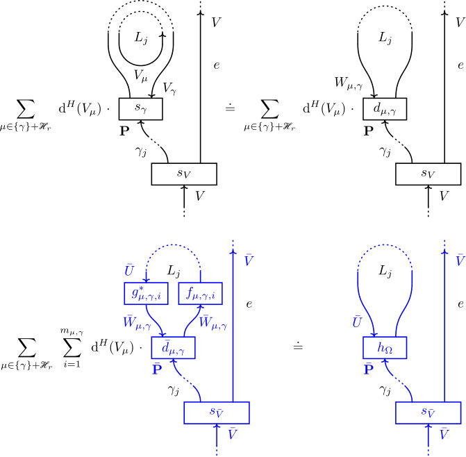 Figure 1
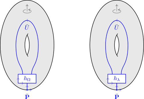 Figure 2
 Figure 3
 Figure 4
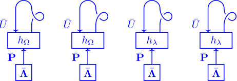 Figure 5
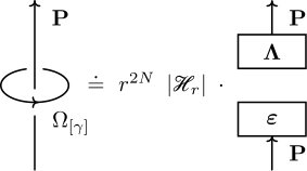 Figure 6
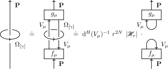 Figure 7
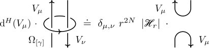 Figure 8
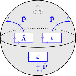 Figure 9
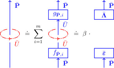 Figure 10
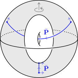 Figure 11
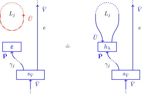 Figure 12
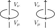 Figure 13
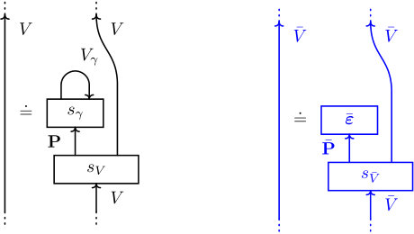 Figure 14
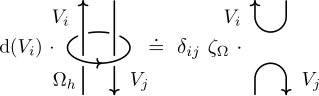 Figure 15
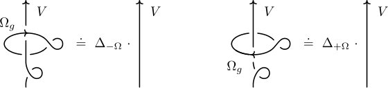 Figure 16
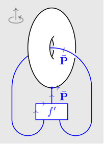 Figure 17
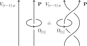 Figure 18
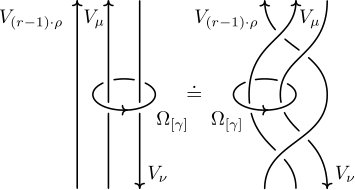 Figure 19
Peer Reviews
No public reviews on file for this paper yet. If you reviewed it on a platform where reviews are public (OpenReview, ICLR, NeurIPS, ICML), you can paste yours below so the community can read it here.
Videos
No videos yet. Explain this paper in a talk, walkthrough, or lecture? Add one.
Taxonomy
TopicsAlgebraic structures and combinatorial models · Advanced Operator Algebra Research · Homotopy and Cohomology in Algebraic Topology
Non-Semisimple Quantum Invariants and TQFTs from Small and Unrolled Quantum Groups
Marco De Renzi
Department of Mathematics, Faculty of Science and Engineering, Waseda University, 3-4-1 Ōkubo, Shinjuku-ku, Tokyo, 169-8555, Japan
,
Nathan Geer
Mathematics & Statistics
Utah State University
Logan, Utah 84322, USA
and
Bertrand Patureau-Mirand
Univ. Bretagne - Sud, UMR 6205, LMBA, F-56000 Vannes, France
Abstract.
We show that unrolled quantum groups at odd roots of unity give rise to relative modular categories. These are the main building blocks for the construction of 1+1+1-TQFTs extending CGP invariants, which are non-semisimple quantum invariants of closed 3-manifolds decorated with ribbon graphs and cohomology classes. When we consider the zero cohomology class, these quantum invariants are shown to coincide with the renormalized Hennings invariants coming from the corresponding small quantum groups.
March 16, 2024
The goal of this paper is two-fold: first of all, we provide a new family of concrete examples of relative modular categories. These are ribbon categories which can be used as fundamental bricks for the construction of non-semisimple quantum invariants of closed manifolds in dimension 3 [5] and Extended Topological Quantum Field Theories (ETQFTs) in dimension 1+1+1 [8]. They are modeled on categories of finite-dimensional weight representations of the unrolled quantum group at even roots of unity , which were used in [2] to build TQFTs in dimension 2+1. They should be thought of as a non-semisimple analogue to standard modular categories, although differences with respect to their semisimple counterparts are many: first of all, a relative modular category comes equipped with a structure group that provides a grading on its objects; secondly, it enjoys finiteness properties only up to the action of a periodicity group of transparent objects; more importantly, it is only generically semisimple, with non-semisimple part confined to a critical set whose complement is dense in . When and the definition reduces to the standard one of [32], see Section 1.7 of [8]. In Theorem 1.3 we prove that categories of finite-dimensional weight representations of unrolled quantum groups associated with arbitrary simple complex Lie algebras at odd roots of unity are relative modular. These categories were already known to induce topological invariants of certain decorated closed 3-manifolds , where is a -colored ribbon graph, where is a cohomology class, and where the triple is subject to a crucial admissibility condition. These so-called Costantino-Geer-Patureau (CGP) quantum invariants are quite rich, but their definition involves certain technical aspects, such as the notion of computable surgery presentation introduced in [5]. The results of this paper imply these invariants can be extended to graded 1+1+1-TQFTs for all simple complex Lie algebras . In the case of , these invariants contain the Akutsu-Deguchi-Ohtsuki invariants of colored links and the abelian Reidemeister torsion of closed 3-manifolds, and they were already known to extend to graded 1+1+1-TQFTs.
The second main result of this paper is a Hennings-type formula for these CGP quantum invariants. More precisely, every simple complex Lie algebra also determines a corresponding small quantum group for every odd root of unity [26, 27]. These finite-dimensional factorizable quotients have been studied a lot in literature [28, 24, 25], and they induce renormalized Hennings TQFTs in dimension 2+1, see [9]. In particular, their categories of finite-dimensional representations yield quantum invariants of certain admissible closed 3-manifolds , where is a -colored bichrome graph, which is a very mild generalization of standard ribbon graphs obtained by specifying special components which correspond to surgery presentations. Then, we prove in Theorem 1.4 that, for a fixed simple complex Lie algebra at an odd root of unity , the CGP invariant of decorated closed 3-manifolds with zero cohomology classes coincides with the corresponding renormalized Hennings invariant . This result builds a bridge between the two theories, and, in this setting, it gives us a way of computing CGP quantum invariants which bypasses computable surgery presentations.
Acknowledgments
We would like to thank the referee for their extremely careful review of our paper. Their deep understanding of our results and their detailed comments helped us improve the paper. NG was partially supported by NSF grants DMS-1308196 and DMS-1452093.
1. Overview of non-semisimple constructions
In this section, we quickly review the two main constructions this paper deals with. References are provided by [5, 2, 8] for the CGP theory, and by [9] for the renormalized Hennings one. All the manifolds we consider are always assumed to be oriented.
1.1. Ribbon categories and m-traces
First, let us fix our notation and conventions for categorical structures. Following [11], a ribbon category is a braided rigid monoidal category equipped with a natural transformation , called the twist, satisfying
[TABLE]
for all , where denotes the braiding of . For every we denote with
[TABLE]
its left and right duality morphisms, and for every we denote with its categorical trace. As shown in [32], every ribbon category induces a ribbon functor called the Reshetikhin-Turaev functor, where denotes the category of -colored ribbon graphs.
An ideal of is a full subcategory of whose class of objects is closed under retracts and absorbent under tensor products with arbitrary objects of . We denote with the ideal of projective objects of . We define the partial trace of an endomorphism to be the endomorphism given by
[TABLE]
Then, following [14, 16], if is a ribbon linear category over a field , an m-trace on is a family of linear maps satisfying:
- (1)
Cyclicity: for all objects and for all morphisms and ; 2. (2)
Partial trace: for all objects and and for every morphism .
For every we denote with its modified dimension. We say an m-trace on is non-degenerate if, for every and , the bilinear pairing is non-degenerate.
Finally, let us fix some terminology which will be extensively used throughout the paper: every time we have a ribbon linear category over a field , we have an associated notion of skein equivalence between formal linear combinations of -colored ribbon graphs. Indeed, if and are objects of , if are scalar coefficients in , and if are morphisms of from and , then we say two formal linear combinations and are skein equivalent, and we write
[TABLE]
if we have the equality under the Reshetikhin-Turaev functor .
1.2. 3-Manifold invariants from non-degenerate relative pre-modular categories
Let us start by recalling the definition of relative pre-modular categories, which, as we mentioned earlier, are ribbon linear categories carrying additional structures. First of all, if is an abelian group, a compatible -structure on a rigid monoidal category is an equivalence of linear categories for a family of full subcategories of satisfying the following conditions: If , then ; If and , then ; If and with , then . Remark that, if is ribbon, then is also ribbon. Next, if is an abelian group, a free realization of in a ribbon category is a monoidal functor , where also denotes the discrete category over with tensor product given by the group operation , satisfying for every , and inducing a free action on isomorphism classes of simple objects of by tensor product with . Next, we say a subset of is symmetric if , and we say it is *small * if for all and all .
Definition 1.1** ([8]).**
If and are abelian groups, and if is a small symmetric subset, then a pre-modular -category relative to is a ribbon linear category over a field together with a compatible -structure on , a free realization , and a non-zero m-trace on . These data are subject to the following conditions:
- (1)
Generic semisimplicity. For every the homogeneous subcategory is semisimple and dominated by for some finite set of simple projective objects with epic evaluation; 2. (2)
Compatibility. There exists a bilinear map such that for every , for every , and for every .
The group is called the structure group, the group is called the periodicity group, and the set is called the critical set of . Condition (1) implies that, for any , every object of is a direct sum of simple objects in the set . We point out that the bilinear map is uniquely determined by the braiding and by the free realization , and that, although the set of representatives is not unique in general, its choice does not affect the following construction. In particular, both and should not be considered relevant parts of the structure of . Relative pre-modular -categories are a slight generalization of the notion of relative -modular category introduced for the first time in [5], see Section 1.5 of [8] for a full discussion of the relation between the two definitions. The change in terminology is motivated by the semisimple theory, where quantum invariants are defined for any non-degenerate pre-modular category, and modularity is an additional condition ensuring the invariant extends to a TQFT. If is a pre-modular -category relative to then the associated Kirby color of index is the formal linear combination of objects
[TABLE]
The name comes from Lemmas 5.9 and 5.10 of [5]. In particular, there exist constants , called stabilization coefficients, which realize the skein equivalences of Figure 1, and which are independent of both and . We say the relative pre-modular category is non-degenerate if .
In [5, 8] it is shown that every non-degenerate relative pre-modular category gives rise to a topological invariant of admissible triples , where is a closed 3-manifold, is a -colored ribbon graph, and is a compatible cohomology class, meaning that every edge is colored with an object of for the homology class of a positive meridian of . The CGP invariant is defined only for admissible triples , which are triples such that every component of contains either a projective edge of , that is an edge of whose color is a projective object of , or a generic curve for , that is an embedded closed oriented curve whose homology class is sent to by . Its definition uses computable surgery presentations in , which are surgery presentations of satisfying for all integers , where denotes the homology class of a meridian of the component . We interpret a surgery presentation of which is computable with respect to some decoration as a -colored ribbon graph by arbitrarily choosing orientations, and by labeling every component with the corresponding Kirby color, with index prescribed by the evaluation of against the homology class of a positive meridian. This is a technical complication, because arbitrary surgery presentations are not computable in general. Computable surgery presentations do exist for admissible decorated closed 3-manifolds, but only up to replacing admissible decorations via certain operations called projective and generic stabilizations, see Section 3.1 of [8]. The idea is to build out of a renormalized invariant of admissible closed -colored ribbon graphs which combines the Reshetikhin-Turaev functor on with the m-trace on . We say a closed -colored ribbon graph is admissible if one of his edges is projective. Example 3 of Section 1.5 in [18] (see also [19, 14, 20]) implies the formula
[TABLE]
defines a topological invariant of the admissible closed -colored ribbon graph , where is projective, and where is a cutting presentation of , i.e. an endomorphism of in whose trace is . Then, for a fixed choice of a square root of , the formula
[TABLE]
defines a topological invariant of the admissible triple thanks to Proposition 3.1 of [8], where is an -component surgery presentation of of signature which is computable with respect to an admissible decoration obtained from by performing projective or generic stabilization, and where .
1.3. 2+1-TQFTs from relative modular categories
A stronger non-degeneracy condition is required in order to extend CGP invariants to graded TQFTs.
Definition 1.2** ([8]).**
A pre-modular -category relative to is relative modular if there exists a relative modularity parameter realizing the skein equivalence of Figure 2 for all and for all .
This condition automatically implies non-degeneracy, because the relative modularity parameter satisfies , see [8]. When is relative modular then, as explained in Section 6.2 of [8], extends to a -graded 2+1-TQFT via a -graded refinement of the universal construction of [3], where is the category of admissible cobordisms of dimension 2+1, and where is the category of -graded vector spaces. More precisely, an object of is a 5-tuple \mathbin{\text{\includegraphics[height=0.0pt]{bbSigma.pdf}}}=(\varSigma,P,\vartheta,B,\mathcal{L}), where is a closed surface, where is a -colored ribbon set, where is a compatible cohomology class, where is a finite set composed of exactly one base point in every connected component of , and where is a Lagrangian subspace. A morphism of from to is an equivalence class of admissible 4-tuples , where is a 3-dimensional cobordism from to , where is a -colored ribbon graph from to , where is a compatible relative cohomology class restricting to and on the incoming and outgoing boundary of respectively, and where is a signature defect. A 4-tuple is admissible if every component of which is disjoint from the incoming boundary contains either a projective edge of , or a generic curve for , and two 4-tuples and are equivalent if , and if there exists a positive diffeomorphism which preserves boundary identifications and satisfies and . Then, can be extended to an invariant of closed morphisms of by setting
[TABLE]
Remark that the category thus obtained is not rigid, as objects such that does not contain any projective point and such that does not admit any generic curve are not dualizable.
State spaces associated with objects of by the -graded TQFT can be described in skein theoretical terms in all degrees. We have two relevant notions of skein equivalence between morphisms of from \mathbin{\text{\includegraphics[height=0.0pt]{bbSigma.pdf}}} to \mathbin{\text{\includegraphics[height=0.0pt]{bbSigma.pdf}}}^{\prime}, one which is local, the other which is not. Indeed, we say a formal linear combination of morphisms of from \mathbin{\text{\includegraphics[height=0.0pt]{bbSigma.pdf}}} to \mathbin{\text{\includegraphics[height=0.0pt]{bbSigma.pdf}}}^{\prime} is a local skein relation if it can be written in the form
[TABLE]
for some coefficients , for some -colored ribbon set with at least one point labeled by a projective object, for some morphism of from (S^{2},P,\vartheta,\{0\})\operatorname{\sqcup}\mathbin{\text{\includegraphics[height=0.0pt]{bbSigma.pdf}}} to \mathbin{\text{\includegraphics[height=0.0pt]{bbSigma.pdf}}}^{\prime}, and for some -colored ribbon graphs from to satisfying
[TABLE]
with respect to some embedding mapping into . Here the cohomology classes and are uniquely determined by and by respectively. On the other hand, we say a formal linear combination of morphisms of from \mathbin{\text{\includegraphics[height=0.0pt]{bbSigma.pdf}}} to \mathbin{\text{\includegraphics[height=0.0pt]{bbSigma.pdf}}}^{\prime} is a non-local skein relation if it can be written in the form
[TABLE]
for some and for some framed knot of color , where is induced by the inclusion of into , and where denotes the homology class of in . Then, if \mathbin{\text{\includegraphics[height=0.0pt]{bbSigma.pdf}}}=(\varSigma,P,\vartheta,B,\mathcal{L}) is an object of , and if is a 3-dimensional cobordism from to , the admissible skein module \check{\mathrm{S}}(M;\mathbin{\text{\includegraphics[height=0.0pt]{bbSigma.pdf}}}) is the quotient, induced by both local and non-local skein relations, of the free vector space \mathcal{V}(M;\mathbin{\text{\includegraphics[height=0.0pt]{bbSigma.pdf}}}) generated by all pairs such that is a morphism of from to \mathbin{\text{\includegraphics[height=0.0pt]{bbSigma.pdf}}}. The class of a generator of \mathcal{V}(M;\mathbin{\text{\includegraphics[height=0.0pt]{bbSigma.pdf}}}) in \check{\mathrm{S}}(M;\mathbin{\text{\includegraphics[height=0.0pt]{bbSigma.pdf}}}) is denoted . The proof of Proposition 4.5 in [2] can be adapted to show that if and are both connected, then \check{\mathrm{S}}(M;\mathbin{\text{\includegraphics[height=0.0pt]{bbSigma.pdf}}}) is a finite-dimensional vector space. On the other hand, if is a 3-dimensional cobordism from to , we denote with \mathcal{V}^{\prime}(M^{\prime};\mathbin{\text{\includegraphics[height=0.0pt]{bbSigma.pdf}}}) the free vector space generated by all pairs such that is a morphism of from \mathbin{\text{\includegraphics[height=0.0pt]{bbSigma.pdf}}} to . Then, for every , the degree state space \mathbb{V}_{\mathcal{C}}^{k}(\mathbin{\text{\includegraphics[height=0.0pt]{bbSigma.pdf}}}) of a connected object \mathbin{\text{\includegraphics[height=0.0pt]{bbSigma.pdf}}} of satisfies
[TABLE]
with respect to the pairing \langle\cdot,\cdot\rangle_{\mathbin{\text{\includegraphics[height=0.0pt]{bbSigma.pdf}}}\operatorname{\sqcup}\mathbb{S}^{2}_{-k}}:\mathcal{V}^{\prime}(M^{\prime};\mathbin{\text{\includegraphics[height=0.0pt]{bbSigma.pdf}}}\operatorname{\sqcup}\mathbb{S}^{2}_{-k})\otimes\check{\mathrm{S}}(M;\mathbin{\text{\includegraphics[height=0.0pt]{bbSigma.pdf}}}\operatorname{\sqcup}\mathbb{S}^{2}_{-k})\rightarrow\Bbbk defined by
[TABLE]
where is a connected 3-dimensional cobordism from to , where is a connected 3-dimensional cobordism from to , and where the object
[TABLE]
of is determined by the -colored ribbon set composed of three points in standard positions with orientations and colors specified by their subscript for some and for some . Remark that an explicit characterization of these quotients can sometimes be achieved. For instance, if is a -colored ribbon set composed of a single positive point of color , then, thanks to Remark 7.2 of [8], the -graded state space of the object of satisfies
[TABLE]
where for all we denote with the -graded vector space whose space of degree vectors is given by for every . See also Proposition 7.16 of [8] for a description, in terms of homogeneous colorings of trivalent graphs, of the -graded state space of generic surfaces in .
1.4. 3-Manifold invariants from finite-dimensional non-degenerate unimodular ribbon Hopf algebras
Next, let us move on to the renormalized Hennings theory. We start by fixing our notation for Hopf algebras, and by recalling some crucial definitions and results. If is a field, a finite-dimensional ribbon Hopf algebra is a finite-dimensional vector space over endowed with a multiplication , a unit , a coproduct , a counit , an antipode , an R-matrix , and a ribbon element in the center of , see [31] for a list of the axioms these structure maps and elements are subject to. We use the notation for every and , and we denote with the Drinfeld element, and with the pivotal element associated with the ribbon structure of . As a consequence of finite-dimensionality, admits a right integral and a left cointegral which are unique up to scalar, and we can fix a pair satisfying . The Hopf algebra is non-degenerate if the stabilization coefficients and satisfy , and it is unimodular if the left cointegral is two-sided, meaning that it is also a right cointegral. The category -mod of finite-dimensional left -modules is a ribbon linear category, with evaluation and coevaluation morphisms given by
[TABLE]
for every left -module with basis and dual basis , and with braiding morphisms given by
[TABLE]
for all left -modules and . Thanks to Theorem 1 of [1], admits an m-trace on the ideal of projective -modules , which is unique up to scalar and uniquely determined by the condition for all , where denotes the regular representation of . Furthermore, is non-degenerate.
In [9] it is shown that every finite-dimensional non-degenerate ribbon Hopf algebra gives rise to a topological invariant of admissible pairs , where is a closed 3-manifold, and is a -colored bichrome graph. The latter are -colored ribbon graphs carrying a set of specified edges, and their name comes from the fact that we think about special edges as being red, while the rest of the graph is blue. Red edges can only be colored with the regular representation , and they can only intersect coupons in a prescribed way: for every coupon of a bichrome graph there exists an integer such that the first input edges are incoming and red, the first output edges are outgoing and red, while all the other ones are blue. Such a coupon is colored with a morphism in the -th stabilized subcategory of , which is the category whose objects have the form for some , and whose morphisms have the form for some left translation by and for some linear map . The ribbon category of -colored bichrome graphs provides a graphical calculus which is formalized by the Hennings-Reshetikhin-Turaev functor introduced in Proposition 2.5 of [9]. By definition, coincides with the Reshetikhin-Turaev functor in the absence of red edges, it coincides with the Hennings invariant in the absence of blue edges, and it coherently combines the two behaviors for general -colored bichrome graphs. Remark that yields a notion of skein equivalence between formal linear combinations of -colored bichrome graphs in the same way does for -colored ribbon graphs. This way, is naturally identified with the subcategory of whose morphisms are entirely blue. The renormalized Hennings invariant is then defined only for admissible pairs , which are pairs such that every component of contains a projective blue edge of . Its definition uses surgery presentations in , which we interpret as -colored bichrome graphs by arbitrarily choosing orientations, by labeling every component with the regular representation , and by taking them to be red. The idea is to build out of a renormalized invariant of admissible closed -colored bichrome graphs which combines the Hennings-Reshetikhin-Turaev functor on with the m-trace on . We say a closed -colored bichrome graph is admissible if one of his blue edges is projective. The formula
[TABLE]
defines a topological invariant of the admissible closed -colored bichrome graph thanks to Theorem 2.7 of [9], where is a projective object of , and where is a cutting presentation of , meaning an endomorphism of in whose trace is . Then, for a fixed choice of a square root of , the formula
[TABLE]
defines a topological invariant of the admissible pair thanks to Theorem 2.9 of [9], where is an -component surgery presentation of of signature , and where .
1.5. 2+1-TQFTs from finite-dimensional factorizable ribbon Hopf algebras
A finite-dimensional ribbon Hopf algebra with R-matrix is factorizable if the Drinfeld map , which is defined by
[TABLE]
for every , is an isomorphism. This condition implies both non-degeneracy and unimodularity, see [21] and [31]. When is factorizable then, as explained in Section 3 of [9], extends to a 2+1-TQFT via the universal construction of [3], where is the category of admissible cobordisms of dimension 2+1. More precisely, an object of is a triple \mathbin{\text{\includegraphics[height=0.0pt]{bbSigma.pdf}}}=(\varSigma,P,\mathcal{L}), where is a closed surface, where is a blue -colored ribbon set, and where is a Lagrangian subspace. A morphism of from to is an equivalence class of admissible triples , where is a 3-dimensional cobordism from to , where is a -colored bichrome graph from to , and where is a signature defect. A triple is admissible if every component of which is disjoint from the incoming boundary contains a projective blue edge of , and two triples and are equivalent if , and if there exists a positive diffeomorphism which preserves boundary identifications and satisfies . Then, can be extended to an invariant of closed morphisms of by setting
[TABLE]
Remark that the category thus obtained is not rigid, as objects such that does not contain any projective blue point are not dualizable.
State spaces associated with objects of by the TQFT can be presented as quotients of admissible skein modules, just like we did in the CGP case, and of course this time only local skein relations are needed. However, they can also be efficiently described in terms of the dual coadjoint -module , which is the vector space equipped with the action for all and . Indeed, if is a left -module with action , we can consider its subspace of -invariant vectors, which is defined as
[TABLE]
Remark that we have an obvious isomorphism between \mathrm{Hom}_{\mathcal{C}}(\mathbin{\text{\includegraphics[height=0.0pt]{bb1.pdf}}},V) and sending to . Then, if is a closed surface of genus , and if is a single positive framed blue point of color , it follows directly from Corollary 3.21 of [9] that the state space of the object \mathbin{\text{\includegraphics[height=0.0pt]{bbSigma.pdf}}}_{g,V}=(\varSigma_{g},P_{V},\mathcal{L}) of determined by any arbitrary Lagrangian satisfies
[TABLE]
1.6. Main results
As we mentioned earlier, this paper contains two main results related to the non-semisimple constructions we just recalled. The first one concerns the existence of a family of graded TQFTs, as well as graded ETQFTs, for the CGP theory. The setting is provided by unrolled quantum groups at odd roots of unity. More precisely, in Subsection 2.2 we recall the definition, for every simple complex Lie algebra of rank and dimension , of a particular quantum deformation, denoted , of the enveloping algebra for , where is an odd integer which is required not to be a multiple of 3 when . These unrolled quantum groups are quite different from the ones which usually underlie quantum constructions in low dimensional topology. For instance, they are infinite dimensional: indeed, they are generated by , but while generators and , as well as their induced root vectors, are set to be nilpotent, generators and are not required to be quasi-unipotent. This produces a representation theory in which weights are allowed to take arbitrary complex values, instead of integral ones. As a consequence, we need to be careful when it comes to defining braidings of representations. Indeed, we need the presence of generators , which should be thought of a logarithms of generators . This exponential relation is not set at the level of the quantum group, but we restrict to representations where it is satisfied. More precisely, we focus on the full subcategory of finite-dimensional representations of where the action of generators is diagonalizable, and where the action of generators is obtained by exponentiating. This category is non-semisimple, and it was studied in detail in [17]: a full subcategory of was proven to be ribbon, and the equality was conjectured. In [5], it was shown that is non-degenerate relative pre-modular, and thus yields a quantum invariant of admissible decorated 3-manifolds. In [18], the conjecture was proven: is a relative pre-modular category. Its structure group is given by , where is a Cartan subalgebra of with root lattice . Its periodicity group is given by , where denotes the weight lattice. Its critical set is given by , where is a set of positive roots of . The following is our first main result, which implies, as an immediate consequence, the existence of a -graded ETQFT in dimension 1+1+1 extending the quantum invariant .
Theorem 1.3**.**
The category is relative modular.
The second main result of this paper builds a bridge between this family of quantum invariants and the renormalized Hennings ones coming from the corresponding small quantum groups, under the additional assumption that , where denotes the Cartan matrix of . Indeed, in Subsection 2.1 we recall the definition of a more classical quantum version of , denoted , again for . These small quantum groups are far better known: they are finite-dimensional, as generators and are set to be quasi-unipotent, they are ribbon and factorizable, and thus they yield TQFTs in dimension 2+1. The category of finite-dimensional representations of is still non-semisimple, but all weights take integral values. Indeed, we have a very natural forgetful functor from the full subcategory of whose objects have all weights in to : the image of an object of is simply defined by forgetting the action of generators . The technical condition ensures is essentially surjective. Furthermore, immediately induces a functor from to : the image of a morphism of is simply defined by applying the forgetful functor to all its colors.
Theorem 1.4**.**
If is a closed 3-manifold and is an admissible -colored ribbon graph, then
[TABLE]
We point out that each invariant depends on the choice of a square root of the product of the stabilization coefficients for the corresponding version of the quantum group. Theorem 1.4 requires a coherent choice of these square roots in the two theories, otherwise a sign will appear in the relation. Remark also that a great advantage of the renormalized Hennings theory is the absence of many technical complications which characterize the CGP one. For instance, arbitrary surgery presentations can be used to define and compute quantum invariants associated with small quantum groups, as we have no computability condition. Therefore, Theorem 1.4 gives a convenient alternative formulation for the CGP invariants associated with unrolled quantum groups, at least in the case of 3-manifolds decorated with the trivial cohomology class.
Let us end this introduction with a final comment about our choice for the setting of Theorem 1.4. When we started writing these results, the renormalized Hennings construction had only been developed in the case of finite-dimensional factorizable ribbon Hopf algebras. As a consequence, a comparison with the CGP construction had to take place in this context. The classification of finite-dimensional factorizable quantum groups is not so easy, see [25], and we choose for simplicity to limit ourselves to the smallest set of Cartan generators at odd roots of unity. However, a recent generalization of the renormalized Hennings construction allows us to consider arbitrary modular categories, in the non-semisimple sense, as building blocks for non-semisimple 2+1-TQFTs [10]. This larger setting encompasses examples of ribbon categories coming from the representation theory of restricted quantum groups at even roots of unity. Indeed, while some of these Hopf algebras might not be braided [24, 25], a suitable modification of their coalgebra structure produces quasi-Hopf deformations which admit a ribbon structure [6, 13, 30]. For what concerns unrolled quantum groups, even roots of unity have been less studied due to several technical difficulties which produce fascinating but complicated phenomena in the theory. It would be very interesting to generalize Theorem 1.4 to this setting, and possibly to even larger ones.
2. Quantum groups at odd roots of unity
In this section we recall definitions of small and unrolled quantum groups associated with arbitrary simple complex Lie algebras , and we prove our first result: categories of finite-dimensional weight representations of unrolled quantum groups at odd roots of unity are relative modular, and can therefore be used to construct ETQFTs in dimension 1+1+1.
2.1. Small quantum groups
Let be a simple complex Lie algebra of rank and dimension , let be a Cartan subalgebra of , let be a set of positive roots of , and let be the associated quantum group, over a formal parameter , introduced in Appendix A. Let us fix an odd integer with the further condition that modulo if , and let us specialize to in the De Concini-Kac sense [7]. Let denote the small quantum group of , which is the -algebra obtained from by adding relations
[TABLE]
for every and every . Then inherits from the structure of a Hopf algebra, and we denote with , with , and with the subalgebras of generated by , by , and by , respectively. As proved in [26], see also Theorem 30 of [17], a Poincaré-Birkhoff-Witt basis is given by
[TABLE]
so is finite-dimensional. A pivotal element is given by where
[TABLE]
Furthermore, if we consider given by
[TABLE]
and given by
[TABLE]
then is an R-matrix for , as proved in [26], see also [25]. Next, thanks to Proposition A.5.1 of [28], a right integral of is given by
[TABLE]
This formula can be deduced from the one in [28] by remarking that Lyubashenko uses Luszitg’s coproduct , where denotes the involutive algebra automorphism of defined by and by for all integers , and by remarking that is a right integral for if and only if is a left integral for . Finally, thanks to Proposition A.5.2 of [28], a two-sided cointegral of satisfying is given by
[TABLE]
Proposition 2.1**.**
The Hopf algebra is factorizable and ribbon.
This result is proved in [28], see also [25]. We denote with the ribbon category of finite-dimensional -modules, and with the m-trace on given by Theorem 1 of [1], which satisfies for the regular representation of .
Corollary 2.2**.**
The renormalized Hennings invariant extends to a TQFT
[TABLE]
2.2. Unrolled quantum groups
Let denote the unrolled quantum group of , which is the -algebra obtained from by adding generators
[TABLE]
and relations
[TABLE]
for every integer and every positive root . Then can be made into a pivotal Hopf algebra by setting
[TABLE]
for every integer , and we denote with , with , and with the subalgebras of generated by , by , and by respectively. For every let us introduce the notation
[TABLE]
A -module with action is a weight module if it is a semisimple -module and if for every and every we have
[TABLE]
where we are identifying with the corresponding linear subspace of in the obvious way. We denote with the full subcategory of the category of finite-dimensional -modules whose objects are weight modules. Then can be made into a ribbon category as follows: first of all, a pivotal element is given by , where the choice of the exponent is explained in Remark 4 of [18]. Furthermore, if and are objects of , their braiding morphism is given by
[TABLE]
for the linear maps and determined by
[TABLE]
for all , satisfying
[TABLE]
for every integer , and for . Thanks to Theorem 4 of [18], is a ribbon category.
If we set , then supports the structure of a -category: indeed, for every we can define the homogeneous subcategory to be the full subcategory of with objects given by modules whose weights are all of the form for some . Furthermore, if we set , then we have a free realization mapping every to the object given by the vector space with -action specified by
[TABLE]
for every integer . Now the bilinear map
[TABLE]
satisfies for every , every , and every . If we consider the critical set
[TABLE]
then, as explained in Section 7 of [5], the category is semisimple for every . Therefore, the last relevant piece of structure we are missing is an m-trace. In order to define it, let us introduce typical -modules. First of all, we say a vector of a -module is a highest weight vector if for every integer . Analogously, we say a vector of is a lowest weight vector if for every integer . Then for every weight there exists a simple finite-dimensional weight -module featuring a highest weight vector of weight . This module is unique up to isomorphism, and every simple weight -module is of this form, see Proposition 33 of [17]. Every such module also has a lowest weight vector, and it is called typical if its lowest weight is given by . If we consider the set
[TABLE]
then, thanks to Proposition 34 of [17], is typical if and only if . Remark that if satisfies for every , then . This means that if satisfies , then is typical. We also point out that, although , the module is always typical, because
[TABLE]
is not in for any integer . Now, thanks to Lemma 7.1 of [5] and Theorem 38 of [17], every typical -module is projective and ambidextrous. Then, by combining Theorem 3.3.2 of [14] with Lemma 17 of [20], there exists a non-zero m-trace on the ideal of projective objects of which is unique up to scalar. Therefore, we can fix the normalization . Thanks to Equation (51) and Lemma 47 of [17], for every we have
[TABLE]
For all , if and for the -colored ribbon graphs and represented in Figure 3, Proposition 45 of [17] gives
[TABLE]
and, since , it also gives
[TABLE]
2.3. Relative modularity
In this subsection we will prove the category is relative modular, and thus yields a -graded TQFT. In order to do this, we will first need a preliminary definition. We say an endomorphism of an object of is transparent in if for all objects we have
[TABLE]
Lemma 2.3**.**
If is transparent in , then there exist some integer and some morphisms and for every integer such that
[TABLE]
Proof.
If is a highest weight vector of and is a weight vector of then is proportional to because
[TABLE]
for all integers whose sum is strictly positive. Furthermore, is proportional to because is transparent in . But now
[TABLE]
is a basis of thanks to Proposition 34 of [17]. This means that
[TABLE]
for every weight vector and for all integers whose sum is strictly positive.
Analogously, if is a lowest weight vector of and is a weight vector of then is proportional to because
[TABLE]
for all integers whose sum is strictly positive. Furthermore, is proportional to because is transparent in . But now
[TABLE]
is a basis of thanks to Proposition 34 of [17]. This means that
[TABLE]
for every weight vector and for all integers whose sum is strictly positive.
Now, since for every integer , we get the equality for every , which implies
[TABLE]
Then, if is a weight vector of weight , this tells us that for every integer . Since is odd and coprime with for every integer , this means precisely that . Therefore, each weight vector of determines a 1-dimensional submodule which is isomorphic to for some . Since is a direct sum of its weight spaces, this means that
[TABLE]
for some integer and some . Let and denote the corresponding projection and injection morphisms for every integer . We can factorize where is naturally induced by and denotes inclusion. Then the result follows by setting and for every integer . ∎
Let us complete to a set of representatives of equivalence classes in . Similarly, let us choose a set of representatives of equivalence classes in . If for every we define , then
[TABLE]
is a set of representatives of -orbits of isomorphism classes of simple objects of . We have now everything in place to prove Theorem 1.3.
Proof of Theorem 1.3.
We know is a non-degenerate relative pre-modular category thanks to Theorem 7.2 of [5] and to Theorem 4 of [18]. Therefore, we only need to prove that satisfies the relative modularity condition of Definition 1.2. We will do this by showing the skein equivalence of Figure 4 for every , for every , and for every , so let denote the morphism of obtained by applying the Reshetikhin-Turaev functor to the -colored ribbon graph represented in the left hand part of Figure 4, ignoring the coefficient. Thanks to the handle slide property, we have the skein equivalence of Figure 5,
which means is transparent in . Now, thanks to Lemma 2.3, we have
[TABLE]
with , with , and with for every integer . But now unless and , because
[TABLE]
and because is a set of representatives of equivalence classes in . This means that factors through the tensor unit \mathbin{\text{\includegraphics[height=0.0pt]{bb1.pdf}}}. But now, since is simple, both \mathrm{Hom}_{\mathcal{C}^{H}}(V_{\mu}\otimes V_{\mu}^{*},\mathbin{\text{\includegraphics[height=0.0pt]{bb1.pdf}}}) and \mathrm{Hom}_{\mathcal{C}^{H}}(\mathbin{\text{\includegraphics[height=0.0pt]{bb1.pdf}}},V_{\mu}\otimes V_{\mu}^{*}) are 1-dimensional. This means is a scalar multiple of . In order to compute the proportionality coefficient let us compare the m-traces of and of . The first m-trace is easily seen to be
[TABLE]
Indeed, this follows immediately from the partial trace property of . On the other hand, if
[TABLE]
where is obtained from by replacing the label of the meridian with , then, the second m-trace is given by
[TABLE]
where the morphisms and are represented in Figure 3. Indeed, the second equality follows from both the cyclicity and the partial trace properties of , using isotopy, the third equality follows from the fact that is simple, and the fourth equality follows from the very last equation of Subsection 2.2. ∎
Corollary 2.4**.**
The CGP invariant extends to a -graded TQFT
[TABLE]
2.4. Projective generators and forgetful functor
In this subsection we prove some key technical results which will be later used for the proof Theorem 1.4. We say an object of is a projective generator of if for every object of there exist some integer and some morphisms and for every integer such that
[TABLE]
Remark that a natural choice for a projective generator of is the regular representation of . Analogously, we say an object of is a relative projective generator of if for every object of there exist some integer , some , and some morphisms and for every integer such that
[TABLE]
Next, we apply the following result to .
Proposition 2.5**.**
Let be an abelian relative pre-modular -category over an algebraically closed field . Then has enough projectives, and every indecomposable projective object is a projective cover of a simple object.
Proof.
Choose some and some simple object . By definition is semisimple, and so is projective and has epic evaluation. Then for every the morphism
[TABLE]
is an epimorphism from a projective object to . Thus has enough projectives. Next, for the second statement, let be an indecomposable projective object of for some . Since is small in , there exists some satisfying . Then, let be a simple object of . The algebra embeds into with bounded by the number of simple summands of . Then Fitting’s Lemma applies to , i.e. its elements are either nilpotent or isomorphisms. We can now prove that has a unique maximal proper subobject. To see this, let us suppose by contradiction and are distinct maximal proper subobjects. Then we have an epimorphism which admits a section , because is projective. If denotes the inclusion and , then . Since their sum is the identity of , they commute, and and cannot be simultaneously nilpotent. Thanks to Fitting’s Lemma, is an isomorphism for some . This implies that is a retract of , and thus is a proper subobject of . Then is a proper subobject of itself, but is also semisimple, which is a contradiction. ∎
We will denote by a projective cover of for any . Thanks to Proposition 2.5, if denotes the set of representatives of equivalence classes in of Figure 4, then
[TABLE]
is by construction a relative projective generator of .
Lemma 2.6**.**
* for every .*
Proof.
Since the vector space of -module morphisms from a projective indecomposable weight -module to its unique simple quotient is 1-dimensional, and since is the -orbit of the tensor unit \mathbin{\text{\includegraphics[height=0.0pt]{bb1.pdf}}}, we have
[TABLE]
Furthermore, since the dual of an indecomposable projective weight -module is also indecomposable and projective, see for instance Proposition 6.1.3 of [11], Proposition 2.5 implies that each indecomposable projective weight -module has an unique simple submodule which is dual to the simple quotient of . Since is unimodular, see [17] and Theorem 3.1.3 of [15], is the unique indecomposable projective weight -module that constains the tensor unit \mathbin{\text{\includegraphics[height=0.0pt]{bb1.pdf}}}=\sigma(0) as a submodule, and similarly is the unique indecomposable projective weight -module that contains as a submodule. Hence we have
[TABLE]
The following result establishes a cutting property for Kirby meridians which is analogous to Lemma 3.6 of [9].
Lemma 2.7**.**
There exist generators \boldsymbol{\varepsilon}\in\mathrm{Hom}_{\mathcal{C}^{H}}(\mathbf{P},\mathbin{\text{\includegraphics[height=0.0pt]{bb1.pdf}}}) and \mathbf{\Lambda}\in\mathrm{Hom}_{\mathcal{C}^{H}}(\mathbin{\text{\includegraphics[height=0.0pt]{bb1.pdf}}},\mathbf{P}) satisfying which realize the skein equivalence of Figure 6.
Proof.
Thanks to Lemma 2.6, and thanks to the non-degeneracy of , the composition of a non-trivial morphism of \mathrm{Hom}_{\mathcal{C}^{H}}(\mathbf{P},\mathbin{\text{\includegraphics[height=0.0pt]{bb1.pdf}}}) with a non-trivial morphism of \mathrm{Hom}_{\mathcal{C}^{H}}(\mathbin{\text{\includegraphics[height=0.0pt]{bb1.pdf}}},\mathbf{P}) has non-zero m-trace. Therefore, let us fix a pair of generators \boldsymbol{\varepsilon}\in\mathrm{Hom}_{\mathcal{C}^{H}}(\mathbf{P},\mathbin{\text{\includegraphics[height=0.0pt]{bb1.pdf}}}) and \mathbf{\Lambda}\in\mathrm{Hom}_{\mathcal{C}^{H}}(\mathbin{\text{\includegraphics[height=0.0pt]{bb1.pdf}}},\mathbf{P}) satisfying , and let us prove they realize the skein equivalence of Figure 6. If is the morphism of obtained by applying the Reshetikhin-Turaev functor to the -colored ribbon graph represented in the left hand part of Figure 6, the handle slide property yields the skein equivalence represented in Figure 7.
This means that, thanks to Lemmas 2.3 and 2.6, the morphism factors through the tensor unit \mathbin{\text{\includegraphics[height=0.0pt]{bb1.pdf}}}. But then, since \mathrm{Hom}_{\mathcal{C}^{H}}(\mathbf{P},\mathbin{\text{\includegraphics[height=0.0pt]{bb1.pdf}}}) and \mathrm{Hom}_{\mathcal{C}^{H}}(\mathbin{\text{\includegraphics[height=0.0pt]{bb1.pdf}}},\mathbf{P}) are both 1-dimensional, we must have for some . Then, let us show . Proposition 2.5 implies \mathrm{Hom}_{\mathcal{C}^{H}}(P_{\mu},\mathbin{\text{\includegraphics[height=0.0pt]{bb1.pdf}}}) is -dimensional for every . Moreover, for every , the projective cover of V_{0}=\mathbin{\text{\includegraphics[height=0.0pt]{bb1.pdf}}} is a direct summand of of multiplicity 1. In other words, we have
[TABLE]
for some weights satisfying and for all integers , and for some -module morphisms and . Remark that this implies
[TABLE]
Therefore, let us fix some , and let us consider the -module morphisms and determined by the projection and the injection . Thanks to Figure 4, we have the skein equivalence of Figure 8.
Then, let us compute the m-trace of in two different ways. On one hand, we have
[TABLE]
On the other hand, we have
[TABLE]
where the second and fifth equalities follow from the cyclicity and the partial trace properties of respectively. ∎
Let us consider the forgetful functor which forgets the action of for all integers . If is an object of we denote with its image under , and if is a morphism of we denote with its image under . This induces a ribbon functor from the category of -colored ribbon graphs to the category of -colored ribbon graphs. If is a morphism of we denote with its image under .
Lemma 2.8**.**
The forgetful functor is ribbon, and it satisfies
[TABLE]
Proof.
First of all, remark that in . Then the result follows immediately from the equality
[TABLE]
for all , where is defined in Subsection 2.2, and where is defined in Subsection 2.1. To show the claim, remark
[TABLE]
for every . This means that
[TABLE]
for all , satisfying
[TABLE]
for every integer . ∎
The forgetful functor preserves the property of being projective.
Lemma 2.9**.**
If is a projective object of , then is a projective object of .
Proof.
The typical -module introduced in Subsection 2.2 generates thanks to Lemma 17 of [20]. Then must be a direct summand of a tensor product for some . Now the proof of Lemma 7.1 of [5] can be repeated to show the image of under the forgetful functor is projective. This means generates , and thus , which is a direct summand of , is projective. ∎
In particular, the image of the relative projective generator of defined in Subsection 2.4 is projective.
Lemma 2.10**.**
\dim_{\mathbb{C}}\left(\mathrm{Hom}_{\bar{\mathcal{C}}}(\mathbin{\text{\includegraphics[height=0.0pt]{bb1.pdf}}},\bar{\mathbf{P}})\right)=\dim_{\mathbb{C}}\left(\mathrm{Hom}_{\bar{\mathcal{C}}}(\bar{\mathbf{P}},\mathbin{\text{\includegraphics[height=0.0pt]{bb1.pdf}}})\right)=1.
Proof.
Let be a weight -module in , and remark that its image under coincides with as a vector space. Let us consider the space of -invariants vectors of . Remark that \mathrm{Hom}_{\bar{\mathcal{C}}}(\mathbin{\text{\includegraphics[height=0.0pt]{bb1.pdf}}},\bar{V}) is naturally isomorphic to , simply by identifying every morphism f\in\mathrm{Hom}_{\bar{\mathcal{C}}}(\mathbin{\text{\includegraphics[height=0.0pt]{bb1.pdf}}},\bar{V}) with the image . We claim the subspace of formed by vectors of is a -submodule of . Indeed, this follows from the commutation relations satisfied by the additional generators . But now remark that every weight vector of with respect to the action of determines a split 1-dimensional submodule of which is isomorphic to for some , as all 1-dimensional weight -modules in are. This means that
[TABLE]
with for every integer . Thus we get
[TABLE]
and the converse inequality follows from the equality \Phi_{\mathcal{C}}(\sigma(\kappa))=\mathbin{\text{\includegraphics[height=0.0pt]{bb1.pdf}}} for every .
First, let us consider . Thanks to Lemma 2.6, we have
[TABLE]
Thus, the space is 1-dimensional. This means
[TABLE]
Next, let us consider . Thanks to Lemma 2.6, we have
[TABLE]
Thus, the space is 1-dimensional. This means
[TABLE]
The last result we will need requires an additional hypothesis.
Proposition 2.11**.**
If , then is a projective generator of .
Proof.
Let us show that every indecomposable projective -module is isomorphic to a direct summand of . Let be the unique simple quotient of . Its highest weight is a ring homomorphism assigning to each the root of unity by which it acts on the highest weight vector of . Since is coprime with defined in Appendix A, there exists some satisfying for every integer . Furthermore, since is coprime also with , the matrix is invertible modulo . In particular, there exist such that modulo for all integers . Then, if we set
[TABLE]
the simple weight -module satisfies , because and have the same highest weight. Moreover, if is a projective cover of , then is isomorphic to a direct summand of for some . But now, since is projective, it must contain as a direct summand, so this proves our statement. ∎
3. Equality of 3-manifold invariants
The goal for this section is to prove Theorem 1.4. We will use as a key ingredient the fact that meridians labeled with Kirby colors have the cutting property with respect to the relative projective generator of , while red meridians labeled with the regular representation have the cutting property with respect to its image in . The proof will require a comparison of all the ingredients that correspond to each other in the two theories. Since it is part of the hypotheses of Theorem 1.4, we will suppose throughout this section that .
3.1. Stabilized surgery presentations
In this subsection we introduce special surgery presentations of admissible decorated closed 3-manifolds which are tailored for the comparison between the CGP and the renormalized Hennings invariants. We start with a preliminary comment about our notation: we will always denote with the restriction of to -colored blue ribbon graphs, and similarly we will always denote with the restriction of to admissible closed -colored blue ribbon graphs, in order to stress the absence of red edges. Next, we need to compare the m-trace on with the m-trace on .
Remark 3.1*.*
Both and are unique up to scalar, but the chosen normalizations do not agree, as they are determined by the conditions
[TABLE]
respectively, where is the relative projective generator of introduced in Subsection 2.4, where \boldsymbol{\varepsilon}\in\mathrm{Hom}_{\mathcal{C}^{H}}(\mathbf{P},\mathbin{\text{\includegraphics[height=0.0pt]{bb1.pdf}}}) and \mathbf{\Lambda}\in\mathrm{Hom}_{\mathcal{C}^{H}}(\mathbin{\text{\includegraphics[height=0.0pt]{bb1.pdf}}},\mathbf{P}) are the morphisms introduced in Lemma 2.7, where is the regular representation of , and where and are the counit and the cointegral respectively. Nevertheless, clearly defines an m-trace on : indeed, it obviously satisfies the cyclicity property, and the partial trace property is just a consequence of the fact that partial traces commute with the ribbon functor (see also Corollary 2.8 of [12] for a similar statment in the setting of finite dimensional Hopf algebras). Therefore, there exists a non-zero coefficient such that
[TABLE]
meaning that for every and every .
Lemma 3.2**.**
The renormalized invariants and satisfy
[TABLE]
meaning that for every closed admissible -colored ribbon graph , where is the coefficient introduced in Remark 3.1.
Proof.
If a closed admissible -colored ribbon graph admits a projective edge of color , and if is a cutting presentation of , then we have
[TABLE]
where the second equality follows from Lemma 2.8. ∎
Now, let us recall the formulas defining the CGP and the renormalized Hennings invariants in the setting of Theorem 1.4. If is a closed connected morphism of , if is a surgery presentation of , and if we replace with some obtained by projective stabilization of sufficiently generic index ensuring becomes computable, as explained in Subsection 1.2 and, in greater detail, in Section 3.2 of [8], then we have
[TABLE]
On the other hand, if is the closed connected morphism of obtained by applying the functor to , then we have
[TABLE]
The surgery presentation is used in different ways by the two constructions. In the first case, is labeled with Kirby colors as prescribed by , and thus it is not a morphism in the domain of . In the second case, is taken to be red, and thus it is not a morphism in the image of . In order to compare the two formulas, we introduce special morphisms of which encode these two different procedures.
First, for all weights satisfying , the tensor product is an object of . Therefore, since is a projective generator of , we can fix a decomposition
[TABLE]
for some morphisms and . Let us also set
[TABLE]
where is a morphism satisfying , and where is the isomorphism coming from the pivotal structure of . Now, let us fix once and for all a weight satisfying . Then we denote with the morphism
[TABLE]
Next, we denote with the unique morphism which sends the generator to , where is the right integral of , and we consider a morphism satisfying . Then we denote with the morphism
[TABLE]
This allows us to review the recipe for the computation of the two invariants. If is a closed morphism of , if is a projective edge of color , and if is a surgery presentation of , then let us fix disjoint paths connecting to for every integer . Before starting, we perform special projective stabilizations both on and on at the intersection point with for every integer , as shown in Figure 9,
where is a section of , where is its image under , and where is a morphism satisfying . Next, we isotope the -colored and the -colored coupons along the path until the intersection point with . This is our initial configuration.
Let us start from the CGP invariant. First, we need to slide every -colored edge along the corresponding component , so to turn the surgery presentation into a computable one. Proposition 3.1 of [8] implies the choice of the weight satisfying is inconsequential. This produces the -colored ribbon graph represented in the top-left corner of Figure 10.
Up to skein equivalence of -colored ribbon graphs, we can replace a tubular neighborhood of as shown in the top-right corner of Figure 10, thus obtaining a -colored ribbon graph. This means we can apply the functor which, up to skein equivalence of -colored ribbon graphs, produces the -colored ribbon graph represented in the bottom-left corner of Figure 10. Again up to skein equivalence of -colored ribbon graphs, we can replace a tubular neighborhood of as shown in the bottom-right corner of Figure 10. The resulting -colored ribbon graph is denoted , and is said to be obtained from the surgery presentation and from the admissible -colored ribbon graph by -stabilization along the paths . By construction, using Lemma 3.2, we have
[TABLE]
Let us move on to discuss the renormalized Hennings invariant. First, we need to interpret every component as a red edge, and to label it with the regular representation . This produces the -colored bichrome graph represented in the left-hand part of Figure 11.
Up to skein equivalence of -colored bichrome graphs, we can turn every red component blue by replacing a tubular neighborhood of as shown in the right-hand side of Figure 11. The resulting -colored ribbon graph is denoted , and is said to be obtained from the surgery presentation and from the admissible -colored ribbon graph by -stabilization along the paths . By construction, using Lemma 3.8 of [9], we have
[TABLE]
Remark that, since and were obtained starting from surgery presentations computing and through operations which do not alter the values of and of respectively, this means that both and are independent of the choice of the paths .
3.2. Stabilization coefficients
Next, we need to compare with , with , and with . In order to do this, we will prove a key technical result. Let be the object of defined by
[TABLE]
where the blue -colored ribbon set is given by a single framed point with negative orientation and color , and where the Lagrangian subspace is generated by the homology class of the curve . Analogously, let be the object of defined by
[TABLE]
where the blue -colored ribbon set is given by three framed points, two with negative, one with positive orientation, and all with color . Let us also consider the morphism of defined by
[TABLE]
where is an open tubular neighborhood of the curve , and where the -colored framed tangle is represented in Figure 12.
Lemma 3.3**.**
The linear map
[TABLE]
is injective.
Proof.
As we will show, the proof follows rather directly from the surjectivity of
[TABLE]
Indeed, a vector of the form
[TABLE]
for some and some is trivial if and only if
[TABLE]
for every , where for every object \mathbin{\text{\includegraphics[height=0.0pt]{bbSigma.pdf}}} of the linear map
[TABLE]
denotes the non-degenerate pairing induced by the universal construction in Section 3.3 of [9]. Then, since
[TABLE]
for every and every , the injectivity of
[TABLE]
is equivalent to the surjectivity of
[TABLE]
In order to prove that is surjective we remark that, as soon as an object \mathbin{\text{\includegraphics[height=0.0pt]{bbSigma.pdf}}}=(\varSigma,P,\mathcal{L}) of features a projective blue point of in every connected component of , the proof of Proposition 3.13 of [9] can be repeated to show that the linear map
[TABLE]
is surjective for every connected 3-dimensional cobordism from to . This means that every vector in can be described by a linear combination of -colored bichrome graphs inside from to . Let be such a -colored bichrome graph. Up to isotoping its -colored edge intersecting , we can make sure there is a projective edge of piercing the solid torus . But now, thanks to Proposition 2.11, is a projective generator of . This means that, up to skein equivalence, we can insert a pair of coupons joined by a -colored edge. As a direct consequence, is skein equivalent to a -colored ribbon graph like the one represented in Figure 13 for some . Clearly every vector of this form lies in the image of . ∎
Let us consider now the morphisms and of defined by
[TABLE]
where the -colored ribbon graphs and are represented in the left hand part and in the right hand part of Figure 14 respectively.
Lemma 3.4**.**
The morphisms and of satisfy
[TABLE]
where is the coefficient introduced in Remark 3.1. Furthermore, there exist compatible choices for the coefficients and yielding
[TABLE]
Proof.
We start by proving and are linearly dependent in . This is done by using Lemma 3.3. Indeed, on one hand, Lemma 2.7 gives the equality
[TABLE]
where the -colored ribbon graph is represented in Figure 15.
On the other hand, is a projective generator of , which means
[TABLE]
for some morphisms and . Then, thanks to Lemma 3.6 of [9] combined with Lemma 2.10, we know there exists a non-zero coefficient giving the skein equivalence of Figure 16.
This gives
[TABLE]
Therefore, we get
[TABLE]
Next, this relation allows us to compare the stabilization coefficients. Indeed, if and denote the -colored ribbon graphs represented in Figure 17,
then, by definition of , we have
[TABLE]
and analogously, by definition of , we have
[TABLE]
This means
[TABLE]
But now, thanks to the previous equality, we have
[TABLE]
This gives
[TABLE]
In particular, combining this equality with the explicit value of given by Figure 4, we can choose
[TABLE]
This immediately implies
[TABLE]
Furthermore, we can now compute the equality
[TABLE]
Indeed, let us consider the object of defined by , where the blue -colored ribbon set is given by a single framed point with positive orientation and color , and let us consider the closed morphism of defined by . The strategy will be to compute the renormalized Hennings invariant of in two different ways. On one hand, the isomorphism \mathrm{V}_{\bar{\mathcal{C}}}\smash{\left(\mathbb{S}^{2}_{(+,\bar{\mathbf{P}})}\right)}\cong\mathrm{Hom}_{\bar{\mathcal{C}}}(\mathbin{\text{\includegraphics[height=0.0pt]{bb1.pdf}}},\bar{\mathbf{P}}) gives
[TABLE]
where the last equality follows from Lemma 2.10. On the other hand, we can choose a surgery presentation of composed of a single unknot of framing 0. This choice determines the -colored bichrome graph given by a positive Hopf link of framing 0, with one red component colored with and one blue component colored with . Therefore, we get
[TABLE]
3.3. Proof of Theorem 1.4
We are now ready to prove Theorem 1.4. As explained in the proof of Lemma 3.4, using the explicit value of given by Figure 4, we can choose the square roots and to be of the form
[TABLE]
Also, let us set
[TABLE]
Proof of Theorem 1.4.
If is a closed 3-manifold, and is an admissible -colored ribbon graph, then let be a projective edge of color , let be a surgery presentation of , let be disjoint paths connecting to for every integer , and let and be -colored ribbon graphs obtained by -stabilization and by -stabilization along , as explained in Subsection 3.1. Then we have
[TABLE]
where the second and the fourth equalities follow from Lemma 3.4. ∎
Appendix A Quantum groups
In this appendix we collect some standard definitions related to quantum groups, see [4, 22, 23, 29] for more details. Let be a simple complex Lie algebra of rank and dimension , let be its Killing form, let be a Cartan subalgebra of , let be the corresponding root system, let be a choice of a set of positive roots of , and let be an ordering of its set of simple roots. Let be the corresponding Cartan matrix, which is the integral matrix given by
[TABLE]
where is the symmetric bilinear form on determined by the restriction of to under the isomorphism which identifies a vector with the linear form , and let be the basis of determined by for all integers . For every we set
[TABLE]
and for every integer we use the short notation . We denote with the symmetric bilinear form on determined by for all integers , and we denote with the corresponding fundamental dominant weights, which are the vectors of determined by the condition for every . We denote with the root lattice, which is the subgroup of generated by simple roots, and we denote with the weight lattice, which is the subgroup of generated by fundamental dominant weights. If is a formal parameter, then for every we set , for all we define
[TABLE]
and for every integer we use the short notation
[TABLE]
Let denote the quantum group of , which is the -algebra with generators
[TABLE]
and relations
[TABLE]
for all integers and
[TABLE]
for all integers with . Then can be made into a Hopf algebra by setting
[TABLE]
for all integers . For every
[TABLE]
we use the notation
[TABLE]
and for every we define root vectors and as follows: first, we consider the Weyl group of associated with , which is the subgroup of generated by reflections
[TABLE]
for every integer . Next, we consider the unique element corresponding to a word of maximal length in the generators. The choice of a decomposition determines a total order on the set of positive roots
[TABLE]
Then, for every integer , we consider the automorphism of determined by
[TABLE]
Now, for every integer , we set
[TABLE]
and
[TABLE]
The reference list from the paper itself. Each links out to its DOI / PubMed record.
- 1[1] A. Beliakova, C. Blanchet, A. Gainutdinov, Modified Trace is a Symmetrised Integral , ar Xiv:1801.00321 [math.QA]
- 2[2] C. Blanchet, F. Costantino, N. Geer, B. Patureau-Mirand, Non-Semisimple TQF Ts, Reidemeister Torsion and Kashaev’s Invariants , Advances in Mathematics, Volume 301, 1 October 2016, Pages 1-78
- 3[3] C. Blanchet, N. Habegger, G. Masbaum, P. Vogel, Topological Quantum Field Theories Derived from the Kauffman Bracket , Topology, Volume 34, Issue 4, 1995, Pages 883-927
- 4[4] V. Chari, A. Pressley, A Guide to Quantum Groups , Cambridge University Press, July 1995
- 5[5] F. Costantino, N. Geer, B. Patureau-Mirand, Quantum Invariants of 3-Manifolds via Link Surgery Presentations and Non-Semi-Simple Categories , Journal of Topology, Volume 7, Number 4, 2014, Pages 1005-1053
- 6[6] T. Creutzig, A. Gainutdinov, I. Runkel, A Quasi-Hopf Algebra for the Triplet Vertex Operator Algebra , Communications in Contemporary Mathematics , 2019 · doi ↗
- 7[7] C. De Concini, V. Kac, Representations of Quantum Groups at Roots of 1 , Operator Algebras, Unitary Representations, Enveloping Algebras, and Invariant Theory: Actes du Colloque en l’Honneur de Jacques Dixmier, Progress in Mathematics, Volume 92, Birkhäuser Boston, Pages 471-506, 1990
- 8[8] M. De Renzi, Non-Semisimple Extended Topological Quantum Field Theories , ar Xiv: 1703.07573 [math.GT]