A uniform search for thermonuclear burst oscillations in the RXTE legacy dataset
Anna V. Bilous, Anna L. Watts

TL;DR
This study conducted a comprehensive, uniform search for thermonuclear burst oscillations in RXTE data, confirming some known sources, discovering new candidates, and highlighting the importance of cautious interpretation of single-bin signals.
Contribution
It presents the first large-scale, uniform search for TBOs across most RXTE bursts, improving detection methods and setting new upper limits on non-detections.
Findings
Confirmed TBOs in all known RXTE sources
Discovered TBOs from SAX J1810.8-2658
Highlighted potential noise candidates and cautioned against false positives
Abstract
We describe a blind uniform search for thermonuclear burst oscillations (TBOs) in the majority of Type-I bursts observed by RXTE (2118 bursts from 57 neutron stars). We examined 2-2002 Hz power spectra from the Fourier transform in sliding 0.5-2 s windows, using fine-binned light curves in 2-60 keV energy range. The significance of the oscillation candidates was assessed by simulations which took into account light curve variations, dead time and sliding time windows. Some of our sources exhibited multi-frequency variability below approximately 15 Hz that cannot be readily removed with light-curve modeling and may have an astrophysical (non-TBO) nature. Overall, we found that the number and strength of potential candidates depends strongly on the parameters of the search. We found candidates from all previously known RXTE TBO sources, with pulsations that had been detected at similar…
Click any figure to enlarge with its caption.
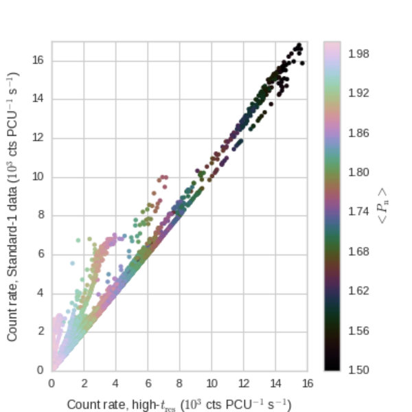 Figure 1
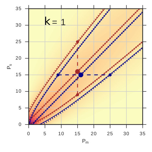 Figure 2
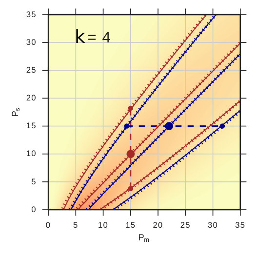 Figure 3
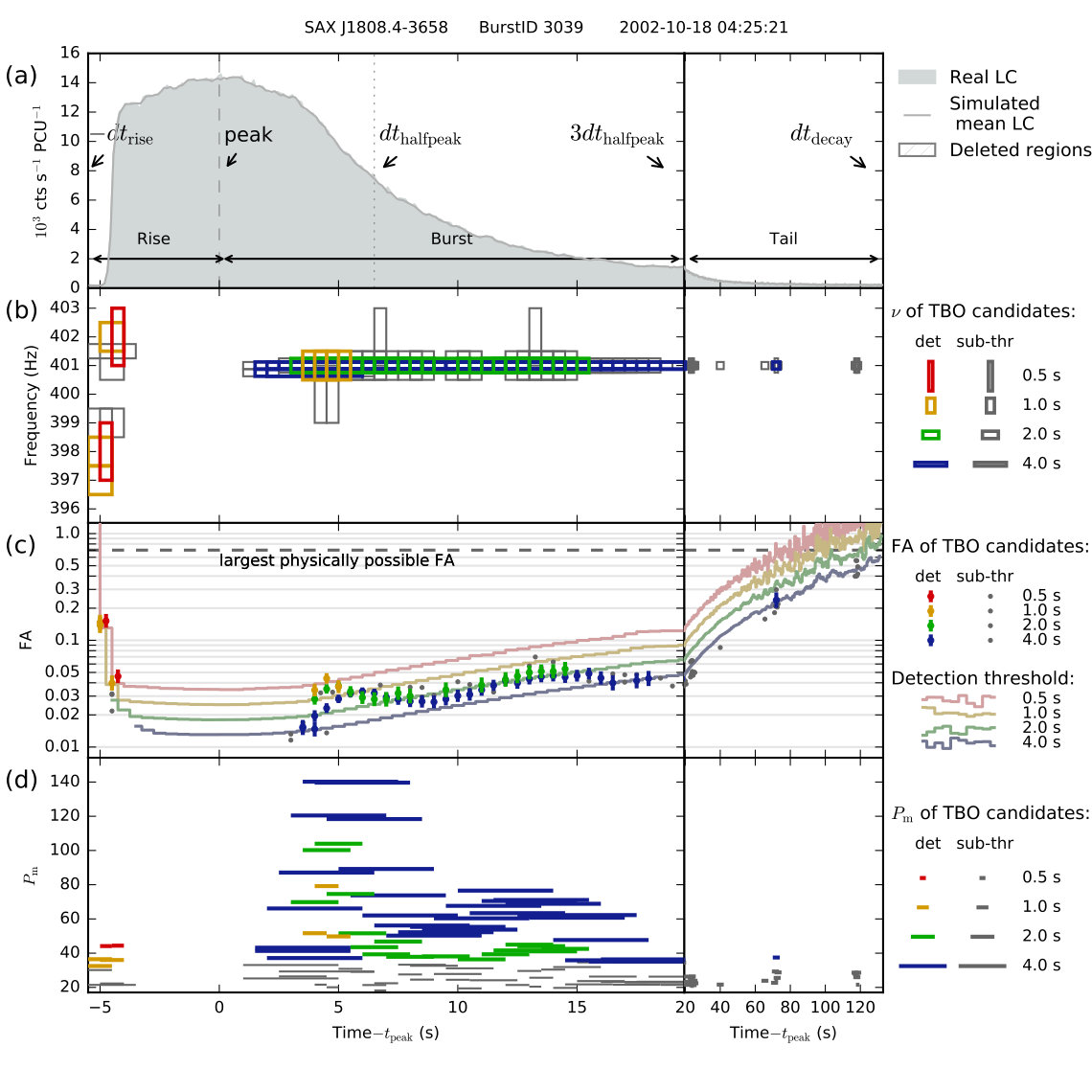 Figure 4
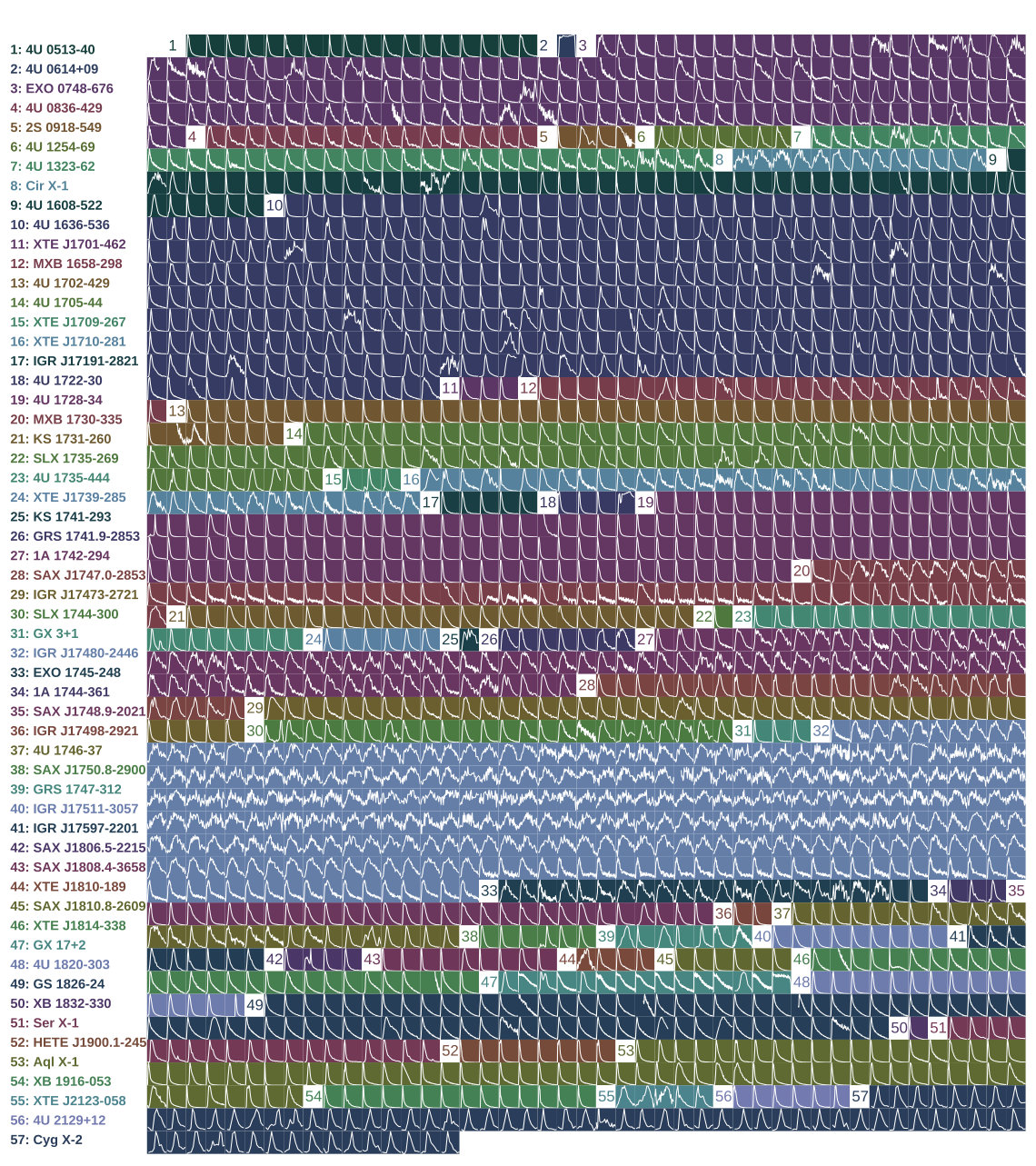 Figure 5
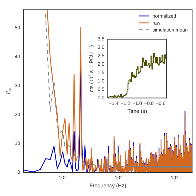 Figure 6
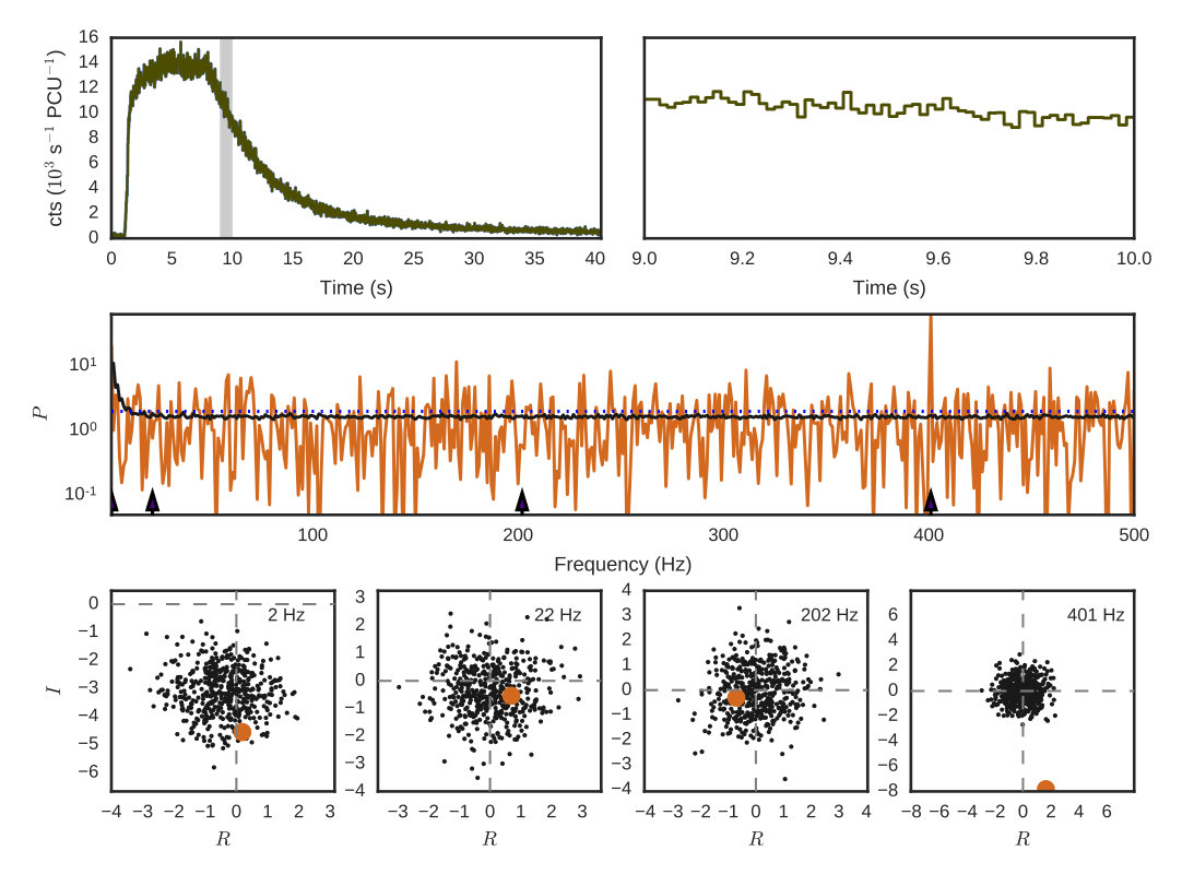 Figure 7
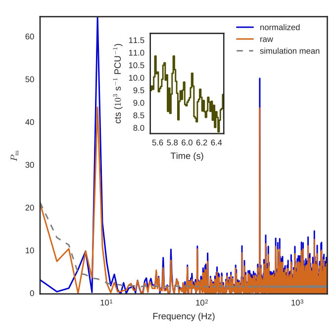 Figure 8
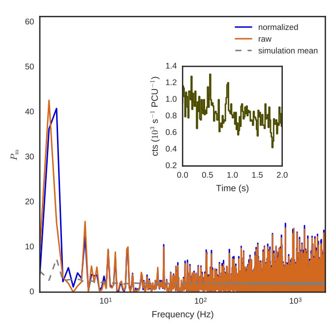 Figure 9
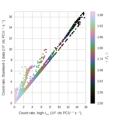 Figure 10
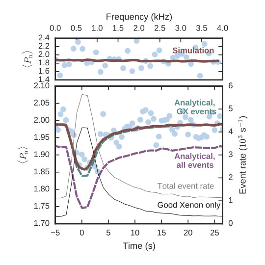 Figure 11
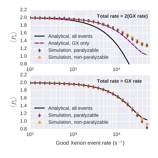 Figure 12
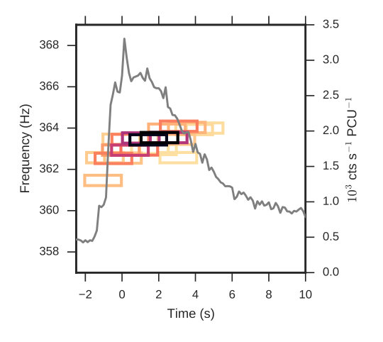 Figure 13
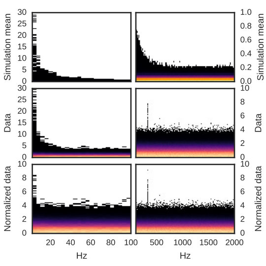 Figure 14
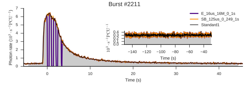 Figure 15
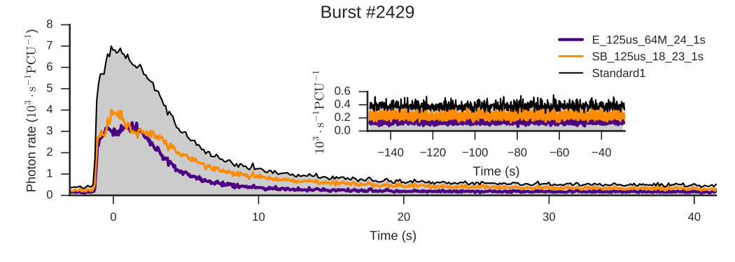 Figure 16
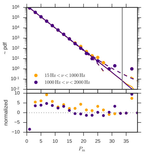 Figure 17
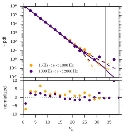 Figure 18
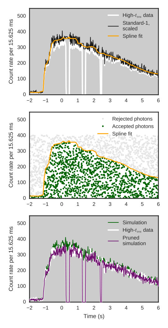 Figure 19
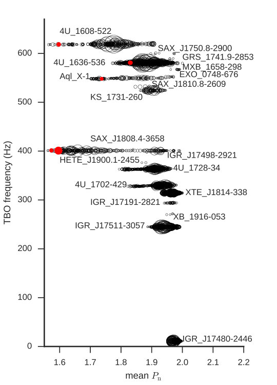 Figure 20
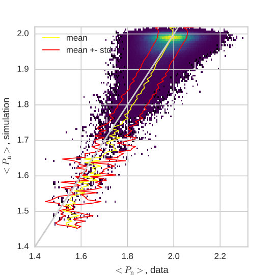 Figure 21
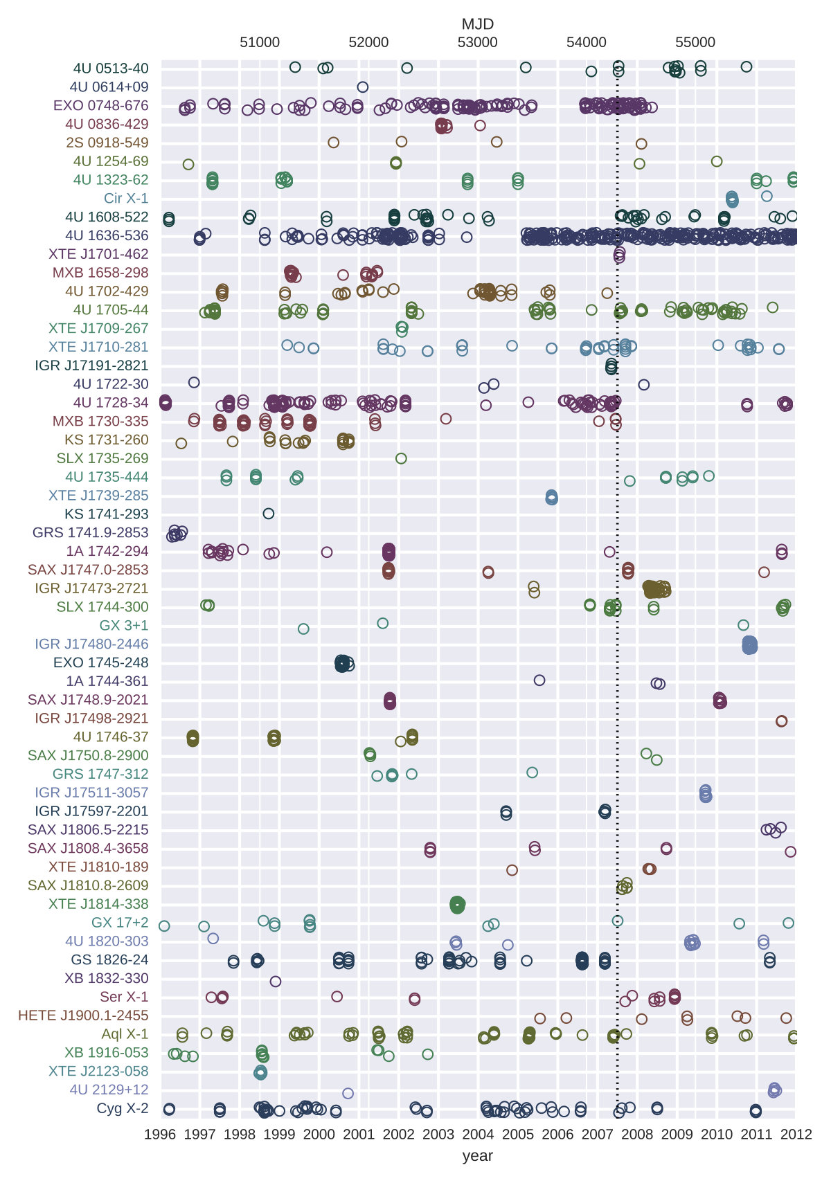 Figure 22
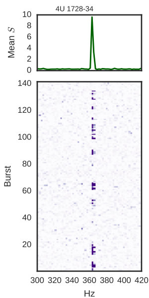 Figure 23
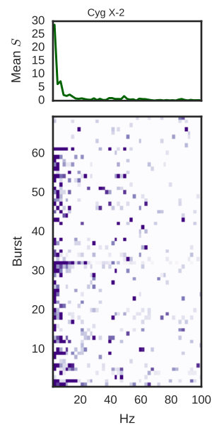 Figure 24
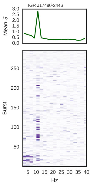 Figure 25
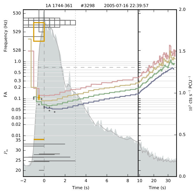 Figure 26
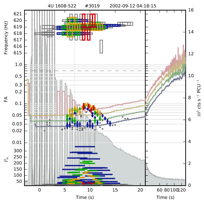 Figure 27
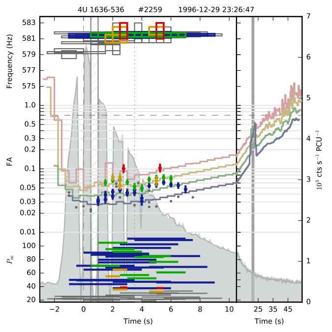 Figure 28
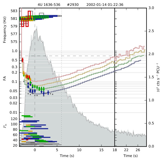 Figure 29
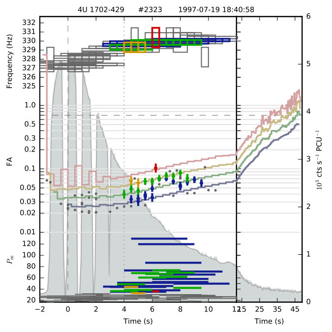 Figure 30
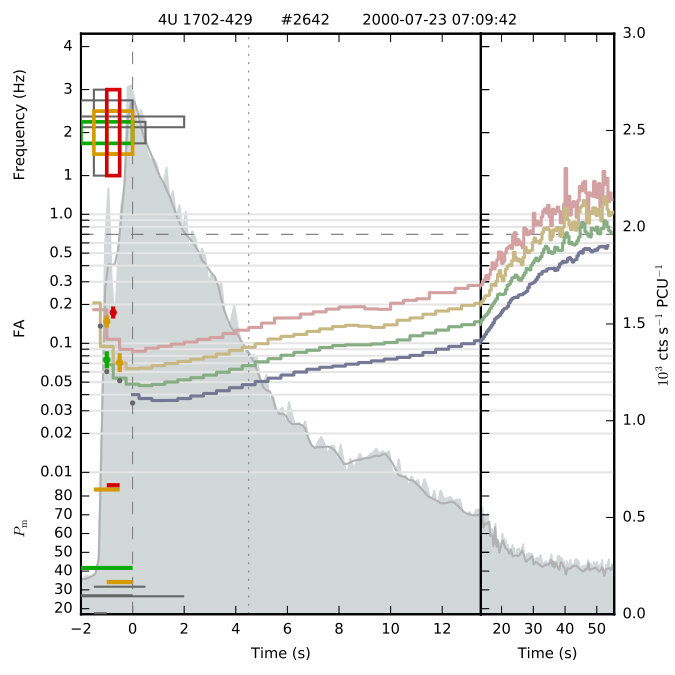 Figure 31
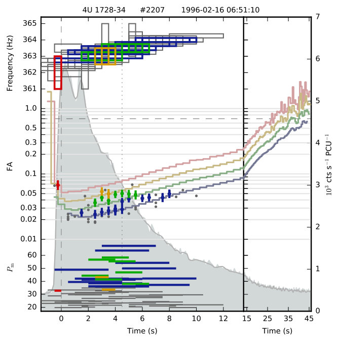 Figure 32
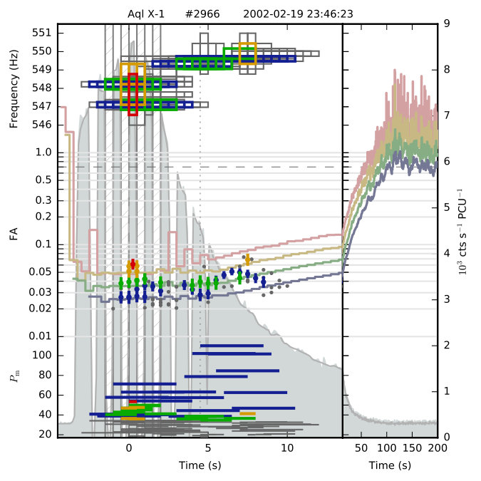 Figure 33
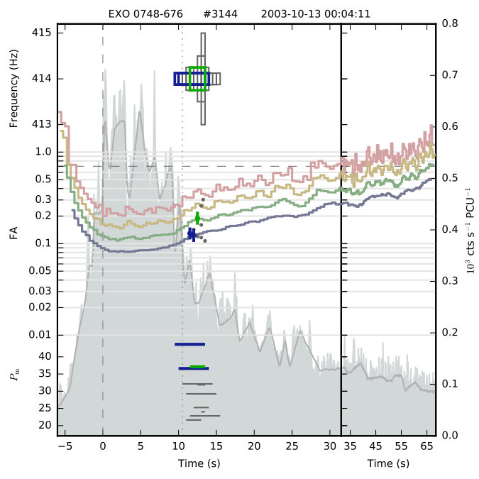 Figure 34
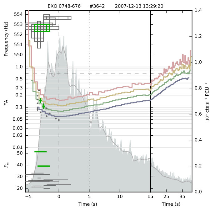 Figure 35
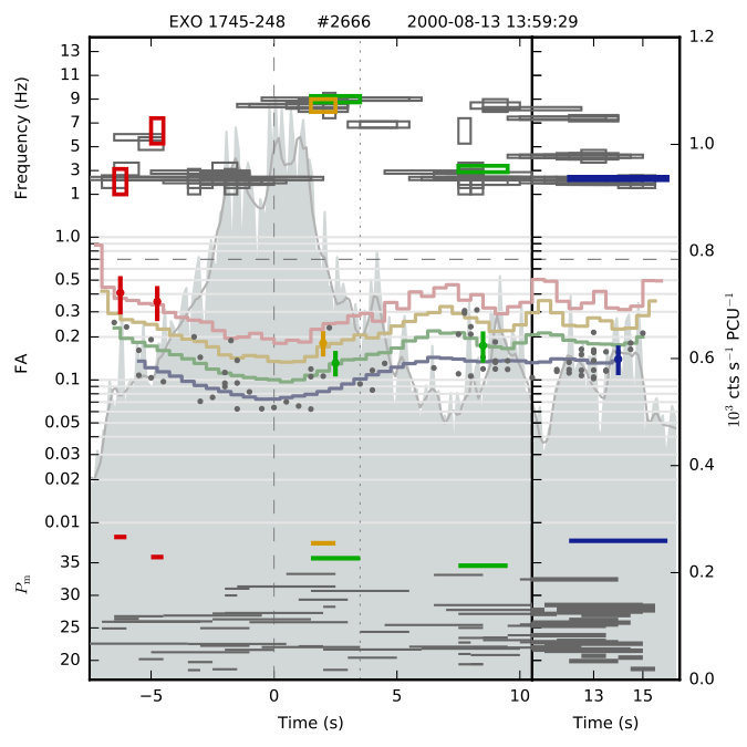 Figure 36
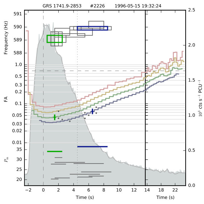 Figure 37
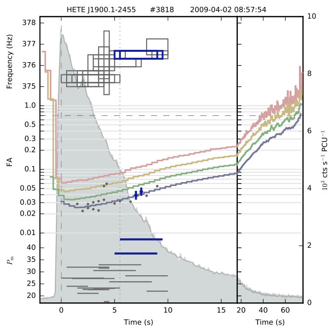 Figure 38
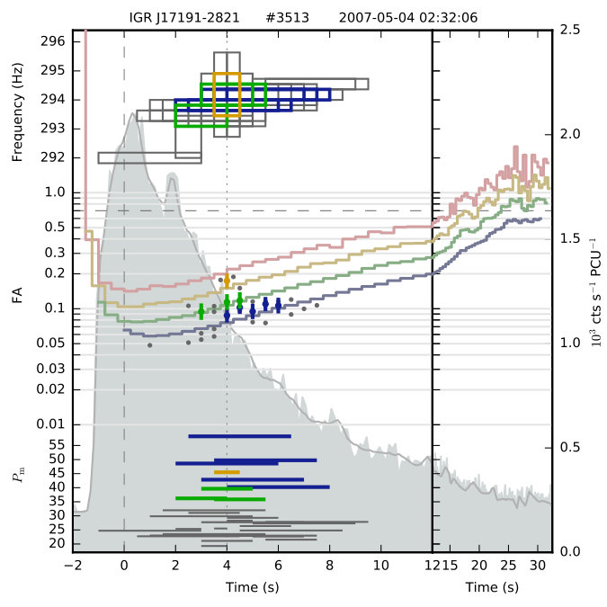 Figure 39
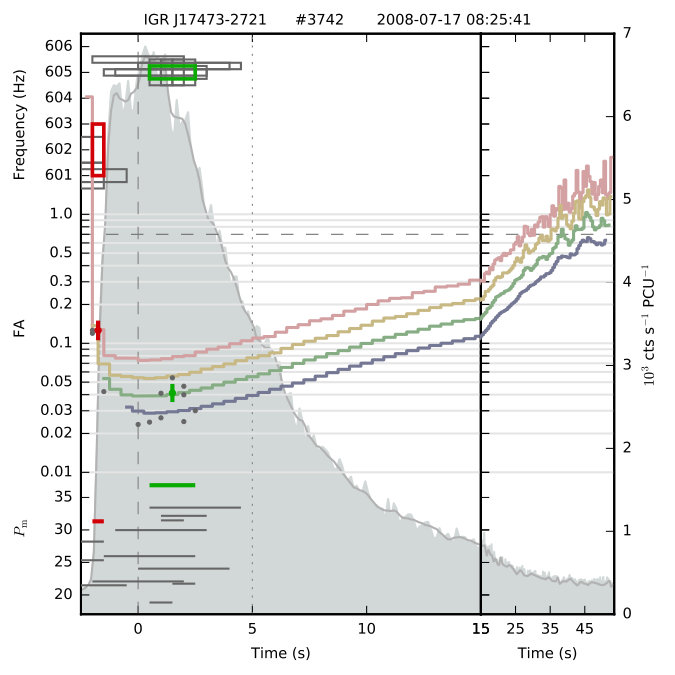 Figure 40
| given | given | |
|---|---|---|
| Median | ||
| Mean | ||
| Standard deviation |
| 1 | 2 | 3 | 4 | 5 | 6 | 7 | 8 | 9 | 10 | 11 | 12 | 13 | 14a | 14b | 14c | 14d | ||
|---|---|---|---|---|---|---|---|---|---|---|---|---|---|---|---|---|---|---|
| min (%) | ||||||||||||||||||
| Source | Entry | MINBAR TOA | (MET) | Rise (s) | Half-max (s) | Tail (s) | Peak S/N | Data mode | Notes | Max | 0.5 (s) | 1.0 (s) | 2.0 (s) | 4.0 (s) | ||||
| HETE J1900.12455 | 3301 | 2005-07-21 23:00:32 | 364604449.9 | 14.5 | 30.5 | 413.5 | 1607.7 | E_125us_64M_0_1s | gaps, bad LC, freq cov | 34.8 | 383.50 | 4.0 | 4.6 | 4.5 | 3.3 | 2.4 | ||
| 3362 | 2006-03-20 11:34:06 | 385472056.4 | 7.5 | 9.5 | 118.0 | 510.1 | SB_125us_8_249_1s | 29.2 | 228.00 | 4.0 | 4.6 | 3.3 | 2.4 | 1.7 | ||||
| 3667 | 2008-02-10 20:32:51 | 445293182.9 | 9.0 | 5.5 | 86.0 | 435.8 | E_125us_64M_0_1s | 35.2 | 12.00 | 0.5 | 7.2 | 5.2 | 3.8 | 2.7 | ||||
| 3818 | 2009-04-02 08:57:54 | 481280277.9 | 2.0 | 5.5 | 76.0 | 729.4 | SB_125us_8_249_1s | 43.5 | 376.25 | 4.0 | 6.1 | 4.5 | 3.3 | 2.5 | ||||
| 3820 | 2009-04-04 19:06:51 | 481489619.9 | 6.0 | 3.5 | 97.0 | 777.7 | E_125us_64M_0_1s | 28.5 | 1471.00 | 2.0 | 6.6 | 4.8 | 3.5 | 2.6 | ||||
| 3944 | 2010-07-07 21:04:32 | 521154292.9 | 12.0 | 6.5 | 118.5 | 672.8 | E_125us_64M_0_1s | 32.6 | 674.50 | 2.0 | 7.1 | 5.2 | 3.8 | 2.7 | ||||
| 3960 | 2010-09-20 05:29:04 | 527578164.4 | 7.5 | 8.5 | 92.0 | 427.1 | SB_125us_8_249_1s | 27.6 | 1313.50 | 4.0 | 6.0 | 4.3 | 3.1 | 2.3 | ||||
| 8257 | 2011-09-29 23:43:46 | 559957439.4 | 7.5 | 5.0 | 74.5 | 554.3 | E_125us_64M_0_1s | 30.3 | 776.00 | 4.0 | 7.0 | 5.1 | 3.7 | 2.8 | ||||
Peer Reviews
No public reviews on file for this paper yet. If you reviewed it on a platform where reviews are public (OpenReview, ICLR, NeurIPS, ICML), you can paste yours below so the community can read it here.
Videos
No videos yet. Explain this paper in a talk, walkthrough, or lecture? Add one.
A uniform search for thermonuclear burst oscillations in the RXTE legacy dataset
Anna V. Bilous
Anna L. Watts
Anton Pannekoek Institute for Astronomy, University of Amsterdam, Science Park 904, 1098 XH Amsterdam
Abstract
We describe a blind uniform search for thermonuclear burst oscillations (TBOs) in the majority of Type-I bursts observed by RXTE (2118 bursts from 57 neutron stars). We examined 2–2002 Hz power spectra from the Fourier transform in sliding 0.5–2 s windows, using fine-binned light curves in 2-60 keV energy range. The significance of the oscillation candidates was assessed by simulations which took into account light curve variations, dead time and sliding time windows. Some of our sources exhibited multi-frequency variability at Hz that cannot be readily removed with light-curve modeling and may have an astrophysical (non-TBO) nature. Overall, we found that the number and strength of potential candidates depends strongly on the parameters of the search. We found candidates from all previously known RXTE TBO sources, with pulsations that had been detected at similar frequencies in multiple independent time windows, and discovered TBOs from SAX J1810.82658. We could not confirm most previously-reported tentative TBO detections or identify any obvious candidates just below the detection threshold at similar frequencies in multiple bursts. We computed fractional amplitudes of all TBO candidates and placed upper limits on non-detections. Finally, for a few sources we noted small excess of candidates with powers comparable to fainter TBOs, but appearing in single independent time windows at random frequencies. At least some of these candidates may be noise spikes that appear interesting due to selection effects. The potential presence of such candidates calls for extra caution if claiming single-window TBO detections.
burst oscillations; LMXB
††journal: ApJS
1 Introduction
Thermonuclear burst oscillations (TBOs) are fast (typically, with a frequency of a few hundreds of Hz), relatively faint (fractional amplitude of a few percent) oscillations of photon count rate, detected in about 20% of known Type I X-ray bursts111http://www.sron.nl/~jeanz/bursterlist.html, see also Galloway et al. (2008), Watts (2012), and references therein.. The phenomenon of TBOs is attributed to the development of bright patches during thermonuclear explosions on the surface of accreting neutron stars. Several theories of patch formation have been proposed: flame spreading from the ignition point of the bursts (e.g. Strohmayer et al., 1997b), cooling wakes (Mahmoodifar & Strohmayer, 2016), convective patterns (Garcia et al., 2018), or large-scale (magneto)hydrodynamical oscillations in the burning material, induced by the spreading flame (e.g. Heyl, 2004). However, none of them can explain all of the observed TBO properties, motivating the development of better physical models for the ignition and progression of thermonuclear reactions on the neutron star surface (see the review by Watts 2012).
From the observational side, it is important to establish as complete a picture of TBOs as possible. Finding TBOs and constraining their properties is not always straightforward: although oscillations are highly coherent, their frequencies can drift (or jump) by a few Hz during the typical few-second duration of the TBO, with oscillations sometimes disappearing and reappearing throughout the burst (Muno et al., 2002a, b). The standard TBO search method relies on the Fourier transform (or calculation of -statistics) in a series of closely overlapping windows covering the burst duration (e.g. Strohmayer et al., 1998). Blind searches assume a constant frequency within a single time window, since searching for frequency derivatives adds an extra dimension to parameter space and is thus computationally expensive.
Estimates of signal significance are traditionally done analytically, based on simple photon counting statistics (Groth, 1975; van der Klis, 1989). At the same time, it has been recognized that the distribution of noise powers in real spectra is more complicated, being influenced by the burst envelope and dead time of the detector (van der Klis, 1989; Zhang et al., 1995). Using overlapping time windows and custom data filters complicates calculations of the number of independent trials, and thus estimates of TBO candidate significance. Some previous studies addressed these issues by discarding low frequencies affected by variation of the photon count rate due to the burst envelope (e.g. Ootes et al., 2017), directly measuring the dead time-affected average noise power (e.g. Thompson et al., 2005), using a conservative number of trials (e.g. Bhattacharyya, 2007), or estimating candidate significance with the simulation of data for a small number of bursts (e.g. Kaaret et al., 2007).
Searching for TBOs requires a sensitive instrument, operating in hard (1–30 keV) X-rays and capable of providing s time resolution. So far, the majority of TBO studies have been performed using the large set of observations from the Rossi X-ray Timing Explorer (RXTE, Jahoda et al., 2006), although other telescopes such as Swift (Strohmayer et al., 2008) and AstroSat (Verdhan Chauhan et al., 2017) have also been used to search for TBOs. The relatively quiet period that followed the termination of RXTE’s mission in Dec 2011 ended with the recent launch of NICER (Arzoumanian et al., 2014) in 2017; and ongoing studies for the next generation of instruments, such as eXTP (Zhang et al., 2019) and STROBE-X (Ray et al., 2018), are also providing new impetus for TBO studies.
Previous TBO searches explored relatively small subsets of data and were conducted using different methods or search parameters. In order to prepare for searches with new satellites and to provide a uniform picture for theoretical modeling of TBOs, we have undertaken the first comprehensive blind search for TBOs across almost the entire archival RXTE burst data set, using the 2015 pre-release version of the Multi-INstrument Burst ARchive (MINBAR222https://burst.sci.monash.edu/minbar/, Galloway et al., in prep). We use the standard approach of constant frequency and overlapping windows, but estimate the significance of candidates through data simulation that takes into account lightcurve (LC) variations, dead time and number of trials. This more realistic noise model allows us to search for TBOs in the regions of parameter space that were omitted or poorly examined before, such as low TBO frequencies ( Hz) or TBOs at very high count rates. We also search for clusters of candidates just below our detection threshold. We pay special attention to bursts with reported TBO candidates, which were afterwards deemed as tentative or controversial, and prepare our own list of potentially interesting candidates for subsequent follow-up with upcoming missions. Finally, the obtained frequencies and fractional amplitudes of TBOs or the upper limits on FAs of non-detections will provide important input for the TBO mechanisms (see e.g. Heyl (2004) and Piro & Bildsten 2005).
2 Significance estimate of PS for idealized light curves
Burst oscillations are very coherent pulsations which typically last for several seconds. During this time the oscillation frequency may jump or drift by several Hz. The search for TBOs is therefore usually conducted in separate, but often heavily overlapping time windows of about 0.25–5 s. Within each window, the photon arrival times are binned into sub-ms bins, then the Fast Fourier Transform (FFT) is taken from the number of photons versus time and the obtained power spectrum (PS) is examined for outliers. An example of such spectrum is shown in Fig. 1. An alternative to a FFT PS is to use statistics (Buccheri et al., 1983), which do not require binning of photon arrival times, and can be computed on a finer grid of frequencies (including variable frequency). statistics are more computationally expensive than FFTs, so they are usually used to search for TBOs from sources with known oscillations in a narrow range of frequencies (e.g. Watts et al., 2005).
2.1 Probability of false detection and the distribution of intrinsic signal power
Once the PS has been computed, potential oscillation candidates are identified as harmonics exceeding a certain threshold. Two questions immediately emerge: (a) for a given candidate, what is the probability of obtaining this power purely due to noise fluctuations, and (b) given the recorded power, what is the distribution of true signal power? The answers to both questions were given in the work of Groth (1975). Below, we repeat the author’s derivations in a somewhat modified form, using a different (nowadays, standard) normalization for the power spectrum.
In Groth (1975) the data time series is assumed to be composed of signal and noise:
[TABLE]
where is the number of photons in a given time bin and the subscripts correspond to measurement (m), signal (s) and noise (n). The coefficients of the Fourier transform of , for real and for imaginary, are the sum of the corresponding coefficients for signal and noise:
[TABLE]
If has a Poisson distribution, then both and have normal distributions. For the so-called Leahy-normalized (Leahy et al., 1983):
[TABLE]
normal distributions are standard, with mean of 0 and variance of 1. In this case will have a distribution with 2 degrees of freedom.
Assuming that the signal is deterministic, Groth derived an analytical expression for the joint probability distribution of the measured power and the signal of power :
[TABLE]
where in this equation is a modified Bessel function of the first kind and is the number of PS samples summed. Here, both and are Leahy-normalized and the whole derivation is valid if the total number of noise photons in the time window, , is larger than approximately ten.
Eq. 4 can be used to estimate the probability distribution of as a function of the measured power , , or alternatively the probability distribution of measured power as a function of the signal power , . Fig. 2 shows an example of the 2D probability density for and , together with the median and percentiles for and .
Table 1 gives expressions for the median, mean and standard deviation of 1-D distributions and . The mean and standard deviation of were given in Groth (1975) and are exact. The rest of the moments are useful approximations, obtained using numerically computed values for and both and smaller than 200. For , the approximations are valid when . For these the absolute value of discrepancies between the approximation and the numerically computed moments are , and , for the median, mean, and standard deviation, respectively. For , the median value deviates from by for .
For , Eq. 4 expresses the probability of obtaining without any signal, due to noise alone. This is used to estimate the significance of a potential signal detection. For , Eq. 4 reduces to:
[TABLE]
which is the probability density function (pdf) for the distribution with two degrees of freedom. It can be also shown that for the pdf is the distribution with degrees of freedom.
2.2 Fractional amplitudes
Besides oscillation frequency, power spectra contain information about the amplitude of pulsations. For example, for a Leahy-normalized PS, the rms fractional amplitude (FA) is defined as:
[TABLE]
Let us show that for the simplest case of a purely sinusoidal wave on a constant-rate background, described by a measured photon count of , the fractional amplitude calculated from Eq. 6 is, on average, equal to . In this specific case the noise count rate is described by the Poisson process with a mean rate of , and the signal is . The Leahy-normalized power spectrum of the signal is, by definition:
[TABLE]
Here, the average total number of noise photons is equal to its average rate times the number of time bins: . Since , . For a sine wave with amplitude , scipy DFT333https://docs.scipy.org/doc/numpy-1.13.0/reference/routines.fft.html yields PS harmonic with an amplitude of . Thus, the Leahy-normalized and .
In the limit of very small noise, approaches . However, formal calculation of fractional amplitudes may result in arbitrarily large . If there is no signal present, , , and is distributed as with degrees of freedom. The formally estimated given observed , regardless of its actual probability, yields a median value of (Table 1). For sufficiently large , can be such that .
Rms fractional amplitude is not a uniformly accepted way of describing oscillation amplitude. Some authors quote a full fractional amplitude () or a half fractional amplitude ().
For the actual burst observations, the noise level has a contribution from background unrelated to the observed low-mass X-ray binary (both astrophysical and instrumental), and the persistent emission from the source itself. The fractional amplitudes are usually calculated for photons in the burst only:
[TABLE]
with being an estimate of the number of background photons collected during the burst interval.
While analyzing fractional amplitudes one should bear in mind that there may be additional complications biasing the obtained values: the persistent emission may increase during the burst (Worpel et al., 2013, 2015) and there may be pulsed background, unrelated to TBOs, such as accretion-powered pulsations (APPs) or a pulsed reflection component from the accretion disk.
2.3 Complications and caveats
The standard approach described above provides a simple and relatively fast method for searching for TBOs. However, there exist some complications and caveats:
(a): The burst count rate may vary significantly within the typical time window (e.g. during the burst rise). This results in excess power at low frequencies, and biases estimates of and its significance.
(b): Because of dead time (time during which the detector is busy processing the current event and cannot record the next one), noise statistics deviate from . The influence of dead time is larger at higher count rates.
(c): Searching for TBOs in overlapping windows complicates the assessment of the number of independent trials, and thus the significance of .
(d): Abrupt variations of the burst count rate cause covariance between harmonics in the PS spectra. This may create the illusion of rapid drift or splitting of the TBO frequency.
In the following sections we are going to address caveats (a)-(c), complementing the traditional approach with more realistic noise modeling. The influence of rapid count variation on the recorded TBO frequency will be explored in a subsequent work (Bilous & Watts, in prep).
3 RXTE data set
The observations were performed in 1996–2011 with the proportional counter array (PCA, Jahoda et al., 1996) on board the RXTE telescope. The PCA consists of five identical co-aligned proportional counter units (PCUs), each with a circular field of view. The number of active PCUs varied between observing sessions and over the course of RXTE’s mission two PCUs went out of order permanently444https://heasarc.gsfc.nasa.gov/docs/xte/recipes/stdprod_guide.html. The PCA is sensitive to photons in the energy range between 2 and 60 keV. Photon counts are processed independently by up to six Event Analyzers (EAs). Two EAs record data in the standard modes, namely Standard-1 ( s, one energy channel) and Standard-2 ( s, 128 energy channels). The rest of the EAs can be configured in a variety of modes, representing the trade-off between time and spectral resolution due to finite data transfer capacities while streaming the data from the satellite to Earth.
Incoming photons can be recorded in two data modes: either with all photon arrival times recorded separately (“Science Event” mode) or with arrival times binned in small time bins (“Science Array” mode). Typically, Science Event files have good spectral resolution, but suffer from data losses at high count rates. Those Science Array files, which have the bin size suitable for oscillation analysis, usually have little information about photon energies, but are less prone to data losses. Often, the data were recorded in both Scientific Event and Scientific Array modes and sometimes different time resolutions and energy cuts are available for a single observation.
Burst selection was based on the information available in the 2015 pre-release version of the MINBAR database, which contains the times of arrival, source associations and other properties of Type I bursts observed with different satellites. We selected all bursts observed with RXTE, excluding bursts which: (a) did not have high- ( ms) data during the burst and either immediately before or after the burst (b) did not pass the extended good time interval (GTI) criterion555https://heasarc.gsfc.nasa.gov/docs/xte/abc/data_files.html (c) were missing spacecraft housekeeping data, or (d) had variable bin size in Scientific Array mode. The final sample contained 2118 bursts from 57 sources666We omitted two known RXTE superbursts (in’t Zand, 2017).. In this work we use the MINBAR catalogue burst entry number as a unique burst identifier.
For this paper we did not include Burst Catcher data, which can be also used for TBO searches (Zhang et al., 1998; Kaaret et al., 2002). This omission was not crucial as there were no bursts that were missing high time-resolution data on the burst rise, or throughout the burst, that would have been covered by the relevant Burst Catcher mode (the one with time resolution of 500 s or less). Nevertheless, several bursts with severe data gaps may benefit from the use of burst catcher data (e.g. burst #2266 from Aql X-1, see also Zhang et al. 1998).
For each of the 2118 bursts, we downloaded the data for the observations777legacy.gsfc.nasa.gov covering the MINBAR burst arrival time. We made a reference light curve, using the Standard-1 data re-binned to 0.5 s and searched for a LC peak within min of the MINBAR burst arrival time. The peak time served as the absolute reference point within each burst. LCs were visually inspected and the baseline window was selected manually for each burst. For most of the bursts the baseline window lay within (, ) s, but often it was placed in the burst tail (if no pre-burst data were available) or was shorter because of observation duration constraints or the presence of other bursts nearby. The on-burst window, (, ), was confined to the region where photon count exceeded the baseline mean plus two of its standard deviations. The on-burst window was manually adjusted for bursts with peculiar shapes and faint bursts. Figure 3 shows an example of LCs, the baseline and on-burst windows for two bursts from 4U 172834, recorded in different data modes.
In the event that more than one high- data mode was available for a single burst, we selected files with the largest number of photons per on-burst window, fewer gaps or with finer time resolution. We did not discard any photons based on their energy, and merged together data files which covered parts of the energy band (e.g. SB_250_us_0_13_2s and SB_250_us_14_35_2s). Sometimes files recorded in different data modes contained completely the same information; in this case the data mode was chosen arbitrarily. For uniformity, we converted Scientific Array files to the pseudo-Scientific Event format by recording the counts in each time bin as individual photons with time of arrival equal to the bin start time.
Photon arrival times were converted from the Mission Elapsed Time (MET) seconds to the UTC time system with the TIMEZERO value. This leads to timing accuracy888https://heasarc.gsfc.nasa.gov/docs/xte/abc/time.html of 100 s, which is sufficient for searching for burst oscillations in small windows (up to 4 s) if one is not trying to phase-connect oscillations between different bursts. Since the noise modeling relies on the housekeeping data that provides information at regularly sampled time intervals in the MET, in this work we chose not to barycenter the data.
Appendix A provides more detailed information about the burst sample. Two overview figures show burst times of arrival, source-by-source (Fig. 17) and Standard-1 LCs (Fig. 18). Table A available in its entirety in machine-readable form lists entry # and burst arrival time from MINBAR, in MET, rise, half-peak and decay times, S/N of the burst peak, data mode and notes for each burst. Notes indicate manual windows for faint bursts and bursts with peculiar shapes, presence of data gaps, partial GTI coverage or incomplete burst coverage.
4 Noise simulation and data analysis
In order to estimate the significance of oscillation candidates, for each burst we created a number of artificial oscillation-free bursts, which followed the properties of real data as closely as possible. The same search analysis was then conducted on real and simulated data.
Originally, we simulated the bursts by scrambling the intervals between photon arrival times in s windows. The size of the window was chosen to be much larger than the presumed TBO period, but smaller than the timescales of most large-scale LC variations. A similar technique was used by Fox et al. (2001), however the authors scrambled the LC bins, not the time intervals between individual photons.
Such scrambling preserves deviations from the noise distribution, but destroys any oscillation signal. However, it appeared that this method failed to produce enough statistically independent realizations of noise for some of the count rates. Statistical independence was assessed in the following way: we generated a sequence of 100 photons with constant rate and random arrival times, then reshuffled the time differences between them 1000 times, and computed the power spectra. For each harmonic, the Kolmogorov-Smirnov test was performed to test whether the 1000 realizations were consistent with being drawn from a distribution. For about 45% of cases the -value was smaller than , indicating large deviations from . Acceptable -values were obtained only for a number of photons larger than about 10000.
Thus, the scrambling method was abandoned. Instead, we performed random generation of photon time of arrivals (TOAs) using the approximated LC, with subsequent pruning according to known dead time.
4.1 Light curve modeling and simulation of photon TOA
RXTE records four types of events: “Good Xenon Events” (events which pass all of the discriminators and anti-coincidence vetoes, the desired astrophysical signal) and three types of events considered to be mostly due to instrumental background: “Coincidence Events”, “Very Large Events”, or “Propane Events” (Jahoda et al., 2006). “Good Xenon” events are recorded per PCU; for the rest the sum over all active PCUs is saved. All four types of events were simulated, since all of them cause dead time, influencing the number of recorded Good Xenon events.
In order to simulate the arrival times we used the information from the Standard-1 files, which contain events from the whole energy band, binned in 0.125 s bins. Sometimes, this binning is not sufficient for characterizing the burst rise properly. We therefore re-normalized the Standard-1 LC999Namely, Good Xenon and Propane Coincidence LCs. The Very Large Event LC was not renormalized because its count rate is usually low and does not change much during the burst. with the weights obtained from the higher- data, binned to 1/8 of the Standard-1 resolution (15.625 ms), keeping the total number of Standard-1 events in 0.125 s bins unchanged. If the higher- data were unavailable due to data gaps, uniform weights were applied (Fig. 4, top). LC count rates were adjusted for the dead time (see more details in Sect. 4.2).
We followed two different procedures for simulating Good Xenon events and the instrumental background. For the Good Xenon events we used a method which was more expensive computationally, but which resulted in better reproduction of the stochastic variation of the count rate.
The method was as follows. First, the dead time-corrected LC was smoothed with a median filter with a typical length of 0.5 s and a linear spline fit was performed to obtain the estimate of the count rate in any arbitrary moment of time (Fig. 4, top). The tolerance of spline fit and the size of the median filter window were adjusted on a per-source basis, so that the fit was maximally smooth, yet preserved, by eye, the short-timescale variations in the LC shape. However, for frequencies below Hz it becomes complicated to distinguish between potential TBOs and non-TBO LC variation, so in this region spurious candidates may be present or the significance of TBO candidates may be underestimated (see discussion in Sect. 5). Light curves for each individual PCU were obtained by multiplying the spline fit by the total number of Standard-1 photons recorded by a given PCU, divided by the sum from all PCUs.
Then, the arrival times of the Good Xenon events were simulated for each PCU separately using the acceptance - rejection method (von Neumann, 1951). We used the standard Python random number generator based on the Mersene Twister algorithm (Matsumoto & Nishimura, 1998) to generate pairs of random variables . Here, is the maximum value of and is the number of 0.125-s time bins in the on-burst window (Fig. 4, middle). Both and were uniformly distributed within and the on-burst window, respectively. Then, the pairs with were discarded. This way, a Poisson distribution of photon TOAs was created, with the instantaneous rate closely matching , but devoid of any oscillations with periods smaller than the characteristic time scale of the features of the modeled burst envelopes.
For the Propane, Coincidence and Very Large events we used a simpler procedure. The light curve counts were divided by the number of PCUs, and for each time bin with local count rate we generated the following number of uniformly distributed TOAs:
[TABLE]
where floor denotes the floor function and Binom is a binomial random variable with number of trials and success probability . This way the number of simulated photons is very close to the real data value and thus the simulation does not emulate the Poisson noise which is present in the data.
4.2 Dead time pruning
Simulated events were subsequently pruned to account for the detector’s dead time. Dead time calculation for RXTE is rather complex and thus deserves a detailed examination. According to Jahoda et al. (2006), RXTE PCUs process events independently and the dead time is caused by all events recorded by the PCU. Any event recorded belongs to one and only to one of the four classes101010http://heasarc.nasa.gov/docs/xte/recipes/pca_deadtime.html: Good Xenon, Coincidence, Very Large, or Propane Events.
In general, there exist two types of dead time: paralyzable (cumulative), where events entering the detector during dead time themselves cause further dead time (even though they are not recorded); and non-paralyzable, where events entering detector during dead time are completely ignored. For RXTE, the actual dead time is a mixture of both types, depending also on event class and assigned energy. However, for most of cases can be approximated as 10 s non-paralyzable dead time (set by the analog-to-digital converter, ADC) for all classes except VL events. For VL events, the dead time can vary between 70 s and 500 s and depends on the instrumental setting, most of the time being approximately 170 s (Jahoda et al., 2006).
Zhang et al. (1995) developed an analytic formula for the Leahy-normalized noise PS in the presence of dead time. The mean value is always less than 2 by some amount which depends on event rate, the type of dead time and its value, the LC bin size, , and the FFT frequency. The analytic formula for paralyzable dead time has a much simpler form than that for the non-paralyzable dead time.
Jahoda et al. (2006) gives an example showing how to calculate the dead-time modifications to pure noise for a count rate below cts PCU*-1* s*-1*, applying the correction for the paralyzable dead time. Disregarding larger for the VL events:
[TABLE]
Here indicates noise (as in Sect. 2), is the output rate of all events (all four types combined), is the dead time, is the bin size, is the FFT frequency, is the number of frequencies in the PS, is the Nyquist frequency. The authors also give an ad hoc correction for the larger of VL events, which is much smaller than the one introduced by Eq. 10 for our and and VL event rates.
Although technically RXTE dead time is a complex mixture of both paralyzable and non-paralyzable dead times, with the non-paralyzable dead time of ADC contributing the most at energies below keV, for the typical RXTE rates and size used in this work, the formulas for paralyzable and non-paralyzable dead times yield essentially the same corrections. Thus, the more simple Eq. 10 can be used to estimate the dead time influence on the average noise power.
For our simulations, we treated dead time as purely non-paralyzable. Note that we do not model the absence of dead time caused by events which triggered only or alpha chains. According to Jahoda et al. (2006), not doing this leads to a small overestimation of dead time fraction by , an amount nearly constant throughout the mission.
Fig. 5 shows the average signal power in Burst #2980 from Aql X-1 (in which no TBOs were detected). Photons from only one PCU were selected, and a bin size of s was used, together with an FFT window of 1 s. For this choice of binning and the rates of Good Xenon (GX) and other events the noise power has only a minuscule dependence on FFT frequency. We have summed all harmonics above 10 Hz (below 10 Hz the PS may be affected by red noise) and compared the noise power to the mean obtained from 1000 simulations, which appeared to match the data well (Fig. 5).
Attempting to apply Eq. 10 yielded interesting results: if the rate was taken to be the rate of all events (since all of them cause dead time), as stated in Jahoda et al. (2006), the dead time correction was considerably and consistently larger than that required to match both data and simulations. However the correction did match observations well if only the GX events were taken into account. It appears that for the given range of event rates and the bin/dead time windows, the operations of dead time pruning and selection of GX events are commutative, meaning that GX photons have the same noise power distribution as if they were not affected by the dead time from all other event types. As simulations have shown, this does not hold true for larger count rates (Fig. 6), however, such large count rates do not occur in our burst sample.
To summarize, dead time was accounted for in the following way: initially LC curves for all four event types were re-normalized using the fraction of dead time calculated with the observed rates111111The RXTE Cook Book states that ”the VLE rate is not affected by dead time”, this was not reproduced in the simulations.. Then the TOAs of the four types of events were simulated separately and combined to form a “mixed-bag” event sequence which mimicked the real data. Then events which arrived within 10 s after previous non-VL event and variable after VL event were removed. Those events were assumed not to cause dead time themselves, so the dead time was by definition non-paralyzable. This procedure was performed for each PCU separately, and then the resulting photon lists were merged together.
4.3 Accounting for data gaps and occasional limited energy range
Data gaps are losses of data due to saturated telemetry occurring for bursts with high count rate. They typically last from a fraction of a second to several seconds and are not reflected in the Good Time Interval table of the data files. To search for data gaps, we selected all time intervals with gaps between two successive photons being larger than 0.02 s. In order to exclude “natural” gaps in bursts with intrinsically low count rate, we calculated the estimated number of photons inside the potential gap and selected only those gaps where this number was larger than two. The number of photons inside the gap was estimated from the mean photon count rate of Standard-1 data and adjusted for the overall difference in the energy band (multiplied by a sum of all Standard-1 counts divided by the sum of all high- counts for the time bins where the latter was larger than 0). All simulated photons inside the data gaps were deleted.
Finally, the photon sequences were adjusted for the difference in energy band between high- data and the Standard-1 data (e.g. Fig. 3). For each 0.125-s bin, the ratio between Standard-1 LC and the high- data LC was estimated and the simulated data were pruned by deleting the appropriate fraction of photons at random (Fig. 4, bottom).
Both real and simulated photon sequences were binned with sub-ms time bins. For observations in Good Xenon data mode, the bin size was , yielding about 8 phase bins in pulse profile at the highest frequency searched. For all other modes, the bin size was two times larger, corresponding to the typical s. Although 24 bursts had larger , they were still binned with the smaller bin size. Among those bursts, five had , all of them from GRS 1747312. For these bursts any candidates at frequencies above the Nyquist frequency of 1024 Hz were discarded.
4.4 Fourier transform
Fourier transforms were taken for the binned sequences in series of 0.5, 1, 2 and 4-s sliding windows, each window starting 0.5 s later than the previous one. The FFT coefficients and were recorded for harmonics between 2 and 2002 Hz. The lower limit was set by the smallest non-zero harmonic for the PS in 0.5 s windows. The upper limit reflects the largest possible NS spin frequency allowed by current reasonable models of the neutron star equation of state (Haensel et al., 2009).
In what follows, we will operate with FFT coefficients in a cell, with being the FFT frequency, referring to the center of the time window and being the given window size. The 500 simulation runs were used to make distributions of and in each cell. The and had, most of the time, Gaussian distributions with the mean influenced by the baseline variation and the standard deviation influenced by the dead time (Fig. 7). We used the mean and unbiased estimate of standard deviation of the first simulation runs to normalize and of the real data. Power spectra from the remaining 100 runs, normalized as the same way as the real data, were used to estimate detection significance.
The mean and standard deviation and used for re-normalizing are inevitably influenced by the limited number of simulation runs. For pure Poisson noise, the means are random variables with normal distribution, having and . Since , the standard deviation is also distributed normally, with and . Since the dead time influence has negligible dependence on Fourier frequency, for the normalization we averaged the standard deviation by harmonics in order to reduce the stochastic error caused by the limited number of simulations. Simulation of pairs of standard normal random variables showed that re-normalizing them by the mean and standard deviation drawn from the appropriate Gaussian distributions causes about 10% of detections above the threshold set by (adopted as the detection criterion, see Sect. 4.5) to be false positives. Another 10% of un-normalized candidates had power below the threshold after normalization. It is hard to estimate the rate of false negatives or false positives for the real-data candidates, since it depends on the intrinsic distribution of TBO powers. However, we checked the normalization values for all candidates that were deemed interesting, for example occurring in an unusual place in the burst or being detected from a burst without previously reported TBOs.
In rare cases of a gap occupying most of the FFT window, and become covariant at the lowest Fourier frequencies. In such cases the subsequent analysis is not applicable, so we discarded candidates from those cells. The covariance threshold was estimated as follows: we simulated 500 independent normal random variables and the distribution of covariance was calculated. The threshold was set as 5 times the standard deviation of the covariances.
We also checked for the covariance along the frequency axis. Such covariance stems from abrupt changes in photon count within the window, caused by data gaps or even on the burst rise if the latter is sharp. For each time window and simulation we calculated autocorrelation function (ACF) from the renormalized simulated . ACFs from all 500 simulations were added together and the 50% half-width of the peak was measured, with the baseline levels subtracted from the peak. We discarded PS in the given time window (regardless of frequency) if the 50% half-width of the ACF peak was larger than 5 harmonics. Such bursts were marked with “freq cov” comment in the notes column of Table A.
Finally, we removed the cells covering regions where the simulated LC deviated substantially from the real data due to narrow gaps or spikes. Substantial deviation was defined being larger than 10 standard deviations of the simulated photon count in given 0.125 s or 15.625 ms time bins. Such bursts were marked with “bad LC” comment in the notes column of Table A.
4.5 Filtering potential oscillation candidates and computing fractional amplitudes
In order to filter potential TBO candidates, we selected all cells with renormalized , where corresponded to a probability of getting chance candidates per single spectrum:
[TABLE]
The choice of was arbitrary and motivated by the requirement to have a manageable number of candidates for the given data sample. For 0.5, 1, 2 and 4-s FFT windows was 30.85, 32.24, 33.62, and 35.01, respectively. was adopted as the upper limit in the event that no candidate detections were found.
Since the power values in adjacent cells are covariant both in time and (to a smaller extent) in frequency, the number of trials is not equal to the number of cells, , and the simple significance formula is not readily applicable. To assess the significance of detections, we performed the same candidate search for the simulated data and compared the number of oscillation candidates from the real data with the distribution of the same values from the simulated data.
For each potential candidate we computed fractional amplitude (FA) using Eq. 8 and the median value of from Table 1, . The uncertainties in fractional amplitudes were calculated by linear error propagation of the independent parameters in Eq. 8 (Ootes et al., 2017). For the uncertainty on , we took [0.159, 0.841] percentiles of the distribution. The uncertainty on the number of photons in the FFT window was taken to be Poissonian and the uncertainty in the background level was taken to be the standard deviation of count rates in the baseline window, computed in the overlapping windows of the length equal to the current FFT window.
A few potential uncertainties are not included in the given FA errors. Firstly, we do not include the variation of background within the burst from Worpel et al. (2015), since it is not available for all bursts in our sample. We also do not correct for the possibility of the TBO frequency falling between FFT harmonics. Simulation showed that with our choice of FFT windows and oversampling in time, fractional amplitude can be underestimated by as much as a factor of 0.68. However only in 9% of cases (assuming no prior knowledge of TBO frequency) suppression of FAs is stronger than 0.85.
Finally, we did not account for bias caused by the limited number of trials. Simulated distribution of for the normalized data had a mean and median consistent with the ones from Table 1. The standard deviation of for the normalized data was larger by a small value of .
4.6 Organizing the results
Table A gives a general picture of the maximum power recorded for each individual burst, as well as the smallest FA of potential detection (defined by the threshold detection probability, Eq. 11). Besides renormalized power , it lists its frequency and , as well as smallest for all four .
Table A contains basic properties for each source (number of bursts, total duration, median S/N of the burst peak, minimum and median upper limits on FAs in 1-s window at the burst peak), providing an overview of the amount and quality of observational material for each source as well as the extent of FA range that can be probed by our analysis. The properties of oscillation candidates are given per frequency group, with a group being defined as the candidates with Hz (matching the lowest frequency resolution). For each frequency group we list the number of bursts with TBO candidates in this frequency range and the number of bursts with candidates in one of three non-overlapping regions: “R”, defined as the region between rise and peak of the burst; “B” starting at the peak and spanning three times half-peak width (more or less corresponding to the traditional on-burst windows); and “T” covering the rest of the burst tail. For each frequency group we list also the average of the candidates in each of the four Fourier windows. The remaining three columns give a handle on the number of spurious candidates in both real and simulated data, listing the total number of real-data non-TBO candidates (counting the ones from overlapping windows as independent and omitting low-frequency ones), the average number of candidates in the simulated data (averaged over 100 simulation runs) and the percentile of the real-data number with respect to a 100-run simulation sample, .
Table LABEL:table:det gives more detailed information about each group of candidates (except for the low-frequency ones) for each individual burst, listing MINBAR burst entry, MINBAR TOA, frequency range, location of candidates within the burst (R, B or T), number of independent time windows and the maximum FA for each size of Fourier window.
Finally, for each group of candidates we provide reference plots, aggregating information about frequency, time of arrival, power and FA of candidates, as well as upper limits on FAs. Fig. 8 gives an example of such a plot, with separate panels for the burst LC and the frequency, FA, and power of the candidates. To conserve space, the rest of the reference plots are made more condensed, without legends and with individual panels merged together.
5 Results
5.1 Low-frequency noise
The mean values of simulated Fourier coefficients, and , give us a handle on how much the power spectrum is affected by the change of photon count rate during Fourier window. Fig. 9 shows an example of the frequency-dependent distribution of the absolute values of Fourier coefficients for all cells in the bursts from 4U 1702429, omitting the cells with large frequency covariance or large discrepancy between the simulated and real LCs (see Sect. 4.4). At higher Fourier frequencies the spread of and is mostly determined by the finite number of simulation runs, whereas at the lower frequencies we record an excess of large coefficient values. For the majority of the sources this excess continues to at least 100 Hz. In rare cases the frequencies as high as 1000 Hz can be still affected.
Re-normalization of Fourier coefficients allowed us to remove most of the described power excess. However, we still record a relatively large number of strong candidates at frequencies below Hz. Some of these candidates can be associated with obvious flaws in LC modeling, where our spline failed to reproduce short peaks or drops in the LC (Fig. 10, left, hereafter “type I” low-frequency candidates). Other low-frequency candidates cannot be immediately connected to the imperfect LC modeling (hereafter “type II” low-frequency candidates). Several sources (e.g. Cyg X-2, EXO 074876, EXO 1745248) exhibited such unexplained bursts of low-frequency candidates spanning multiple harmonics and sometimes showing at distinctly separate frequencies (Fig. 10, right). The origin of this type II low frequency noise remains unclear: it could well be astrophysical, associated with either the bursting surface or the accretion disk (see for example van der Klis, 2006).
Although mostly recorded from fast-spinning neutron stars, TBOs can occur at frequencies as low as 11 Hz (IGR J174802446, Cavecchi et al., 2011). So far, only one such slow TBO source is known and finding another one (or the one spinning at even lower frequency) would be very interesting. In general, however, we found that power spectra at the lowest frequencies of few Hz are difficult to interpret, since it is hard to distinguish between LC variation and oscillations here. An example of such a problematic spectrum is shown in Fig. 11. Oscillations with a frequency of about 3 Hz are clearly visible in the lightcurve. With the given choice of smoothing and spline fitting parameters, LC modeling removes some of the count rate variation and changes the shape of the peak in the power spectrum. More stringent LC models can reproduce the observed LC variations, removing the peak completely
We have inspected visually all diagnostic plots featuring type II low-frequency candidates looking for signals resembling the 11 Hz TBOs from IGR J174802446: with detections in multiple independent time windows and multiple bursts, at frequencies larger than the lowest recorded frequency of 2 Hz and without candidates of comparable strength at the nearby, but distinctly separate frequencies. No such candidates were found.
5.2 Dead time
In Section 4.2 we reviewed the methods of estimating the influence of the instrument’s dead time on the observed noise statistic . In this section we will examine the from the whole set of observations in our sample.
In order to investigate the dead time influence, we recorded the mean non-normalized simulated power at frequencies above 1 kHz. At these frequencies the bias caused by LC variation is small for all of our sources (Sect. 5.1). We found that the simulated noise power did not have any discernible dependence on the number of PCUs that were on, and varied between 1.5 and 2, depending on the total photon count rate recorded by the PCUs (obtained from Standard-1 data files). This count rate is always equal to or larger than the count rate derived from the high- data.
Fig. 12 (left) provides the reference for average simulated noise power versus count rate per PCU in high- and Standard-1 files. For count rates larger than cts s*-1* PCU*-1*, is smaller than about 1.7, differing dramatically from the value of 2 prescribed by the ideal noise model. Thus, neglecting dead time influence for bright bursts can lead to an underestimation of the potential signal significance by orders of magnitude. The average power is considerably smaller than 1.7 at the peaks of at least one burst from 4U 061409, 4U 1608552, Aql X-1, HETE J1900.12455, and SAX J1808.43658.
Comparison of noise powers between real and simulated data is not straightforward because of the large intrinsic noise variance: for obeying distribution with two degrees of freedom, the standard deviation of noise powers is 2, the same as the mean value. Averaging all harmonics above 1 kHz reduces the standard deviation to for s and allows us to pinpoint the influence of dead time. For simulated data, additional averaging by 100 simulation runs further reduces the standard deviation by a factor of 10. Fig. 12 (right) shows the 2D distribution of such average noise powers in real and simulated data. For most values of simulated power, the noise powers for the real data appeared to be statistically slightly larger than the corresponding simulated power, most probably stemming from the simplifications we made during dead time pruning. The discrepancy can reach as much as 0.15 for , but is not larger than 0.02 for the more common . This leads to an overestimation of the real data candidate significance by a factor that can be as large as few (for the largest count rates), but more commonly of about a few percent.
It is worth mentioning that dead time also biases the measured fractional amplitudes of TBO candidates, since the fraction of dead time is different during the crests and troughs of the oscillation trains. Using non-normalized in Eq. 8 may bias FAs by as much as a factor of .
5.3 Overall simulation quality and glimmer candidates
In order to assess whether our simulations are adequately reproducing the data, we compared the distributions of normalized powers for the real and simulated data sets. For each source and we combined powers in two frequency regions: between 15 and 1000 Hz (thus, excluding any low-frequency noise), and between 1000 and 2000 Hz (see Fig. 13, left, for an example). The distributions for real data and the mean distribution of 100 simulation runs match reasonably well. Moreover the distribution of normalized is well described by statistics, assuming a conservative number of trials (i.e. treating all time windows as independent, Fig. 13, right). The same is true for the candidates from all four combined – the estimates of the average number of candidates using Eq. 5 and assuming all windows and harmonics to be independent are not dramatically different from the average number of candidates from the simulation runs (see also Table A).
However, for some of the sources the match is not perfect. After normalizing the real-data distribution by the corresponding mean and standard deviation of 100 simulated-data distributions, one can see that there is a systematic discrepancy between the two for . The amount of discrepancy is usually larger for frequencies below 1000 Hz and varies considerably from source to source. It may stem from imperfect dead time or LC modeling, or any weak broadband astrophysical signal.
For some of the sources, we found a small excess of higher-power candidates (e.g. with on Fig. 13). This excess can be present in either of the two frequency groups and is equivalent to 5–10 standard deviations in a given power bin. The examination of the cumulative versions of the normalized power distributions for all combined showed that for several sources, e.g. 4U 1608522, EXO 0748676, Cyg X-2, and others, the number of candidates above the detection threshold on the real data (excluding frequency ranges of known TBO) is larger than the corresponding number in % of the simulation runs (, see Table A). On the other hand, the prolific TBO source 4U 1636536 yielded fewer real-data noise candidates than any of 100 simulations. The origin of this discrepancy is unclear.
Such marginally significant noise candidates (dubbed “glimmer candidates”, reflecting potential attractiveness) are detected in a single independent time window, at seemingly random, never repeating frequencies121212Except for two 1108-Hz candidates from EXO 0748676, see Table A. and throughout all on-burst windows. Some of the candidates occur at lower frequencies in time windows with substantial count rate variation and their significance is very sensitive to LC modeling. Glimmer candidates can be present in the bursts with TBOs, sometimes even in the same time bins as TBOs. Folded glimmer candidates produce sinusoidal profiles and some of them are stronger than weak TBOs (e.g. Fig. 14).
It must be noted that whether the source has glimmer candidates depends on the detection threshold. For example SAX J1808.43658 has at standard detection threshold, however the power of some of the noise candidates is much larger than any of the simulated powers. On the other hand, for MXB 1658298 drops from 0.06 to 0.01 if the threshold probability is multiplied by 3.7 (Sect. B.1.4).
One must be very careful in interpreting glimmer candidates. By definition, the source has glimmer candidates if the number of detections outside TBO frequencies and not immediately connected to low-frequency noise is larger than the number of candidates in 99% of simulation runs. This means that assuming a sufficiently large number of bursts per source, 1% of all sources will have glimmer candidates purely due to chance. At our detection threshold, five sources, or 8.8% had , which is larger than the expected 1%, suggesting that at least some of the glimmer candidates may have an astrophysical origin. Some may for example be connected to type II low-frequency candidates which happen to occur at somewhat higher frequency and more than 2 Hz apart from other candidates, thus being placed in a separate frequency group by our grouping procedure.
5.4 TBOs from known oscillation sources
Seventeen TBO sources were known prior to our analysis. These are the sources with TBOs detected at similar frequencies, in several independent time bins, several bursts or at frequencies close to the frequency of APPs. All of these sources yielded candidates at the frequencies close to those reported previously and all but one had more candidates than any of the simulation runs () in a purely blind search. We note that the TBO candidates from the accreting MSP HETE J1900.12455 would not have been significant in our blind search which neglected closeness to the known APP frequency for this source, since the TBOs come from one independent time window and have moderate power. For the other sources, sometimes we did not have any candidates (including sub-threshold, see Sect. 5.8 for our definition of sub-threshold candidates) where they have been reported previously. This may be explained by differences in data processing.
In general, we find that the measured power of TBO candidates depends strongly on the size of the Fourier window and its location. Because we searched in several windows of different length, we were able to give a more complete picture of the fractional amplitudes, which may be important for bursts with more than one oscillation train, i.e. bursts with photospheric radius expansion (PRE), with a short train of TBOs in the rise and a longer train after the burst peak). We have compiled an extensive dataset of fractional amplitudes (Table LABEL:table:det) as well as upper limits for each of the four window lengths (Table A), to support future studies of TBO physics (see Sect. 6).
For many of the TBO sources a considerable fraction of TBO candidates came from the data regions with large influence from dead time (Fig. 15). Low-frequency noise does not have much of an influence – only in a few cases the absolute mean values of the simulated Fourier coefficients were larger than (see Sect. 4.4, 5.1 and Fig. 9). More information about each TBO source is given in Section B.1.
5.5 Tentative TBO detections from the literature
Eight sources in our sample had tentative TBO detections prior to our analysis (see Table 2 in Watts, 2012). Here we summarize the results of our analysis of these sources, more detailed information about each of them is given in Section B.2.
No TBO candidates were detected in the only burst from 4U 061409, observed by RXTE. Previously, the 415-Hz oscillations were reported from one burst observed with Swift. The FA limits from the RXTE burst are more stringent than the detection reported from the Swift, but as we know from other sources, TBOs are not consistently detectable in all bursts from a given source.
The previously reported 529-Hz TBO candidate from 1A 1744361 was also detected in our analysis, however it was too faint to be significant given the number of trials. The presence of sub-threshold candidates tracing out a small frequency drift argues in favour of this candidate being a genuine TBO, but a new detection is needed to confirm this.
TBO candidates from 4U 125469 (95 Hz), XTE J1739285 (1122 Hz), and SAX J1748.92021 (410 Hz), discovered in time windows with sizes similar to the range of used in this work were in our analysis not significant enough to pass the detection threshold. The sources did not have any clusters of sub-threshold candidates close to the reported frequencies. TBO from another two sources, MXB 1730335 (306 Hz) and GS 182624 (611 Hz) were claimed based on stacked power spectra. None of our candidates for these sources were close to the frequencies reported in the previous papers.
XB 1916053, with its pair of TBO candidates at frequencies 2 Hz apart remained controversial in our analysis. In addition to these two candidates, we detect four other strong candidates, all of them potentially due to type II low-frequency noise. None of the simulated data sets had as many candidates as the real data, whether or not one counted the 270-Hz candidates as a TBO. A more precise estimate of the significance of this signal should take into account frequency separation between the candidates; however this is outside the scope of this current work.
5.6 New TBO discoveries
One more TBO source has been discovered, SAX J1810.82609, yielding strong () 531-Hz oscillations in one independent time window (see Sect. B.3.4). The candidate power so strong that it has small probability assuming the most conservative number of trials (counting all harmonics and all time bins from the whole 57-source sample as independent). Full details of this discovery are reported in Bilous et al. (2018).
Besides that, we recorded an interesting pair of -Hz candidates from IGR J174732721 (see also Sect. B.3.3). These candidates were faint (), but came within 3 Hz from each other and framed the burst peak during a burst with PRE, showing typical features of TBOs from established TBO sources (e.g. SAX J1750.82900).
5.7 Other sources
Out of the remaining thirty sources in our sample that had no published record of TBOs prior to our study twenty-three were unremarkable, with the number of noise candidates reproduced well by simulations. Some of these sources also had low-frequency noise of type I or II. Seven more sources had a marginally significant number of candidates (albeit occurring at random frequencies), or stronger and more broadband low-frequency noise. More details can be found in Sect. B.3.
5.8 Subthreshold candidates
Even if an individual candidate has moderate power that is below our nominal threshold, a cluster of sub-threshold candidates in a relatively narrow frequency range may indicate the presence of TBOs. We performed a simple search for such a clustering of sub-threshold candidates by summing the powers of all candidates with:
[TABLE]
which corresponds to of 17.03, 18.42, 19.81, and 21.19 for of 0.52 s. The sums, , were additionally added in 2-, 4- or 8-Hz frequency bins and normalized by burst duration. The stacks of were then inspected visually for traces of power excess correlated in frequency.
Interestingly, for known TBO sources the bursts without TBO candidates did not necessarily yield sub-threshold candidates, with in the TBO frequency range being similar to at other frequencies (e.g. Fig. 16, left). Nevertheless, some of the known TBO sources did have sub-threshold TBO candidates, with the most prominent example being IGR J174802445. Only two bursts from this source have candidates at 10–11 Hz in Table A, but many more bursts have relatively large (Fig. 16, middle).
About half of sources in our sample exhibited low-frequency noise on stacks, sometimes extending to Hz. For Cyg X-2, this frequency region was particularly noisy with multiple sub-threshold candidates at random frequencies (Fig. 16, right).
None of the sources showed any obvious clustering of candidates at frequencies different from the frequencies of known TBOs. This was something of a surprise: we had anticipated that there would be sub-threshold candidates emerging from such a large data set. It also must be noted that, similarly to most TBO searches, our analysis does not include the effects of any potential smearing due to intrinsic TBO frequency drift and Doppler shifts due to the motion of the Earth and the binary orbit, all of which would reduce detectability.
6 Summary
In this work, we conducted a large-scale blind search for thermonuclear burst oscillations for the majority of type-I X-ray bursts observed by RXTE. In comparison to previous work, our analysis encompassed more sources, and probed potential signals on a range of time scales and further into burst tails, treating all sources in a uniform fashion.
In order to estimate the significance of selected oscillation candidates, we developed a more realistic noise model by simulating photon sequences with variable count rate which mimicked the real light curves and was affected by dead time. Fourier spectra from simulated sequences were used to renormalize the corresponding Fourier spectra from the real data and thus to remove the low-frequency noise due to variable count rate, and to restore the dead-time-affected average power.
Our noise model showed that abrupt LC variations, for example during the burst rise or data gaps, can bias the noise statistics in a frequency-dependent manner at frequencies up to approximately 100 Hz, or, in several cases, even up to 1 kHz (thus, not being confined to low frequencies any more). LC modeling allowed us to remove most of this bias. However, in some cases we still detect strong candidates below 16 Hz. These low-frequency candidates did not immediately resemble known low-frequency TBOs from IGR J174802446: with detections in multiple independent time windows and multiple bursts, at frequencies larger than the lowest recorded frequency of 2 Hz and without candidates of comparable strength at the nearby, but distinctly separate frequencies. Some of the detected low-frequency candidates are clearly generated by single, poorly modeled sharp peaks or dips in LCs, these we refer to as “type I” low-frequency candidates.
Several more sources yielded candidates not immediately connected to flaws in LC modeling (e.g. Cyg X-2, 4U 172934, EXO 0748676, EXO 1745248, and others). Such candidates, dubbed “type II” low frequency candidates, frequently appeared to be grouped in time and/or frequency, sometimes appearing at distinct frequencies simultaneously. It is possible that these type II low frequency candidates may have an astrophysical origin: perhaps a non-TBO process on the burning surface, or varying emission due to the effect of the burst on the accretion flow (see for example Worpel et al., 2013, 2015). Generally, the signal at the lowest frequencies in our spectra (below approximately 5 Hz) is quite hard to interpret, since its strength depends substantially on how closely the model LC follows the real one.
The instrumental dead time had, somewhat surprisingly, a rather large influence on the power spectra statistics, with the average noise power dropping below 1.7 for the burst peaks of five sources, some of them with TBOs. Neglecting the influence of dead time can lead to underestimation of candidate TBO significance by as much as two orders of magnitude.
Overall, our noise models provide an important insight into the statistics of RXTE power spectra, but they do not give a perfect description of the data, most probably because of the set of assumptions regarding the dead time influence and what constitutes a “real” LC. Also, some bias is caused by the limited number of simulations run to derive the statistical properties of noise. From the computational point of view, it is much easier to estimate the average noise power using harmonics past kHz, renormalize the power spectra and use probability distribution with conservative number of trials (treating all time windows as independent, regardless of overlap) to estimate the candidate significance. However, this approach would not work at lower Fourier frequencies during the burst rise or during data gaps.
We have also found that abrupt changes in the LC rate (sharp rise or a data gap) can lead to covariance between adjacent Fourier harmonics and can manifest as a fast change of TBO frequency. A quantitative investigation of this phenomenon will be presented in subsequent work. Overall, data gaps obliterate part of the signal and bias the fractional amplitude evolution: using data with gaps should be avoided if at all possible. Future X-ray telescopes aiming to study this phenomenon should aim for high throughput.
For our study, we have selected all candidates with renormalized probabilities less than per spectrum. This resulted in the power thresholds varying with time window size. Our choice of detection threshold was to some degree arbitrary, but was motivated by a wish to analyze a manageable number of candidates. The significance of these candidate detections was then estimated by comparing the number of candidates in the real data to a pool of an additional 100 of simulated spectra, renormalized in the same way as the real data.
Our candidates included all previously known TBOs. For one of the sources, the accreting MSP HETE J1900.12455, the detection in a single time window was not significant because of the large number of trials in our analysis. The study that reported this finding originally searched a narrower frequency range around the known pulsar frequency (Watts et al., 2009). We find that the power of candidates depends dramatically on the specific window sizes and degrees of overlap used.
Overall, we have compiled an extensive data set containing information on the frequency and fractional amplitudes of all selected candidates, as well as upper limits on fractional amplitudes derived from the threshold powers. We anticipate that this information will be a valuable resource for future studies of TBO properties, particularly when used in conjunction with the burst property database MINBAR. The conditions under which TBOs are excited and detectable are important factors in assessing the viability of physical models for the TBO mechanism (Watts, 2012).
Eight sources in our dataset had prior claims of TBOs where the claimed detections were either weak and came from one independent time window (or, in the case of XB 1916053, two close but separated frequencies) in a single burst or several stacked bursts. We were unable to confirm TBOs from any of those sources. Some of the previously claimed detections had smaller powers in our analysis (which can be sensitive to the choice of the time windows) and were not significant when compared to noise simulations. For 4U 061409 we had different bursts than the ones with potential TBOs (which came from a different telescope); the burst in the RXTE sample showed no TBO candidates. Other claimed detections were based on analysis of stacked spectra and yielded no candidates in our time windows.
One of the sources without previously reported TBOs, SAX J1810.8-269 yielded a strong, brief 531-Hz pulsation in one of the bursts. The signal was detected in one independent time window, however its strength () speaks in favour of it being a TBO (for more in-depth significance analysis, see Bilous et al., 2018). The other sources did not provide any compelling TBO candidates, despite our removing most of the low-frequency noise and making better significance estimates for bright bursts. In addition, we found no groups of sub-threshold candidates, probing probabilities up to 100 higher than our adopted detection threshold. This was somewhat surprising: we had anticipated finding at least some clusters of sub-threshold candidates in such a large burst sample.
An interesting (albeit not formally significant in our analysis) pair of -Hz TBO candidates was recorded from IGR J174732721. The candidates were rather faint, but came close in frequency (within 3 Hz) and framed the burst peak during a burst with PRE. More than half of the simulation runs had as many or more candidates (at arbitrary frequencies) with at least the same significance.
Another source with previously-reported potential TBOs with similar characteristics, XB 1916053 had much more significant candidates, with as few as 2% of the simulations runs having the candidates at least as strong as the strongest one on the real data. Overall, IGR J174732721 and XB 1916053 would be interesting sources for subsequent follow-up.
Our estimate of candidate significance treated all frequencies as independent and did not include important TBO features such as frequency drift coupled with signal disappearance during PRE. In the case of weaker signals, it is currently unclear how small a gap in frequency should be for the signals to be attributed to a single TBO.
We have found that some of the sources exhibited a marginally significant number of noise candidates, meaning that 99% or more simulations runs had a smaller number of candidates. These candidates appeared at random frequencies both below and above 1 kHz in single independent time windows and were often stronger than some of the TBO detections in individual bursts, reaching . We dub them glimmer candidates. It is possible that some of the glimmer candidates are of astrophysical origin (especially the ones at lower frequencies).
7 Conclusions
TBOs are transient phenomena with rapidly changing properties. The measured power of potential TBO candidates depends greatly on the specific choices regarding data selection, such as energy filters, time windows, degree of overlap, summing harmonics or adjacent time windows and stacking spectra from different bursts. Thus, considering the researcher’s natural desire to find TBOs, one must be very careful with estimating the number of trials resulting from tweaking the search parameters and exploring multiple sources.
While searching for high-power narrowband signals using Fourier transform in overlapping time windows, it is generally reasonable to use a model of the distribution of the noise powers with the conservative number of trials, after correcting for dead time influence, LC variation and making sure that the harmonics in Fourier spectra are not covariant. However, it is strongly advisable to verify that a distribution actually describes well the noise powers of a given dataset.
Our search for TBOs resulted in several short (each detected in one independent time window) candidates with powers comparable to those of the fainter TBOs (). These candidates, dubbed “glimmer” are marginally significant, meaning that 99% or more simulations runs had a smaller number of candidates. They produce sinusoidal oscillation profiles and are in all aspects resembling fainter TBOs. However, they occur at random frequencies within a single source and sometimes are coincident in time with real TBOs. Partly, glimmer candidates may stem from selection bias, however an astrophysical origin is not excluded. Regardless of their nature, the phenomenon of glimmer candidates may explain the large number of unconfirmed single-window detections, e.g Kaaret et al. (2002), especially considering the tendency of underestimating the number of trials.
For the potential detections with the smaller power, the best corroboration of TBO nature is detecting the signal at the same frequency in independent time windows; however with the intrinsic frequency drift and Doppler modulations complicate it. It is therefore important to develop a procedure for estimating significance of signals with drifting or jumping signal. This would help refining the significance of frequency jump in MXB 1658298 (Wijnands et al., 2001), drifting candidate in 1A 1744361 (Bhattacharyya et al., 2006), a pair of 270-Hz candidates XB 1916053 (Galloway et al., 2001) and potential pair of 600-Hz candidates from IGR 17473 (this work).
Despite our efforts, we did not find TBOs below 200 Hz and during high count rates. Several measures can be undertaken in order to obtain a better, more complete picture of TBOs. Obtaining new data using better instrumentation with higher throughput leads to better sensitivity and the absence of data gaps allows a better characterization of the frequency evolution. Continuing searching is also an option, since TBOs may appear from the sources without promising candidates, although having some theoretical guidance would be better, something the data could be used for. Further improvement of TBO searches can also be made by selecting only that part of energy spectrum where there are most burst photons, in order to minimize the relative contribution of background. Having ephemerides would also help to correct for the Doppler change in frequency: this would be especially helpful for the ultra-compact binaries such as 4U 1820303 or the potential ultra-compact binary 2S 0918549.
A.V.B. and A.L.W. acknowledge support from ERC Starting grant No. 639217 CSINEUTRON- STAR (PI: A.L. Watts). We would like to thank Duncan Galloway and the MINBAR team for sharing a pre-release version of the MINBAR database with us. A.V.B. thanks Hauke Worpel for sharing the data on background variation during type I bursts.
Appendix A Times of arrival, light curves, and tables
\startlongtable
The reference list from the paper itself. Each links out to its DOI / PubMed record.
- 1Altamirano et al. (2008) Altamirano, D., Casella, P., Patruno, A., Wijnands, R., & van der Klis, M. 2008, Ap J, 674, L 45
- 2Altamirano et al. (2010 a) Altamirano, D., Watts, A., Linares, M., et al. 2010 a, MNRAS, 409, 1136
- 3Altamirano et al. (2010 b) Altamirano, D., Linares, M., Patruno, A., et al. 2010 b, MNRAS, 401, 223
- 4Arzoumanian et al. (2014) Arzoumanian, Z., Gendreau, K. C., Baker, C. L., et al. 2014, in Proc. SPIE, Vol. 9144, Space Telescopes and Instrumentation 2014: Ultraviolet to Gamma Ray, 914420
- 5Barrière et al. (2015) Barrière, N. M., Krivonos, R., Tomsick, J. A., et al. 2015, Ap J, 799, 123
- 6Bhattacharyya (2007) Bhattacharyya, S. 2007, MNRAS, 377, 198
- 7Bhattacharyya & Strohmayer (2006) Bhattacharyya, S., & Strohmayer, T. E. 2006, Ap J, 642, L 161
- 8Bhattacharyya & Strohmayer (2007) —. 2007, Ap J, 656, 414