Quantum cosmology in the light of quantum mechanics
Salvador J. Robles-P\'erez

TL;DR
This paper explores the analogy between universe evolution and particle trajectories, extending it to quantum mechanics, and introduces a super-field approach for multiverse states, offering new insights into quantum cosmology and spacetime quantisation.
Contribution
It presents a novel super-field framework for quantum cosmology, applying third quantisation to the multiverse and linking quantum states to spacetime geodesics and uncertainties.
Findings
Super-field propagates in minisuperspace representing multiverse states
Third quantisation parallels second quantisation of matter fields
Quantum uncertainties relate to spacetime geodesics
Abstract
There is a formal analogy between the evolution of the universe, when this is seen as a trajectory in the minisuperspace, and the worldline followed by a test particle in a curved spacetime. The analogy can be extended to the quantum realm, where the trajectories are transformed into wave functions that give us the probabilities of finding the universe or the particle in a given point of their respective spaces: the spacetime in the case of the particle and the minisuperspace in the case of the universe. The wave function of the spacetime and the matter fields, all together, can then be seen as a super-field that propagates in the minisuperspace and the so-called third quantisation procedure can be applied in a parallel way as the second quantisation procedure is performed with a matter field that propagates in the spacetime. The super-field can thus be interpreted as made up of…
Click any figure to enlarge with its caption.
 Figure 1
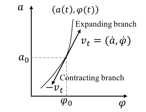 Figure 2
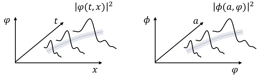 Figure 3
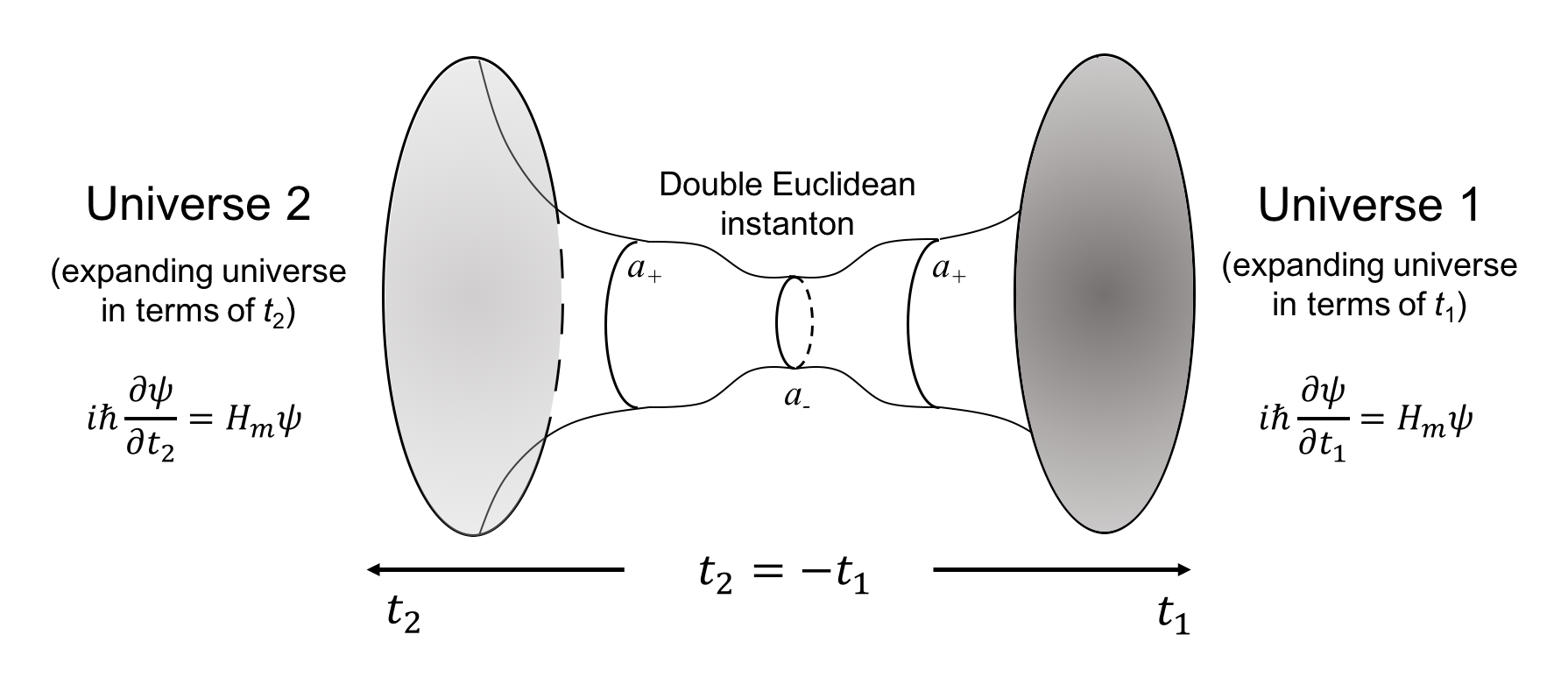 Figure 4
Peer Reviews
No public reviews on file for this paper yet. If you reviewed it on a platform where reviews are public (OpenReview, ICLR, NeurIPS, ICML), you can paste yours below so the community can read it here.
Videos
No videos yet. Explain this paper in a talk, walkthrough, or lecture? Add one.
Quantum cosmology in the light of quantum mechanics
Salvador J. Robles-Pérez
Estación Ecológica de Biocosmología, Pedro de Alvarado, 14, 06411 Medellín, Spain.
Departamento de matemáticas, IES Miguel Delibes, Miguel Hernández 2, 28991 Torrejón de la Calzada, Spain.
Abstract
There is a formal analogy between the evolution of the universe, when this is seen as a trajectory in the minisuperspace, and the worldline followed by a test particle in a curved spacetime. The analogy can be extended to the quantum realm, where the trajectories are transformed into wave functions that give us the probabilities of finding the universe or the particle in a given point of their respective spaces: the spacetime in the case of the particle and the minisuperspace in the case of the universe. The wave function of the spacetime and the matter fields, all together, can then be seen as a super-field that propagates in the minisuperspace and the so-called third quantisation procedure can be applied in a parallel way as the second quantisation procedure is performed with a matter field that propagates in the spacetime. The super-field can thus be interpreted as made up of universes propagating, i.e. evolving, in the minisuperspace. The corresponding Fock space for the quantum state of the multiverse is then presented. The analogy can also be used in the opposite direction. The way in which the semiclassical state of the universe is obtained in quantum cosmology from the quantum state of the universe allows us to obtain, from the quantum state of a field that propagates in the spacetime, the geodesics of the underlying spacetime as well as their quantum uncertainties or dispersions. This might settle a new starting point for a different quantisation of the spacetime coordinates.
pacs:
98.80.Qc, 03.65.−w
Contents
-
V.1 Semiclassical universes: classical spacetime and quantum matter fields
-
V.2 Semiclassical particles: geodesics and uncertainties in the position
I Introduction
In 1990 M. Gell-Mann and J. B. Hartle presented the sum-over-histories formulation of quantum cosmology in a paper entitled ”Quantum mechanics in the light of quantum cosmology”, in which the classical domains of familiar experience are derived from a decoherence process between the alternative histories of the universe. In that paper Gell-Mann and Hartle (1990), the authors conclude that quantum mechanics is best and most fundamentally understood in the context of quantum cosmology. This is so for many different reasons. First, the non-locality or, generally speaking, the non-separability of the quantum theory leads to the assumption that it cannot be applied only to a given system since it is not isolated but coupled to its natural environment, which is again coupled to another environment, and so forth Kiefer (1994). The extrapolation of that idea inevitably implies that the quantum theory must be applied, from the most fundamental level, to the universe as a whole. If this is so, then, the quantum mechanics of particles and fields must be a derivable consequence of the application of the quantum theory to the whole universe.
For instance, there is no preferred time variable in the universe so, strictly speaking, it cannot undergo any time evolution. However, we know from experience that the spacetime and the things that are deployed in the spacetime evolve in time. Therefore, as Gell-Mann and Hartle show, time and time evolution, and particularly the Schrödinger equation that provides us with the time evolution of quantum systems, must be emergent features of the quantum state of the universe. It is from that point of view from which the principles of quantum mechanics can be most fundamentally understood in the context of quantum cosmology, as the authors say. Furthermore, the universe jeopardises some of the fundamentals of the quantum theory. For instance, what does it mean concepts like uncertainty or non-locality in the context of a universe that is not deployed in the spacetime but it contains it? Thus, quantum cosmology forces us to acquire a deeper and a wider understanding of the quantum theory.
The idea behind quantum cosmology is that the conditions imposed on the state of the universe at the boundary111Time is created at the onset of the universe and thus the wave function of the universe cannot be a time-dependent function, so we cannot apply an initial condition on the state of the universe. However, the universe may have a boundary where to impose the conditions that eventually would determine everything else in the whole history of the universe., together with the equations of quantum mechanics should be enough to assign probabilities to any plausible event that may happen in the universe. This is in principle the most that a non deterministic theory like the quantum mechanics can provide. With that purpose, and following a parallelism with the Feynman’s formalism of path integrals, Gell-Mann and Hartle extend the seminal idea of Everett Everett (1957) and develop their sum-over-histories theory Gell-Mann and Hartle (1990, 1993); Hartle (1995), in which a history is defined as a time ordered sequence of projectors that represent all the possible outcomes that the infinite constituents of the universe may give at each moment of time222These are essentially the relative states of Everett’s formulation of quantum mechanics Everett (1957). However, Everett did not provide an explanation of why some states and no others are selected from the whole set of possible states. In order to explain it Hartle needs to add, besides the boundary condition of the state of the universe and the equations of quantum mechanics, a new ingredient: the coarse-graining process that makes some states to emerge from the decoherence process. These are the selected states of the Everett’s formulation.. These fine-grained histories represent therefore all the possibilities in the universe and, hence, they contain all the information of the universe. However, these histories interfere among each other so in order to assign independent probabilities to the exclusive outcomes of the semiclassical experience333The outcomes of a classical experiment are exclusive, i.e. the cat is either dead or alive but not both. one must take some coarse graining around the representatives values of the distinguished variables under study. In that process the fine detailed information is lost but it is because the loss of that ignored information that we can assign consistent probabilities to the alternative outcomes of a given experiment. It may seem then curious that the acceptance of a bit of ignorance is what allows us to obtain information from a physical system.
In the case of quantum cosmology, it turns out that (classical) time and the time evolution of matter fields, which constitute the main ingredients of the semiclassical domain of our everyday experience, are emergent features that decohere from the fine-detailed description of the quantum state of the universe Hartle (1995). Thus, the sum-over-histories framework provides us with a consistent assignation of probabilities to the different outcomes of a given experiment and, in cosmology, it supplies us with an explanation for the appearance of the semiclassical domains of everyday experience444The existence of a semiclassical domain in the universe, and actually our own existence, can be seen as two possible outcomes of the cosmological experiment. As Hartle says Hartle (1995), we live in the middle of this particular experiment., where it is developed the quantum field theories of matter fields; so, at least from the conceptual point of view, everything seemed to be settled in quantum cosmology. The idea that was left is that little else could be done. In order to understand quantum mechanically the primordial singularity we need a complete quantum theory of gravity, and short after the origin the inflationary process seems to blur any posible imprint of the quantum regime of the universe. Besides, everything that follows could be explained by the quantum mechanics of particles and fields that, in the light of quantum cosmology, are emergent features of the quantum state of the whole universe. Thus, quantum cosmology got stuck in the 90’s555Two important exceptions are the developments made in loop quantum cosmology Rovelli (2000) and the computation of next order gravitational corrections to the Schrödinger equation made in Refs. Kiefer and Singh (1991); Kiefer and Krämer (2012); Brizuela et al. (2016a, b). .
Almost thirty years afterwards, the title of this paper becomes a humble tribute to Gell-Mann and Hartle, and to many other authors that made possible the development of quantum cosmology Wheeler (1957); De Witt (1967); Hawking (1982, 1984a, 1984b, 1987); Vilenkin (1982, 1984, 1986, 1988, 1994, 1995); Hartle and Hawking (1983); Hartle (1990, 1995); Halliwell and Hawking (1985); Halliwell (1987, 1989, 1990); Kiefer (1987, 1992, 1994, 2007); Gell-Mann and Hartle (1990); Wiltshire (1996), and particularly to P. González-Díaz, who figuratively introduced me to all of them. However, it also suggests the idea that it might be the time now, like in Plato’s cavern allegory, of doing the way back to that proposed by Gell-Mann and Hartle. Perhaps, it may be now quantum cosmology the one that can be benefit of a deeper insight in the light of the well known principles of the quantum mechanics of particles and fields. With that aim in mind, we shall use the analogy between the spacetime and the minisuperspace, as well as the analogy between their quantum mechanical descriptions, to shed some light in both directions. In one direction, the analogy between quantum cosmology and the quantum theory of a field that propagates in the spacetime provides us with a useful framework where to develop a quantum theory of the whole multiverse. In the other direction, the way in which the semiclassical state of the universe is obtained in quantum cosmology from the quantum state of the universe will allow us to obtain, from the quantum state of a field that propagates in the spacetime, the classical trajectories followed by test particles as well as their quantum uncertainties. This might settle a new viewpoint for a different quantisation of the spacetime coordinates.
The paper is outlined as follows. In Sec. II we give a brief justification of the use of the minisuperspace instead of the whole superspace. In Sec. III we develop the classical analogy between the evolution of the universe in the minisuperspace and the trajectory of a test particle in a curved spacetime. In Sec. IV we consider the wave function of the spacetime and the matter fields, all together, as a super-field that propagates in the minisuperspace. Then, a similar quantisation formalism to that made in a quantum field theory is applied and the super-field is then interpreted made us of universes propagating in the minisuperspace. In Sec. V we describe the semiclassical regime of the universe derived from the solutions of the Wheeler-DeWitt equation and, analogously, we also obtain the trajectories of test particles in the spacetime from the semiclassical expansion of the solutions of the Klein-Gordon equation. Finally, in Sec. VI we summarise and draw some conclusions.
II Brief justification of the minisuperspace
In the canonical approach of quantum cosmology, the quantum state of the universe is described by a wave function that depends on the variables of the spacetime and on the variables of the matter fields. It is the solution of the Wheeler-DeWitt equation De Witt (1967), which is obtained by canonically quantising the Hamiltonian constraint associated to the classical Hilbert-Einstein action. In order to see how complicated this can be let us briefly sketch the quantisation procedure. The first step consists of foliating the spacetime into space-like Cauchy hypersurfaces , where denotes the global time function of the decomposition (see, Fig. 1). A line element of the spacetime can then be written as Wiltshire (1996); Kiefer (2007)
[TABLE]
where is the three-dimensional metric induced on each hypersurface , given by Kiefer (2007)
[TABLE]
with the unit normal to , , satisfying, , and and are called the lapse and the shift functions, respectively, which are the normal and tangential components of the vector field , which satisfies , with respect to the Cauchy hypersurface (see the details in, for instance, Refs Wiltshire (1996); Kiefer (2007)). In the Hamiltonian formulation of the Hilbert-Einstein action the variables of the phase space turn out to be then the metric components, , and the conjugate momenta, which are functions of their time derivatives. The lapse and shift functions act as Lagrange multipliers. One eventually obtains a set of constraints that must be satisfied in the classical theory. The canonical procedure of quantisation consists of assuming the quantum version of the classical constraints. In particular, the Hamiltonian constraint, considering as well the variables of the matter fields , gives rise the well-known Wheeler-DeWitt equation De Witt (1967); Wiltshire (1996); Kiefer (2007),
[TABLE]
where , , and are the Newton, the Planck, and the cosmological constants, respectively, is the determinant of the metric , is the scalar curvature on the hypersurface , is the quantised version of the zero component of the energy momentum tensor of the matter field, which for instance, for a scalar field reads
[TABLE]
and in (3) is called the supermetric De Witt (1967); Wiltshire (1996); Kiefer (2007),
[TABLE]
The wave function in (3) is called the wave function of the universe Hartle and Hawking (1983), and it is defined in the abstract space of all possible three-metrics defined in modulo diffeomorphisms, called the superspace. Furthermore, the Wheeler-DeWitt equation (3) is not a single equation but in fact it is an equation at each point of the hypersurface Wiltshire (1996). It is then easy to understand that the exact solution of the Wheeler-DeWitt equation (3) is very difficult if not impossible to obtain for a general value of the metric and a general value of the matter fields. For practical purposes, one needs to assume some symmetries in the underlying spacetime to make it tractable. In that case, the number of variables of the superspace can be notably reduced and for that reason it is called the minisuperspace666Note however that this space can still be infinite dimensional..
Furthermore, the observational data indicate that the most part of the history of the universe this is homogeneous and isotropic, at least as a first approximation. It seems therefore reasonable to consider the minisuperspace of the homogeneous and isotropic spacetimes instead of the full superspace. It is true that it would seem meaningless not to consider the full superspace to describe the quantum state of the universe since, at first, the most relevant regime for quantum cosmology seems to be the singular origin of the universe, where the quantum fluctuations of the spacetime make impossible to consider not only any symmetry of the spacetime but also the classical spacetime itself. However, this is not necessarily the case. First, to describe the initial singularity, if this exists, we would need a full quantum theory of gravity, which is not yet available. Second, there are homogeneous and isotropic models of the universe for which the scale factor does not contract further than a minimal value, . In that case, if is of some orders higher than the Planck length the quantum fluctuations of the spacetime can clearly be subdominant. Furthermore, it could well happen that the quantum description of the universe would also be relevant at other scales rather than the Planck length, even in a macroscopic universe like ours. For all those reasons, we can consider a homogeneous and isotropic spacetime as a first approximation and we can then analyse the small inhomogeneities of the spacetime and the matter fields as corrections to the homogeneous and isotropic background. This provides us with a relatively simple but still complete and useful model of the universe, at least for the major part of its evolution, even in quantum cosmology.
If one assumes isotropy, the metric of the three-dimensional hypersurfaces, and the value of the matter fields, can be expanded in spherical harmonics as Halliwell and Hawking (1985); Kiefer (1987)
[TABLE]
where are the metric components of a line element in the three-sphere, are the scalar harmonics, and are the transverse traceless tensor harmonics, with (see Ref. Halliwell and Hawking (1985) for the details). More terms appear in the expansion of the metric tensor Halliwell and Hawking (1985). However, the dominant contribution is given by the tensor modes of the spacetime, , and the scalar modes of the perturbed field, , so let us focus on and as the representative of the inhomogeneous modes of the metric and matter fields, respectively777Eventually, these inhomogeneous modes can be interpreted as particles and gravitons propagating in the homogeneous and isotropic background spacetime..
If, as a first approximation, we only consider the homogeneous modes, the evolution of the universe is essentially described by two variables, the scale factor and the homogeneous mode of the scalar field . In that case, the Wheeler-DeWitt equation and the wave function of the universe depend only on these two variables, , which turn out to be the coordinates of the corresponding minisuperspace. Although this minisuperspace may look a very simplified space it provides us with a very powerful context where to describe the evolution of a quite realistic model of the universe. Furthermore, it can easily be generalised without loosing effectiveness. For instance, we could consider scalar fields888Spinorial and vector fields can be considered as well., , to represent the matter content of the universe. In that case, the resulting minisuperspace would be generated by the coordinates , where . One could also consider anisotropies by choosing a minisuperspace with coordinates , or we can consider isotropy but not homogeneity, as in (6-7), and then, the minisuperspace would be the infinite-dimensional space spanned by the variables , where , , , are the vectors formed with all the inhomogeneous modes of the expansions (6-7). It is easy to see then that the use of the minisuperspace is well justified to describe many models of the universe, including the most realistic ones.
Furthermore, in all these cases the evolution of the universe can be seen as a parametrised trajectory in the corresponding minisuperspace, with parametric coordinates , where the time variable is the parameter that parametrises the trajectory in the minisuperspace. In this paper, we shall assume an homogeneous and isotropic background as a first approximation and the inhomogeneities will be analysed as small perturbations propagating in the isotropic and homogeneous background. In that case, the evolution of the universe is basically given by the path in the plane, and the inhomogeneities would only produce small vibrations in the other planes around the main trajectory in the minisuperspace. Until the advent of a satisfactory quantum theory of gravity, this seems to be the most we can consider rigorously in quantum cosmology. Even though, as we shall see in this paper, we can still obtain a lot of information and a deep insight within these models. For instance, they will allow us to uncover an accurate relationship that exists between the quantisation of the evolution of the universe in quantum cosmology and the well-known procedure of quantisation of the trajectories of particles and matter fields in the spacetime.
III Classical analogy: the geometric minisuperspace
As we already pointed out, the evolution of the universe can be seen as a parametrised trajectory in the minisuperspace, with the time variable being the parameter that parametrised the trajectory. If we assume homogeneity and isotropy in the background spacetime, then, , in (1), so the metric becomes
[TABLE]
where is the scale factor, and is the line element on the three sphere. The lapse function parametrises here the ways in which the homogeneous and isotropic spacetime can be foliated into space and time, which are just time reparametrizations. If the time variable is called cosmic time and if , is renamed with the Greek letter , and it is then called conformal time because in terms of the time variable the metric becomes conformal to the metric of a closed static spacetime. For the matter fields, we consider the homogeneous mode of a scalar field, , minimally coupled to gravity. Later on we shall consider as well inhomogeneities as small perturbations of the homogeneous and isotropic background represented by (8). The Einstein-Hilbert action plus the action of the matter fields can then be written as Kiefer (2007)
[TABLE]
where the variables of the minisuperspace, , are the scale factor and the scalar field999 For convenience the scalar field has been rescaled according to, ., i.e. . The metric of the minisuperspace, called the minisupermetric, is given in the present case by Kiefer (2007)
[TABLE]
and the potential term, in (9), contains all the non kinetic terms of the action,
[TABLE]
The first term in (11) comes from the closed geometry of the three space, and is the potential of the scalar field. The case of a spacetime with a cosmological constant, , is implicitly included if we consider a constant value of the potential of the scalar field, .
The action (9) and the minisupermetric (10) show that the minisuperspace is equipped with a geometrical structure formally similar to that of a curved spacetime. In the spacetime, the trajectory followed by a test particle is given by the path that extremizes the action Garay and Robles-Pérez (2018)
[TABLE]
where is a function that makes the action (12) invariant under reparametrizations of the affine parameter . The variation of the action (12) yields the well-known geodesic equation,
[TABLE]
which in the Lagrangian formulation given by the action (12) turns out to be the Euler-Lagrange equation. Similarly, the classical evolution of the universe from the boundary states and , can be seen as the path that joins these two points of the minisuperspace and extremizes the action (9). The parametric coordinates and of the curve that describes the evolution of the universe are then given by
[TABLE]
where101010Unless otherwise indicated we shall always consider cosmic time, for which ., , and are the Christoffel symbols associated to the minisupermetric , defined as usual by
[TABLE]
In the case of the minisupermetric (10) the non vanishing components of are
[TABLE]
Inserting (16) in (14) one obtains111111Recall that the scalar field has been rescaled according to , see f.n. 9.
[TABLE]
which are the classical field equations Linde (1993); Kiefer (2007). The evolution of the universe can then be seen as a trajectory in the minisuperspace formed by the variables and (see, Fig. 2). The time variable parametrises the worldline of the universe and the solutions of the field equations, and , are the parametric coordinates of the universe along the worldline. Because the presence of the potential in (14), is not an affine parameter of the minisuperspace and the curved is not an affinely parametrised geodesic. However, it is worth noticing that the action (9) is invariant under time reparametrisations. Therefore, we can make the following change in the time variable
[TABLE]
where is some constant. Together with the conformal transformation
[TABLE]
the action (9) transforms as
[TABLE]
The new time variable, with , turns out to be the affine parameter of the minisuperspace geometrically described by the metric tensor , with geodesics given by
[TABLE]
Thus, the classical trajectory of the universe can equivalently be seen as a geodesic of the minisuperspace geometrically determined by the minisupermetric .
In the Lagrangian formulation of the trajectory of a test particle in the spacetime we can define the momenta conjugated to the spacetime variables as, . The invariance of the action (12) under reparametrisations of the affine parameter leads to the Hamiltonian constraint, , which turns out to be the momentum constraint of the particle
[TABLE]
A similar development can be done in the minisuperspace. The momenta conjugated to the variables of the minisuperspace are given by
[TABLE]
and the Hamiltonian constraint associated to the action (20) turns out to be
[TABLE]
or in terms of the metric and the time variable ,
[TABLE]
where for convenience we have written, , with given by (11). It is worth noticing that the phase space does not change in the transformation , because
[TABLE]
where, and .
There is then a clear analogy between the evolution of the universe, when this is seen as a path in the minisuperspace, and the trajectory of a test particle that moves in a curved spacetime. It allows us not only to see the evolution of the universe as a trajectory in the minisuperspace but also to attain a better understanding of the quantisation of both the evolution of the universe and the trajectory of a particle in the spacetime. Within the former, we shall see that this analogy allows us to consider the wave function of the universe as another field, say a super-field, that propagates in the minisuperspace, and whose quantisation can thus follow a similar procedure to that employed in the quantisation of a matter field that propagates in the spacetime. Therefore, following the customary interpretation made in a quantum field theory, this new field can be interpreted in terms of test particles propagating in the minisuperspace, i.e. universes evolving according to their worldline coordinates. From this point of view, the natural scenario in quantum cosmology is then a many-universe system, or multiverse. In the opposite direction in the relationship between the minisuperspace and the spacetime, the way in which the semiclassical description of the universe is obtained, i.e. the way in which a classical trajectory in the minisuperspace is recovered from the quantum state of the wave function of the universe, will allow us to recover from the quantum state of the field the geodesics of the spacetime where it propagates, i.e. the trajectories followed by the particles of the field, as well as the uncertainties or deviations from their classical trajectories, given by the corresponding Schrödinger equation.
IV Quantum picture
IV.1 Quantum field theory in the spacetime
The formal analogy between the minisuperspace and a curved spacetime can be extended to the quantum picture too. Let us first notice that in the quantum mechanics of fields and particles, the momentum constraint (22) can be quantised by transforming the momenta conjugated to the spacetime variables into operators, . With an appropriate choice of factor ordering121212The one that makes the Klein-Gordon equation (27) invariant under rotations in the spacetime., it gives the so-called Klein-Gordon equation
[TABLE]
where,
[TABLE]
with, . Note however the presence in (27) of the Planck constant, , which does not appear when the Klein-Gordon equation is derived from the action of a classical field131313This way of obtaining the Klein-Gordon equation from the Hamiltonian constraint of a test particle that propagates in the spacetime is well-know since a long time. It can be seen, for instance, in Ref. Chernikov and Tagirov (1968). However it is not customary used in quantum field theory. The implications of the appearance of the Planck constant in the Klein-Gordon equation can be quite relevant. It will be shown in Sec. V and they are extensively analysed in Ref. Garay and Robles-Pérez (2018).. The field in (27) is then interpreted as a field that propagates in the spacetime, which is the configuration space of the Klein-Gordon equation. If we were just considering one single particle, then, the Klein-Gordon equation (27) would be enough to provide us with the classical and the quantum description of the particle. Let us notice that the classical trajectory of the particle, as well as the uncertainties in the position given by the Schrödinger equation, are already contained in the Klein-Gordon equation (27) (see, Sect. V and Ref. Garay and Robles-Pérez (2018)).
However, the most powerful feature of a quantum field theory is that it allows us to describe the quantum state of a many-particle system, and there, in the many particle scenario, new quantum effects can appear that cannot be present in the context of one single particle, like entanglement and other quantum correlations. Therefore, let us consider the so-called second quantisation procedure of the scalar field , which follows as it is well known (see, for instance, Refs. Birrell and Davies (1982); Mukhanov and Winitzki (2007)) by expanding the field in normal modes ,
[TABLE]
where the modes are orthonormal in the product Birrell and Davies (1982)
[TABLE]
where , with a future-directed unit vector orthogonal to the three-dimensional hypersurface , is the volume element in , and is the determinant of the metric induced in , i.e. . In that case, the modes satisfy the customary relations
[TABLE]
The quantisation of the field (29) is then implemented by adopting the commutation relations
[TABLE]
Then, one defines a vacuum state, , where is the state annihilated by the operator, i.e. . The vacuum state describes, in the representation defined by and , the no-particle state for the mode of the field. We can then define the excited state,
[TABLE]
as the many-particle state representing particles in the mode , particles in the mode , etc. The definition of the Fock space is a very important step of the quantisation procedure and it allows us to write the general quantum state of the field as
[TABLE]
where is the probability to find particles in the mode , particles in the mode , etc. Thus, the field can be interpreted as made up of particles propagating in the spacetime with different values of their momenta. The quantum state of the field (34) contains all the power of the quantum field theory. For instance, it allows us to consider an entangled state like
[TABLE]
which represents the linear combination of perfectly correlated pairs of particles moving in opposite directions (with opposite values of their spatial momenta, and ). An entangled state like (35) revolutionised the quantum mechanics, it showed that the distinguishing feature of quantum mechanics is the non-locality, or better said the non-separability, of the quantum states Schrödinger (1936); Bell (1987). It also entailed the appearance of new crucial developments in the physics of nowadays like, for instance, quantum information theory and quantum computation, among others. In the case of the universe, it seems now quite bizarre to think of a similar step in quantum cosmology. However, if the expected effects Robles-Pérez (2018a, b) would be confirmed by astronomical observation, it would certainly revolutionise the picture of our universe in a similar way.
IV.2 Quantum field theory in the minisuperspace
A similar procedure of canonical quantisation can be followed in the minisuperspace by establishing the correspondence principle between the quantum and the classical variables of the phase space when they are applied upon the wave function, . In the configuration space,
[TABLE]
Then, with an appropriate choice of factor ordering, the Hamiltonian constraint (24) transforms into the Wheeler-DeWitt equation
[TABLE]
with, , where the Laplace-Beltrami operator is the covariant generalisation of the Laplace operator Kiefer (2007), given by
[TABLE]
or in terms of the variables without tilde the classical Hamiltonian constraint (25) becomes
[TABLE]
where is the Laplace-Beltrami operator (38) with the metric instead of .
The customary approach of quantum cosmology consists of considering the solutions, exact or approximated, of the Wheeler-DeWitt equation (39) and to analyse the quantum state of the universe from the perspective of the wave function so obtained. This is what we can call the quantum mechanics of the universe Hartle (1990, 1995). This is the only thing we need if we are just considering the physics of one single universe, which has been the cosmological paradigm so far. As it is well-known (see, for instance, Refs. Hartle (1990); Halliwell (1990)), the wave function contains, at the classical level, the trajectory of the universe in the minisuperspace, i.e. the classical evolution of its homogeneous and isotropic background, and at first order in it contains the Schrödinger equation for the matter fields that propagate in the background spacetime. Thus, it contains in principle all the physics within a single universe.
However, as we have seen in the case of a field that propagates in the spacetime, it is the description of the field in a quantum field theory what extracts all the power of the quantum theory. We are then impeled to follow a similar approach and exploit the remarkable parallelism between the geometric structure of the minisuperspace and the geometrical properties of a curved spacetime to interpret the wave function as a field that propagates in the minisuperspace. We shall then formally apply a procedure of quantisation that parallels that of a second quantisation, which is sometimes called third-quantisation Caderni and Martellini (1984); McGuigan (1988); Rubakov (1988); Strominger (1990); Robles-Pérez and González-Díaz (2010) to be distinguished from the customary one. Then, let us go on with the parallelism and quantise the super-field by expanding it in terms of normal modes
[TABLE]
where the index schematically represents the set of quantities necessary to label the modes, the sum must be understood as an integral for the continuous labels, and the functions and form now a complete set of mode solutions of the Wheeler-DeWitt equation (37), which are orthonormal under the product
[TABLE]
where, in analogy to a curved spacetime Birrell and Davies (1982), , with a future directed unit vector141414By a future directed vector in the minisuperspace we mean a vector positively oriented with respect to the scale factor component, which is the time-like variable of the minisuperspace. orthogonal to the spacelike hypersurface in the minisuperspace, with induced metric given by and volume element . Let us notice that the modes in (40) depend now on the variables of the minisuperspace, , instead of on the coordinates of the spacetime. In the minisuperspace with minisupermetric , a natural choice is the 1-dimensional subspace generated at constant by the variable (), then, and , so the scalar product (41) becomes Robles-Pérez and González-Díaz (2014)
[TABLE]
The quantisation of the theory is then implemented by adopting the customary commutation relations between the mode operators and , i.e.
[TABLE]
This is what we can call second quantisation of the spacetime and the matter fields, all together151515We do not call it second quantisation of the universe because in this formalism there is not only a universe but a set of many universes described analogously to the many-particle representation of a quantum field theory.. The operators and are now the creation and the annihilation operators of universes, whose physical properties are described by the solutions, , of the Wheeler-DeWitt equation (see Sec. V).
Then, similarly to a quantum field theory in the spacetime, we have to define a ground state, , where is the state annihilated by the operator , i.e. . It describes, in the representation defined by and , the no-universe state for the value of the mode. It means that the ground state represents the no-universe at all state, which is sometimes called the nothing state Strominger (1990). The excited state, i.e. the state representing different number of universes with values , is then given by
[TABLE]
which represents universes in the mode , universes in the mode , etc. Let us notice that in the case of a field that propagates in a homogeneous and isotropic spacetime the value of the mode represents the value of the spatial momentum of the particle Birrell and Davies (1982); Mukhanov and Winitzki (2007). In the homogeneous and isotropic minisuperspace described by , it is the eigenvalue of the momentum conjugated to the scalar field , which formally plays the role of a spatial like variable in the minisuperspace. Therefore, the values , in (44) label the different initial values of the time derivatives of the scalar field in the universes. Thus, the state (44) represents universes with a scalar field with , universes with a scalar field with , etc. They represent different energies of the matter fields and, therefore, different number of particles in the universes. The general quantum state of the field , which represents the quantum state of the spacetime and the matter fields, all together, is then given by
[TABLE]
which represents therefore the quantum state of the multiverse Robles-Pérez and González-Díaz (2010).
In the quantisation of a field that propagates in a curved spacetime there is an ambiguity in the choice of mode operators of the quantum scalar field. The different representations are eventually related by a Bogolyubov transformation so at the end of the day the vacuum state of one representation turns out to be full of particles161616In the quantisation of a complex scalar field it would be full of particle-antiparticle pairs. of another representation Mukhanov and Winitzki (2007). The ambiguity is solved by imposing the appropriate boundary conditions that give rise to the invariant representation, in which the vacuum state represents the no particle state along the entire history of the field Robles-Pérez (2017a). In the minisuperspace and in (40) would be the creation and the annihilation operators, respectively, of the corresponding invariant representation Robles-Pérez (2017a). Thus, the ground state of the invariant representation, , would represent the nothing state at any point of the minisuperspace. It seems therefore to be the appropriate representation to describe the universes of the multiverse. However, it could well happen that the state of the super-field at the boundary , where is the value of the scale factor at which the universes are created from the gravitational vacuum, would be given by the ground state of the diagonal representation of the Hamiltonian at , given by and . In terms of the invariant representation, the super-field would be then represented by an infinite number of universes, because Mukhanov and Winitzki (2007)
[TABLE]
where and are the Bogolyubov coefficients that relate both representations, i.e.
[TABLE]
It is worth noticing that because the isotropy of the underlying minisuperspace, the universes would be created in perfectly correlated states, , with opposite values of their momenta, and . The creation of universes in pairs with opposite values of the momenta conjugated to the minisuperspace variables would conserved the value of the total momentum and it is besides a consequence of the quantum creation of universes in (46). As we shall see in Sec. V it will have important consequences because the time variables of the two universes of a given pair are reversely related Robles-Pérez (2018c). Therefore, particles propagating in the observer’s universe would be clearly identified with matter and particles moving in the time reversely universe can naturally be identified with antiparticles. It might explain, therefore, the primordial matter-antimatter asymmetry observed in the context of a single universe Robles-Pérez (2017b).
V Particles and universes propagating in their spaces
V.1 Semiclassical universes: classical spacetime and quantum matter fields
In quantum mechanics, the trajectories are transformed into wave packets. Instead of definite positions and definite trajectories, what we have in quantum mechanics is a wave function that gives us the probability of finding a particle in a particular point of the spacetime (see, Fig. 3). In the semiclassical regime this probability is highly peaked around the classical trajectory and we recover the picture of a classical particle propagating along the particle worldline.
Similarly, we can see quantum cosmology as the quantisation of the classical trajectory of the universe in the minisuperspace. In that case, the wave function can be interpreted as a field made up of universes which, in the classical limit, follow definite trajectories in the minisuperspace, i.e. their spacetime backgrounds follow in that limit the classical evolution determined by the field equations. At first order in , however, there is some uncertainty in the matter field coordinates given by the Schrödinger equation of the matter fields.
In order to show it, let us consider the WKB solutions of the Wheeler-DeWitt equation (39), which can be written as
[TABLE]
where and are a slow-varying and a rapid varying functions, respectively, of the minisuperspace variables, and the sum extends to all possible classical configurations Hartle (1990). Because the real character of the Wheeler-DeWitt equation, which in turn is rooted on the time reversal symmetry of the Hamiltonian constraint (25), the semiclassical solutions come in conjugate pairs like in (48). These two solutions represent classical universes is the following sense. If we insert them into the Wheeler-DeWitt equation (39) and expand it in power of , then, at zero order in it is obtained the following Hamilton-Jacobi equation
[TABLE]
It can be shown Hartle (1990, 1995) that this equation turns out to be the Hamiltonian constraint (25) if we assume a time parametrisation of the paths in the minisuperspace given by
[TABLE]
In that case,
[TABLE]
so that the Hamilton-Jacobi equation (49) becomes the Hamiltonian constraint (25). Furthermore, from (51) and (49) one can derive the equation of the geodesic of the minisuperspace (14). Therefore, at the classical level, i.e. in the limit , one recovers from the semiclassical solutions (48) the classical trajectory of the universe in the minisuperspace, i.e. one recovers the classical description of the background spacetime of the universe. In that sense, these solutions describe the classical spacetime of the universes they represent. It is worth noticing the freedom that we have to choose the sign of the time variable in (50), or . The Hamiltonian constraint (25) is invariant under a reversal change in the time variable because the quadratic terms in the momenta. However, the value of these momenta in (51) is not invariant under the reversal change of the time variable. It means that we have two possible values of the momenta, and , which are associated to the conjugated solutions of the Wheeler-DeWitt equation (39). It means that, as it happens in particle physics, the universes are created in pairs with opposite values of their momenta so that the total momentum is conserved (see, Fig. 4). In the time parametrisation of the minisuperspace, the two reversely related time variables, and , represent the two possible directions in which the worldlines can be run in the minisuperspace, with positive and negative tangent vectors, (see, Fig. 2). It means that one of the universes is moving forward and the other is moving backward in terms of the variables of the minisuperspace. One of these variables is the scale factor so, in particular, one of the universes is increasing the value of the scale factor, so it is an expanding universe, and the other is reducing the value of the scale factor, so it is a contracting universe.
At zero order in in the expansion in powers of of the Wheeler-DeWitt equation with the semiclassical states (48) it is obtained the classical background. At first order in it is obtained the Schrödinger equation of the matter fields that propagate in the background spacetime. Then, one recovers from the semiclassical states (48) the semiclassical picture of quantum matter fields propagating in a classical spacetime. For the shake of concreteness, let us consider the minisuperspace of homogeneous and isotropic spacetimes considered in Secs. III and IV, with small inhomogeneities propagating therein. In these are small, the Hamiltonian of the background and the Hamiltonian of the inhomogeneities are decoupled, so the total Hamiltonian can be written Halliwell and Hawking (1985); Kiefer (1987)
[TABLE]
where the Hamiltonian of the background spacetime, , is given by
[TABLE]
and is the Hamiltonian of the inhomogeneous modes of the matter fields. In that case, the wave function depends not only on the variables of the background but also on the inhomogeneous degrees of freedom, i.e. , where can denote either the tensor modes of the perturbed spacetime, , or the scalar modes of the perturbed field, (see, (6-7)). The semiclassical wave function (48) can now be written as Hartle (1990); Kiefer (1992)
[TABLE]
where and depend only on the variables of the background, and , and contains all the dependence on the inhomogeneous degrees of freedom. Once again, because the real character of the Wheeler-DeWitt equation, the solutions come in conjugated pairs that represent, in terms of the same time variable, a pair of expanding and contracting universes. As we already said, at zero order in the expansion in powers of of the Wheeler-DeWitt equation, now given by the quantum Hamiltonian constraint (52), with the semiclassical solutions (54) it is obtained the Hamiltonian constraint (49), which in the present case reads
[TABLE]
In terms of the time variable given by (50), which now reads
[TABLE]
and implies
[TABLE]
the Hamiltonian constraint (55) turns out to be the Friedmann equation171717Recall that the field was rescaled according to , see f.n. 9.
[TABLE]
At first order in in the expansion of the Wheeler-DeWitt equation with the semiclassical solutions (54), it is obtained Kiefer (1987); Robles-Pérez (2018a)
[TABLE]
where the minus sign corresponds to in (54) and the positive sign corresponds to in (54). The term in brackets in (59) is the time variable of the background spacetime (56), so (59) is turns out to be the Schrödinger equation for the matter fields that propagate in the classical background spacetime. We have then recovered, at zero and first orders in , the semiclassical picture of quantum matter fields, which satisfy the Schrödinger equation (59), propagating in a classical spacetime that satisfies the Friedmann equation (58). However, in order to obtain the correct sign in the Schrödinger equation (59) one must choose a different sign for the time variables in the two universes of the conjugated pair in (54). For the branch represented by one must take the negative sign in (56) and the positive sign for . It means that the physical time variables of the two universes, i.e. the time variable measured by actual clocks that are eventually made of matter, are reversely related, . Both universes are therefore expanding universes in terms of their physical time variables, and Robles-Pérez (2018c). Particles propagating in the symmetric universe look as they were propagating backward in time so they can naturally be identified with antiparticles. Thus, primordial matter and antimatter would be created in different universe and that might explain the primordial matter-antimatter asymmetry observed in the context of a single universe Robles-Pérez (2017b).
V.2 Semiclassical particles: geodesics and uncertainties in the position
The analogy between the evolution of the universe in the minisuperspace and the trajectory of a particle in a curved spacetime can make us to ask if the classical trajectories of test particles in general relativity can also be derived from the quantum state of a field that propagate in the spacetime. The answer is yes Garay and Robles-Pérez (2018). We shall see now that the solutions of the Klein-Gordon equation contain not only information about the matter fields they represent but also about the geometrical structure of the spacetime where they propagate through the geometrical information contained in the corresponding geodesics. In order to show it, let us consider the analogue in the spacetime to the semiclassical wave function (48),
[TABLE]
where, , and and are two functions that depend on the spacetime coordinates. Then, inserting the semiclassical wave function (60) into the Klein-Gordon equation (27) and expanding it in powers of , it is obtained at zero order in the following Hamilton-Jacobi equation
[TABLE]
which is the momentum constraint (22) if we make the identification, . Furthermore, with the following choice of the affine parameter,
[TABLE]
one arrives at
[TABLE]
With the momentum constraint (61) and the value of the momenta (63) one can derive the equation of the geodesic (13) (see, for instance, Ref. Garay and Robles-Pérez (2018)). The two possible signs in the definition of the affine parameter in (62) correspond to the two possible ways in which the geodesic can be run, forward and backward in time. These are the solutions used by Feynman to interpret the trajectories of particles and antiparticles of the Dirac’s theory Feynman (1949).
As an example, let us consider the case of a flat DeSitter spacetime, for which the analytical solutions of the Klein-Gordon are well known. In conformal time, , and in terms of the rescaled field, , the Klein-Gordon equation (27) becomes
[TABLE]
where the prime denotes the derivative with respect to the conformal time. Notice here the appearance of the Planck constant with respect of the customary expression of the Klein-Gordon (see, for instance, Refs. Birrell and Davies (1982); Mukhanov and Winitzki (2007)). Let us go on by decomposing the function in normal modes as
[TABLE]
where the normal modes satisfy
[TABLE]
with , and in the case of a flat DeSitter spacetime
[TABLE]
The solutions of the wave equation (66) can easily be found Birrell and Davies (1982); Mukhanov and Winitzki (2007) in terms of Bessel functions. The solution with the appropriate boundary condition is given by Mukhanov and Winitzki (2007)
[TABLE]
where is the Hankel function of second kind and order , with
[TABLE]
These are the customary modes of the Bunch-Davies vacuum. Note however the presence here of the Planck constant in the argument and in the order of the Hankel function. It does not appear when the Klein-Gordon is derived from the action of a classical field. In the present case, it is going to allow us to make an expansion of the modes in powers of . Using the Debye asymptotic expansions for Hankel functions Garay and Robles-Pérez (2018), one can write
[TABLE]
where,
[TABLE]
Then, the solutions of the Klein-Gordon equation can be written in the semiclassical form of the wave function (78) with,
[TABLE]
In that case, the momentum constraint (61) is satisfied because, from (72), we have
[TABLE]
so the momentum constraint turns out to be the dispersion relation given by (71). We can now choose the affine parameter , defined by
[TABLE]
in terms of which,
[TABLE]
that satisfy the geodesic equation of the flat DeSitter spacetime, given by the Euler-Lagrange equations associated to the action (12). Therefore, at the classical level, which is given by the limit181818 is a constant so by the limit we mean that the magnitudes at hand are very large when they are compared with the value of the Planck constant. , the solutions of the Klein-Gordon equation give rise to the classical geodesics of the spacetime where they are propagating. It means that the Klein-Gordon equation contains not only information about the quantum state of the field but also about the geometrical structure of the underlying spacetime.
At first order in it also contains the quantum information given by the Schrödinger equation, in the non-relativistic limit. For instance, let us consider normal coordinates ( and in (1)) so that the metric of the spacetime becomes
[TABLE]
In that case, the Klein-Gordon equation (27) turns out to be
[TABLE]
where we have also consider an external potential, . In the non-relativistic regime, we can assume that the field has the semiclassical form
[TABLE]
where is the non-relativistic wave function of the field. Then, insert it in the Klein-Gordon equation (27), and disregarding second order time derivatives, or equivalently orders of and higher, it is obtained Garay and Robles-Pérez (2018) the Schrödinger equation for the wave function , i.e
[TABLE]
where is the three-dimensional Laplacian defined in the hypersurface .
As another example, let us consider now a Schwarzschild spacetime with metric given by
[TABLE]
with, , in units for which . It is now convenient to make the conformal transformation, , and the following reparametrisation, , so that the classical Hamiltonian constraint (22) can be split into a relativistic part and a non-relativistic part Robles-Pérez and Garay (2019)
[TABLE]
with
[TABLE]
where now, , is the Newtonian potencial of a gravitational body with mass , and is the inverse of the metric induced by in the spatial sections, with . Far from the Schwarzschild radius, , so the metric of the spatial sections induced by can be approximated by the metric of the flat space. However, closed to the event horizon would entail a significant departure from the flat space. It means that far enough from the gravitational body it is recovered the Newtonian picture of a test particle propagating in a flat spacetime under the action of the gravitational potential .
Quantum mechanically, assuming the value of the semiclassical wave function (78) and following now the procedure explained above, one arrives at the Schrödinger equation for the wave function with the Newtonian central potential
[TABLE]
Therefore, the solution of the Klein-Gordon equation (27) contains at zero order in , i.e. at the classical level, the classical trajectories of test particles moving in the spacetime where the quantum field propagates and, at first order in the Planck constant, it provides us with the Schrödinger equation that gives the dispersion in the position of the test particle with respect to the classical trajectory trough the well-know relation
[TABLE]
Therefore, the modes of the second quantisation procedure given in Sec. IV represent, in the semiclassical regime, particles that propagate with high probability along the geodesics of the spacetime but with a given uncertainty in their positions given by the Schrödinger equation. Of course, the particle interpretation of the modes is only valid for modes for which the wavelength is significantly less that the characteristic length of the particle detector. However, it provides us with a clear picture for the interpretation of the quantum field.
Similarly, the modes of the third quantisation procedure, which are the solutions of the Wheeler-DeWitt equation, represent semiclassical universes in the sense that they represent, at zero order in , the classical spacetime background where the matter fields propagate and, at first order in , the uncertainties in the values of the matter fields. Therefore, the wave function , which can be seen as a field that propagates in the minisuperspace, represent the quantum state of a field that is made up of universes with matter contents that are randomly distributed among all the possible values. It represents therefore the quantum state of the whole multiverse, in the minisuperspace approximation.
VI Conclusions and further comments
There is a formal analogy between the evolution of the universe in the minisuperspace and the trajectory of a test particle in a curved spacetime that allows us to interpret the former as a trajectory in the minisuperspace with parametric coordinates given by the solutions of the classical field equations, and . The time variable is the parameter that parametrises the trajectories. The invariance of the Lagrangian associated to the Hilbert-Einstein action, and therefore of the field equations too, with respect to a time reversal change of the time variable indicates that the universes must be created in pairs with opposite values of the momenta conjugated to the minisuperspace variables. Thus, the creation of the universes would also conserved the total momentum. A positive value of the momentum conjugate to the scale factor entails a positive value of the zero component of the tangent vector to the trajectory, i.e. it entails an increasing value of the scale factor so it represents an expanding universe. In terms of the same time parametrisation, the partner universe with the opposite value of the momentum entails a decreasing value of the scale factor so it represents a contracting universe. Therefore, in terms of the same time variable the universes are created in pairs, one contracting and the other expanding.
The analogy between the evolution of the universe in the minisuperspace and the trajectory of a test particle in the spacetime can be extended to the quantum picture too. The wave function that represents the quantum state of the spacetime and the matter fields, all together, can be seen as a super-field that propagates in the minisuperspace. Then, a third quantisation procedure can be applied that parallels that of the second quantisation of a field that propagates in the spacetime. We can then define creation and annihilation operators of universes as well as a Fock space for the state of the super-field, which can be then interpreted as made up of universes evolving (i.e. propagating) in the minisuperspace. The appropriate representation to describe the universes in the minisuperspace is the invariant representation of the quantum Hamiltonian associated to the Hilbert-Einstein action. In terms of the invariant representation the ground state of the super-field represents the nothing state, which corresponds to the state of no universe at all at any point of the minisuperspace. However, the minisuperspace could be full of universes if the boundary state of the super-field is the ground state of a different representation. In particular, if the boundary state of the super-field is the ground state of the diagonal representation of the Hamiltonian at some value , which is the value of the scale factor at which the universes are created, then, the minisuperspace would be full of pairs of universes with opposite values of their momenta conjugated to the variables of the minisuperspace in a perfectly correlated or entangled state.
In the semiclassical regime we recover the picture of quantum matter fields propagating in a classical spacetime background. The modes of the mode decomposition of the super-field represent, in that case, semiclassical universes propagating in the minisuperspace. The cosmic time naturally appears in this regime as the WKB parameter that parametrises the classical trajectory, i.e. it parametrises the classical evolution of the spacetime background of the universes. At first order in the Planck constant, we obtain the Schrödinger equation that determines the quantum evolution of the matter fields in a pair of universes. However, the time variable in the two universes of the pair must be reversely related in order to obtain the appropriate value of the Schrödinger equation in the two symmetric universes. It means that in terms of their physical time variables, i.e. in terms of the time variables given by actual clocks that are eventually made of matter, the two universes of the symmetric pair are both expanding or contracting. The consistent solution would be considering two expanding universes because two newborn contracting universes would rapidly delve again into the gravitational vacuum from which they just emerged. For an internal inhabitant of the universe, the particles that move in the partner universe would look like if they were propagating backward in time so they would naturally be identified with the antiparticles that he or she does not see in his/her universe. The matter-antimatter asymmetry observed in the context of a single universe would be thus restored.
The semiclassical formalism can be applied to the quantum state of a field that propagates in a curved spacetime. In that case, the zero order component in of the semiclassical expansion of the field gives rives to the classical equation of the geodesic of the underlying spacetime. Therefore, the solutions of the Klein-Gordon equation contain not only information about the quantum state of the field but also information about the geometrical structure of the spacetime where it propagates. At first order in one obtains the corresponding Schrödinger equation that drives the uncertainties in the position of the particles of the field. Therefore, the field is well represented in the semiclassical regime by classical particles propagating with the highest probability along the geodesics of the spacetime but with some uncertainty or deviation from the classical path given by the wave functions of the corresponding Schrödinger equation.
Acknowledgments
I would like to thank the organisers of the meeting Travelling through Pedro’s universes, held in Madrid at the Universidad Complutense the days of Dec., for the memory and the tribute made to the figure of Pedro F. González-Díaz, who was my thesis supervisor and the scientific reference of all my work, as well as a very good friend; and for inviting me to give the talk on which this paper is based.
The reference list from the paper itself. Each links out to its DOI / PubMed record.
- 1Gell-Mann and Hartle (1990) M. Gell-Mann and J. B. Hartle, “Quantum mechanics in the light of quantum cosmology,” in Complexity, Entropy and the physics of Information , edited by W. H. Zurek (Addison-Wesley, Reading, USA, 1990).
- 2Kiefer (1994) Claus Kiefer, “Quantum cosmology and the emergence of a classical world,” in Philosophy, Mathematics and Modern Physics: A Dialogue , edited by Enno Rudolph and Ion-Olimpiu Stamatescu (Springer Berlin Heidelberg, Berlin, Heidelberg, 1994) pp. 104–119, ar Xiv:gr-qc/9308025 . · doi ↗
- 3Everett (1957) H. Everett, “”relative state” formulation of quantum mechanics,” Rev. Mod. Phys. 29 (1957).
- 4Gell-Mann and Hartle (1993) M. Gell-Mann and J. B. Hartle, “Classical equations for quantum systems,” Phys. Rev. D 47 , 3345–3382 (1993), gr-qg/9210010 .
- 5Hartle (1995) J. B. Hartle, “Spacetime quantum mechanics and the quantum mechanics of spacetime,” in Gravitation and Quantization: Proceedings of the 1992 Les Houches Summer School , edited by B. Julia and J. Zinn-Justin (North Holland, Amsterdam, 1995) gr-qc/9304006 .
- 6Rovelli (2000) C. Rovelli, “Notes for a brief history of quantum gravity,” in 9th Marcel Grossmann Meeting (2000) gr-qc/0006061 .
- 7Kiefer and Singh (1991) C. Kiefer and T. P. Singh, “Quantum gravitational corrections to the functional schrödinger equation,” Phys. Rev. D 44 , 1067 (1991).
- 8Kiefer and Krämer (2012) C. Kiefer and M. Krämer, “Quantum gravitational contributions to the cmb anisotropy spectrum,” Phys. Rev. Lett. 108 , 021301 (2012).