Modeling and discretization methods for the numerical simulation of elastic stents
Luka Grubisic, Matko Ljulj, Volker Mehrmann, Josip Tambaca

TL;DR
This paper introduces a new model and discretization approach for simulating elastic stents, improving computational efficiency and simplifying analysis while maintaining accuracy, supported by numerical examples.
Contribution
It presents a novel formulation for elastic stent simulation that simplifies analysis, proves an inf-sup inequality, and achieves faster computation despite more variables.
Findings
Faster simulation times with the new formulation
Simplified analysis of the evolution problem
Validated results through numerical examples
Abstract
A new model description for the numerical simulation of elastic stents is proposed. Based on the new formulation an inf-sup inequality for the finite element discretization is proved and the proof of the inf-sup inequality for the continuous problem is simplified. The new formulation also leads to faster simulation times despite an increased number of variables. The techniques also simplify the analysis and numerical solution of the evolution problem describing the movement of the stent under external forces. The results are illustrated via numerical examples.
Click any figure to enlarge with its caption.
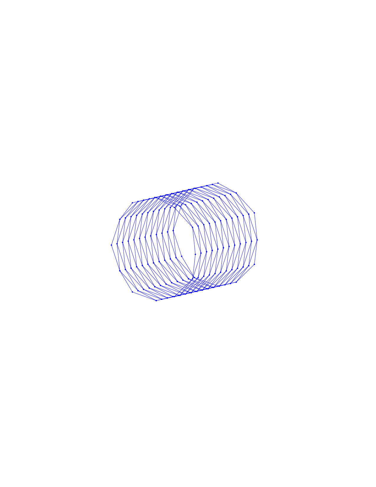 Figure 1
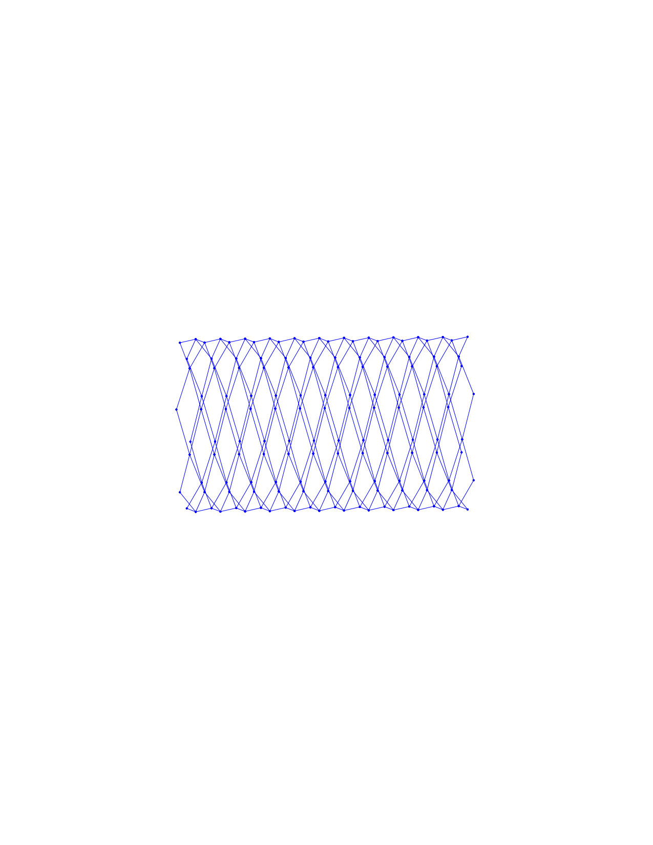 Figure 2
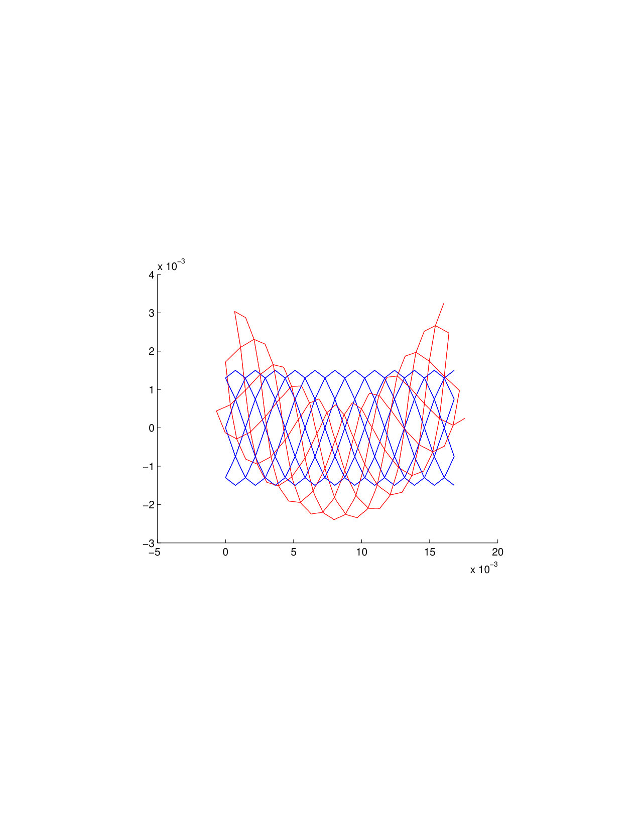 Figure 3
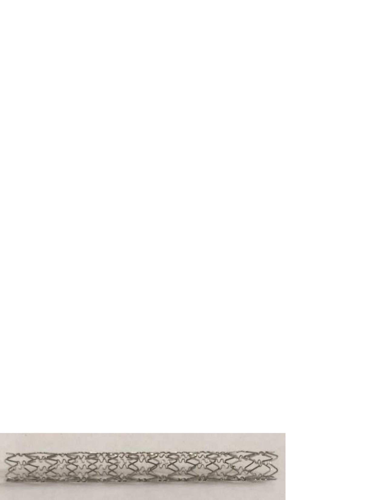 Figure 4
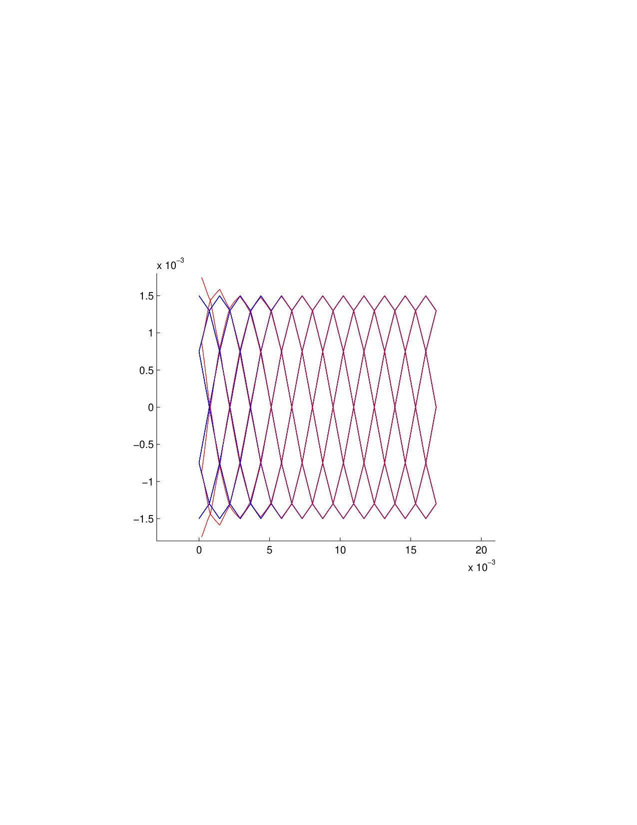 Figure 5
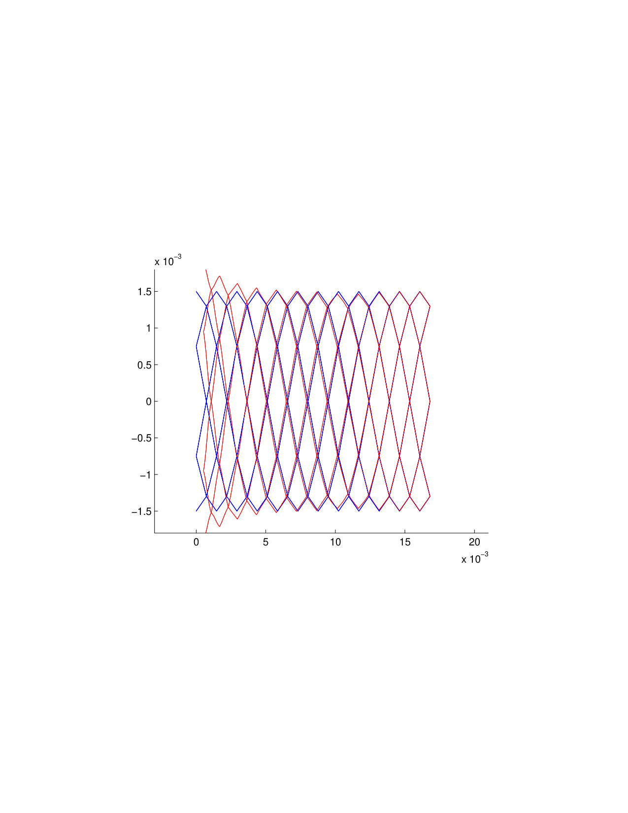 Figure 6
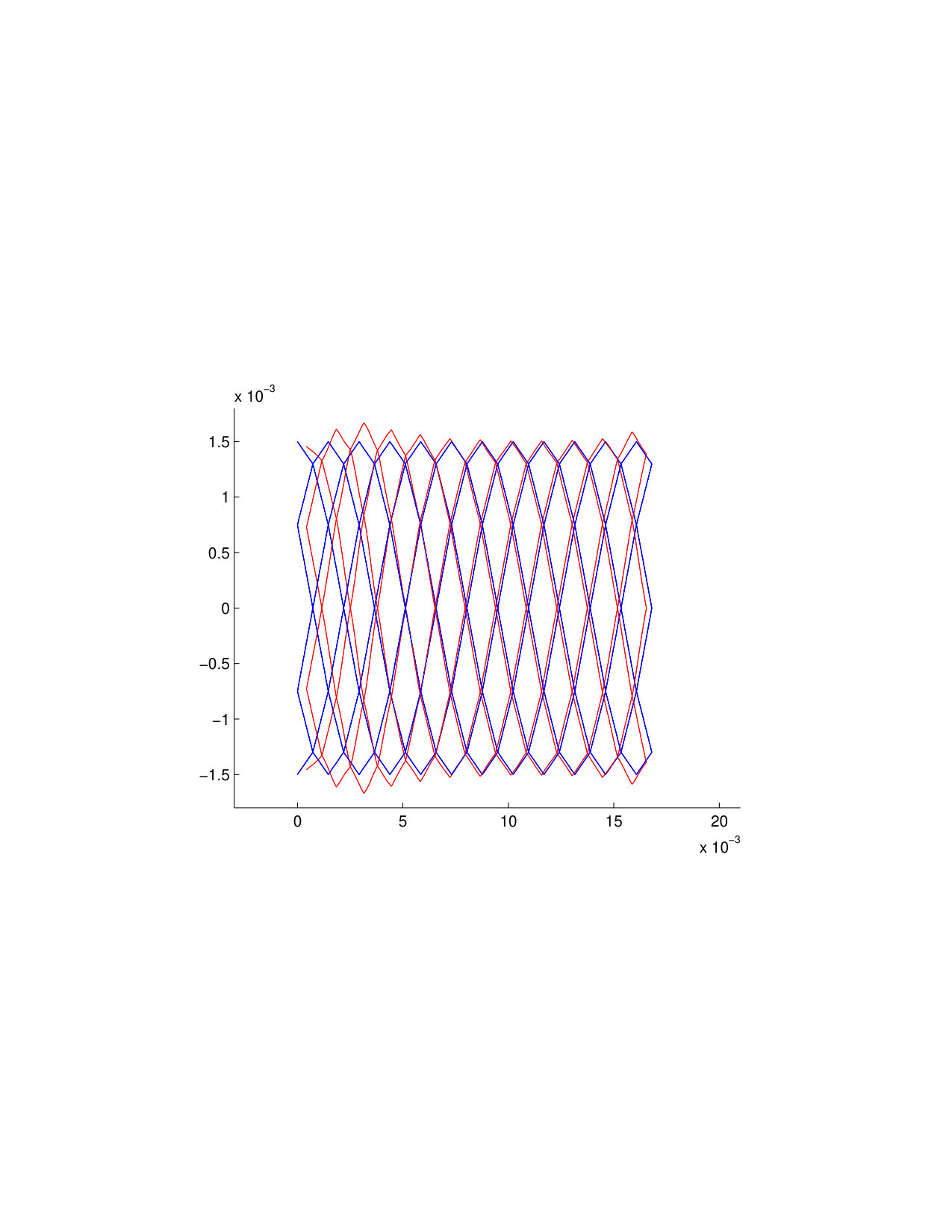 Figure 7
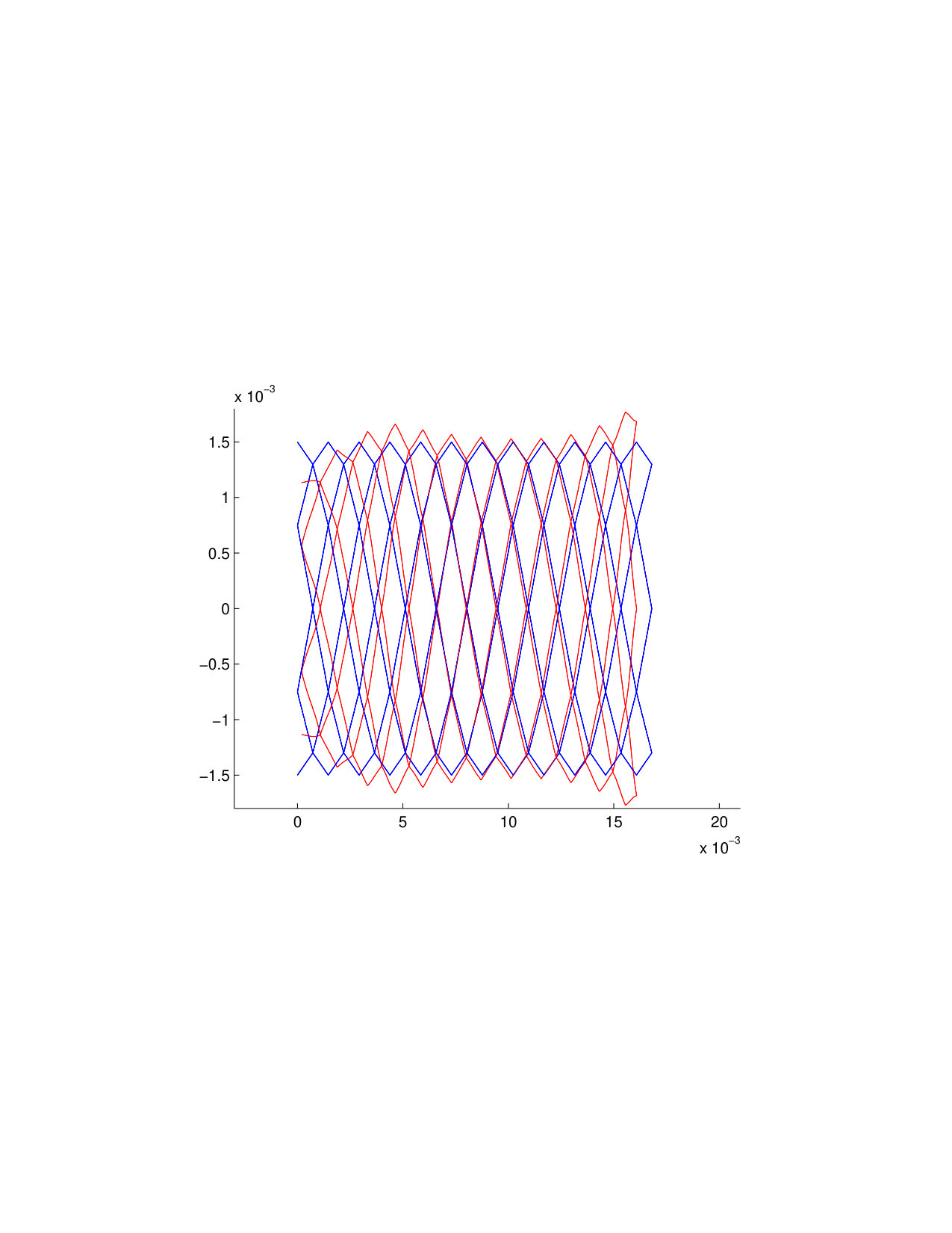 Figure 8
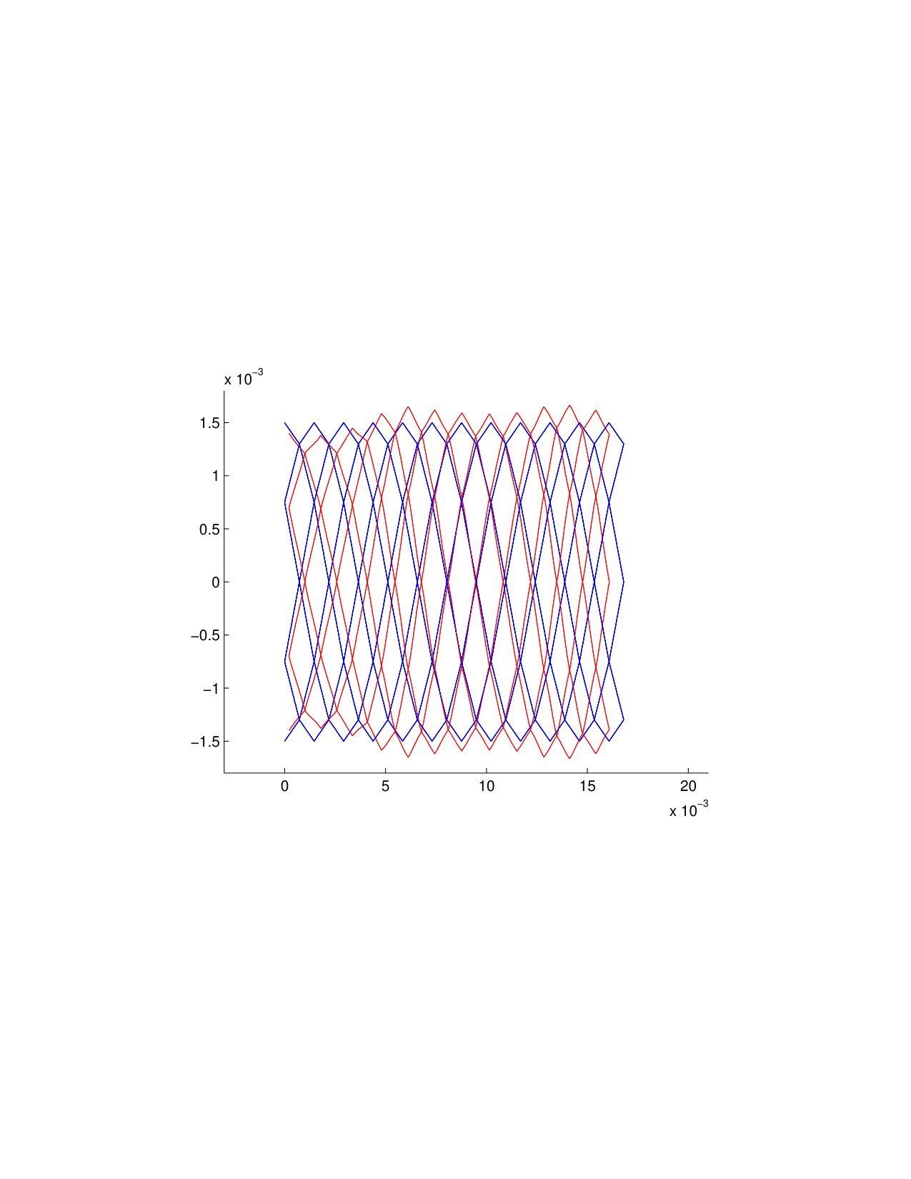 Figure 9
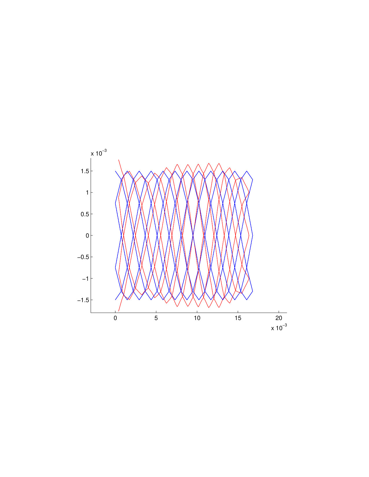 Figure 10
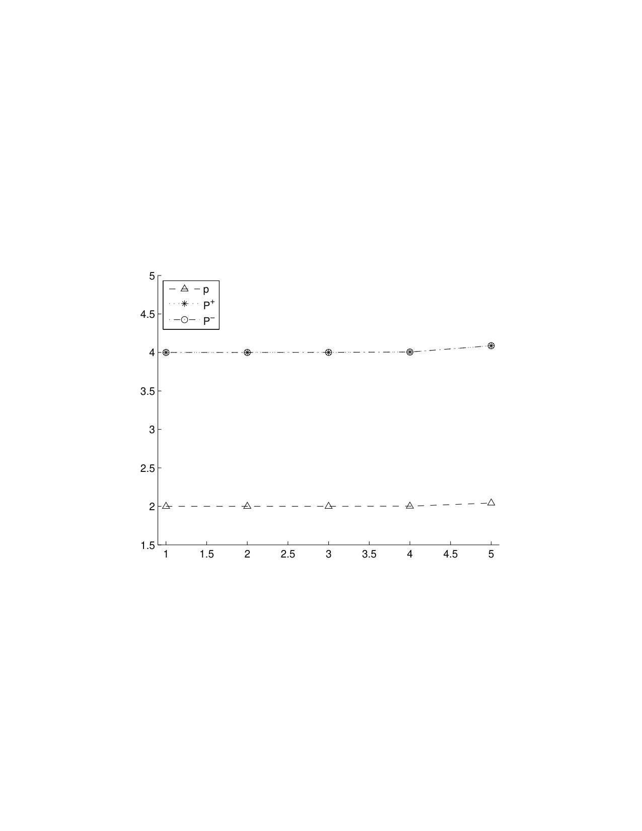 Figure 11
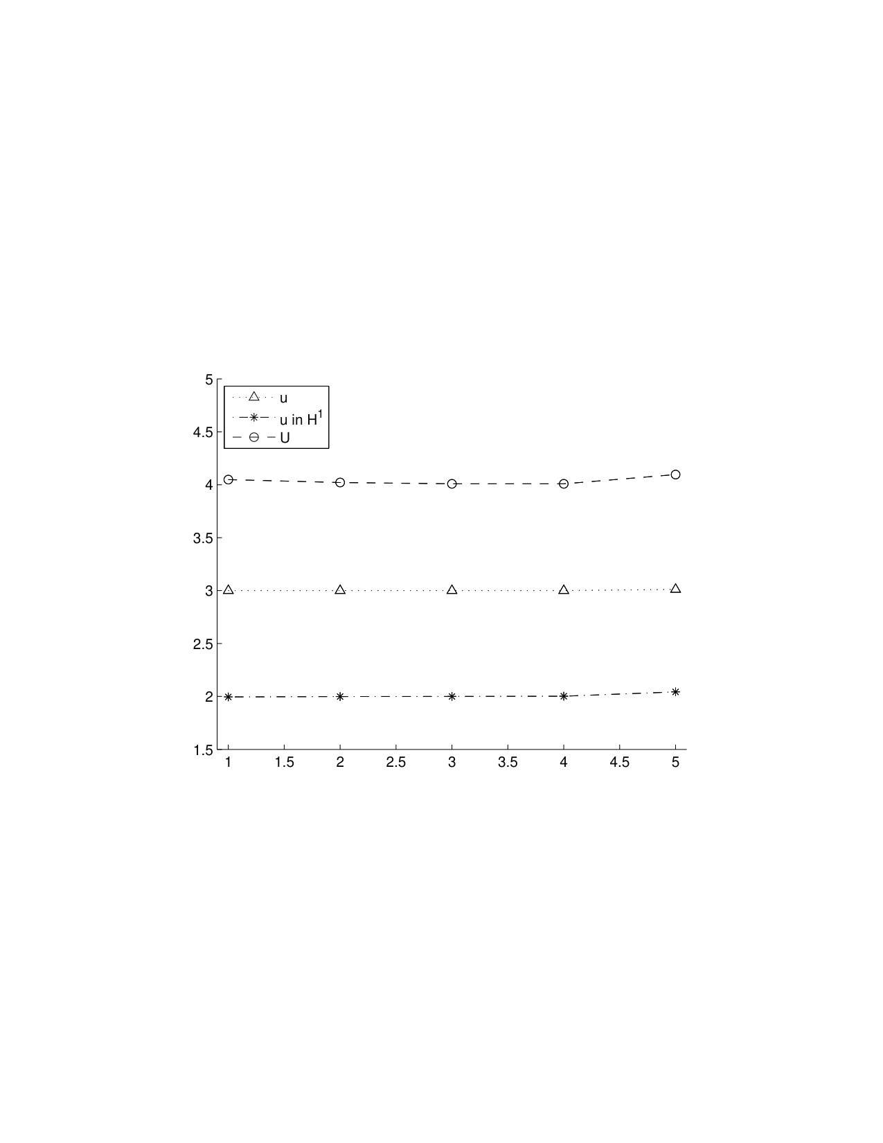 Figure 12
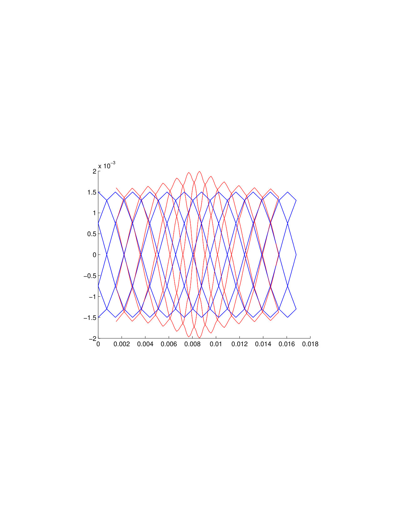 Figure 13
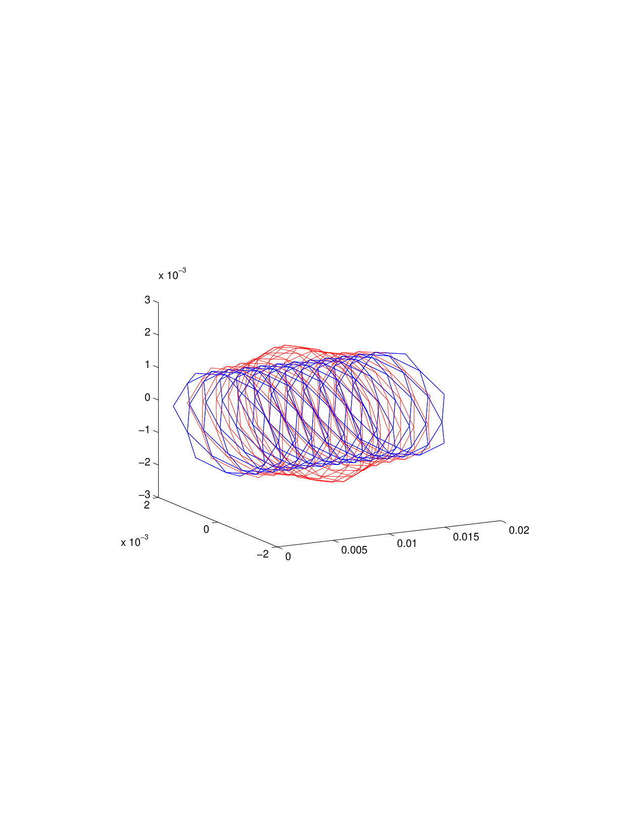 Figure 14
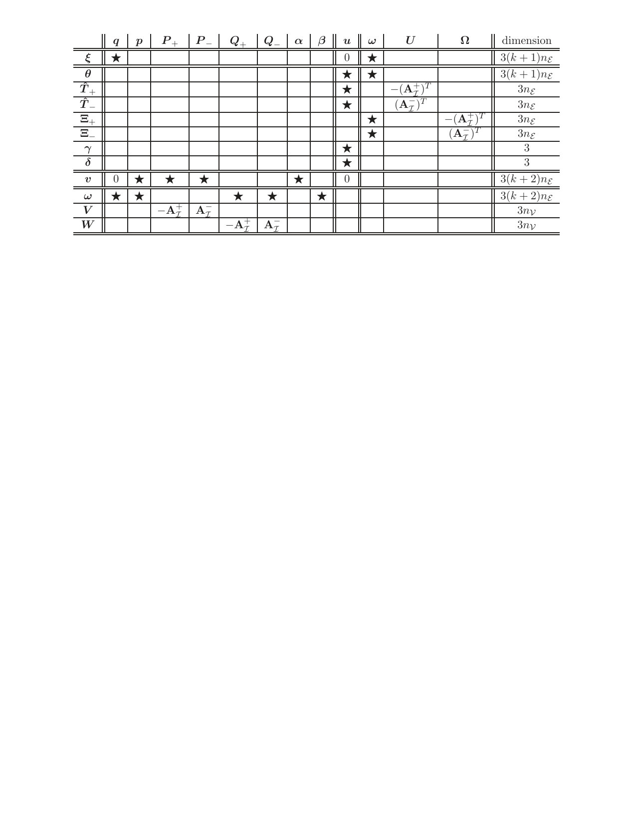 Figure 15
| splitting | |||||
|---|---|---|---|---|---|
| 2 | 1.8127e-5 | 3.1945266e-8 | 3.2871209e-8 | 8.52118e-4 | 3.3700235e-5 |
| 4 | 0.4532e-5 | 0.1995776e-8 | 0.2024711e-8 | 1.06516e-4 | 0.2116646e-5 |
| 8 | 0.1133e-5 | 0.0124898e-8 | 0.0125802e-8 | 0.13314e-4 | 0.0132275e-5 |
| 16 | 0.0283e-5 | 0.0007811e-8 | 0.0007839e-8 | 0.01664e-4 | 0.0008260e-5 |
| 32 | 0.0070e-5 | 0.0000486e-8 | 0.0000487e-8 | 0.00208e-4 | 0.0000514e-5 |
| 64 | 0.0017e-5 | 0.0000028e-8 | 0.0000028e-8 | 0.00025e-4 | 0.0000030e-5 |
| new formulation | old formulation | |||
|---|---|---|---|---|
| splitting | comp. time in | size of matrix | comp. time in | size of matrix |
| 8 | 22 | 105198 | 2 | 38958 |
| 16 | 47 | 211182 | 42 | 78702 |
| 32 | 108 | 423150 | 152 | 158190 |
| 64 | 288 | 847086 | 629 | 317166 |
| 128 | 903 | 1694958 | 4183 | 635118 |
| no LDL | using LDLT | |||
|---|---|---|---|---|
| splits | size of matrix | time (s) | time for precomputation (s) | time for iterations (s) |
| 12462 | 476 | 1.34 | 110 | |
| 25710 | 554 | 1.70 | 203 | |
| 52206 | 793 | 4.62 | 392 | |
| 105198 | 1338 | 23.71 | 855 | |
| no LDL | using LDLT | ||
|---|---|---|---|
| time (s) | time for precomputation (s) | time for iterations (s) | |
| 277 | 3.66 | 202 | |
| 554 | 1.77 | 392 | |
| 1120 | 1.52 | 808 | |
| 2332 | 1.39 | 1717 | |
| error | |
|---|---|
| error | |
|---|---|
Peer Reviews
No public reviews on file for this paper yet. If you reviewed it on a platform where reviews are public (OpenReview, ICLR, NeurIPS, ICML), you can paste yours below so the community can read it here.
Videos
No videos yet. Explain this paper in a talk, walkthrough, or lecture? Add one.
Taxonomy
TopicsElasticity and Material Modeling · Dynamics and Control of Mechanical Systems · Advanced Numerical Methods in Computational Mathematics
Modeling and discretization methods for the
numerical simulation of elastic stents ††thanks: Received… Accepted… Published online on… Recommended by…. This work has been supported by Deutscher Akademischer Austauschdienst (DAAD) via Project Asymptotic and algebraic analysis of nonlinear eigenvalue problems in contact mechanics and electro magnetism. The third author is also supported by Einstein Foundation Berlin via Einstein Center ECMath Project: Model Reduction for Nonlinear Parameter-Dependent Eigenvalue Problems in Photonic Crystals.
Luka Grubišić222Department of Mathematics, Faculty of Science, University of Zagreb, Bijenička 30, 10000 Zagreb, {luka,mljulj,tambaca}@math.hr.
Matko Ljulj222Department of Mathematics, Faculty of Science, University of Zagreb, Bijenička 30, 10000 Zagreb, {luka,mljulj,tambaca}@math.hr.
Volker Mehrmann33footnotemark: 3
Josip Tambača222Department of Mathematics, Faculty of Science, University of Zagreb, Bijenička 30, 10000 Zagreb, {luka,mljulj,tambaca}@math.hr.
Abstract
A new model description for the numerical simulation of elastic stents is proposed. Based on the new formulation an - inequality for the finite element discretization is proved and the proof of the - inequality for the continuous problem is simplified. The new formulation also leads to faster simulation times despite an increased number of variables. The techniques also simplify the analysis and numerical solution of the evolution problem describing the movement of the stent under external forces. The results are illustrated via numerical examples.
44footnotetext: Institut für Mathematik MA 4-5, TU Berlin, Str. des 17. Juni 136, D-10623 Berlin, FRG. [email protected].
Keywords: elastic stent, mathematical modeling, numerical simulation, mixed finite element formulation, stationary system, evolution equation,
Ams Subj. Classification: 74S05, 74K10, 74K30, 74G15, 74H15, 65M15, 65M60
1 Introduction
In this paper we present a new model description for the dynamic and stationary simulation of stents. This new formulation is using constrained partial differential equations in mixed variational weak form, which are based on a network structure consisting of one dimensional curved rods (struts). The new formulation will turn out to be particularly convenient for the analysis of the partial differential equation, in particular in proving an - inequality which directly transfers to a discrete - inequality in the discretized setting, so that from classical results of [3] the error estimates follow.
In the new formulation, the inextensibility and unshearability of the rod are expressed in the weak formulation, but the continuity of the displacement and the modeling of infinitesimal rotations are modelled via constraints so that they do not have to be incorporated in the function spaces as was done in the classical approach in [10]. This advantage of the new formulation comes along with the introduction of new unknowns for the displacements and infinitesimal rotations at vertices where different struts are connected and further unknowns for the contact couples and contact forces at the end points of each strut. However, despite the introduction of many new unknowns, the numerical solvers become more efficient for the large scale cases.
Stents, see Figure 1, are typically considered as a union of struts each of which is modeled by a 1D curved rod model, see [14, 15], and a set of junction conditions describing the connection of the struts, see [9]. The so-obtained model describes the three-dimensional behavior of stents but it has the complexity of a one-dimensional model. This model can be applied for any elastic structure made of thin curved (or straight) rods. It was first formulated in [23] and then reformulated in the weak form in [5]. The properties of the mixed formulation for the model have been analyzed in [10], numerical methods have been introduced, and error estimates have been derived in [12], but up to now error estimates for the contact forces, which are represented as Lagrange multipliers of the contact conditions, were missing. To derive these error estimates is one of the main results of this paper.
To model the topology of the stent we use an undirected graph consisting of a set of vertices, which are the points where the middle lines of the rods meet and a set of edges that represent a 1D description of the curved rod. To be able to use a 1D curved rod model, we additionally need to prescribe the local geometry of the rod, i.e., the middle curve and the geometry of the cross-section as well as the material properties of the stent. These are given by
- •
the function {\mathchoice{\mbox{\boldmath\displaystyle\Phi}}{\mbox{\boldmath\textstyle\Phi}}{\mbox{\boldmath\scriptstyle\Phi}}{\mbox{\boldmath\scriptscriptstyle\Phi}}}^{i}:[0,\ell^{i}]\to{\mathbb{R}}^{3} as natural parametrization of the middle line of the th strut of length , represented by the edge {\mathchoice{\mbox{\boldmath\displaystyle e}}{\mbox{\boldmath\textstyle e}}{\mbox{\boldmath\scriptstyle e}}{\mbox{\boldmath\scriptscriptstyle e}}}^{i}\in{\cal E},
- •
the shear modulus and the Young modulus as parameters describing the material of the th strut,
- •
as well as the width and the thickness of the rectangular cross-section of the th strut.
Using these quantities, in the stationary case, see [23], the model for the th strut , is given by the following system of ordinary differential equations (in space)
[TABLE]
where for the th strut
- •
{\mathchoice{\mbox{\boldmath\displaystyle u}}{\mbox{\boldmath\textstyle u}}{\mbox{\boldmath\scriptstyle u}}{\mbox{\boldmath\scriptscriptstyle u}}}^{i}:[0,\ell^{i}]\to{\mathbb{R}}^{3} denotes the vector of displacements on the middle curve,
- •
{\mathchoice{\mbox{\boldmath\displaystyle\omega}}{\mbox{\boldmath\textstyle\omega}}{\mbox{\boldmath\scriptstyle\omega}}{\mbox{\boldmath\scriptscriptstyle\omega}}}^{i}:[0,\ell^{i}]\to{\mathbb{R}}^{3} is the vector of infinitesimal rotations of the cross-section,
- •
{\mathchoice{\mbox{\boldmath\displaystyle q}}{\mbox{\boldmath\textstyle q}}{\mbox{\boldmath\scriptstyle q}}{\mbox{\boldmath\scriptscriptstyle q}}}^{i} is the contact moment and {\mathchoice{\mbox{\boldmath\displaystyle p}}{\mbox{\boldmath\textstyle p}}{\mbox{\boldmath\scriptstyle p}}{\mbox{\boldmath\scriptscriptstyle p}}}^{i} is the contact force,
- •
{\mathchoice{\mbox{\boldmath\displaystyle f}}{\mbox{\boldmath\textstyle f}}{\mbox{\boldmath\scriptstyle f}}{\mbox{\boldmath\scriptscriptstyle f}}}^{i} is the line density of the applied forces,
- •
{\bf Q}^{i}=[{\mathchoice{\mbox{\boldmath\displaystyle t}}{\mbox{\boldmath\textstyle t}}{\mbox{\boldmath\scriptstyle t}}{\mbox{\boldmath\scriptscriptstyle t}}}^{i},{\mathchoice{\mbox{\boldmath\displaystyle n}}{\mbox{\boldmath\textstyle n}}{\mbox{\boldmath\scriptstyle n}}{\mbox{\boldmath\scriptscriptstyle n}}}^{i},{\hbox{\bf b}}^{i}] is an orthogonal rotation matrix associated to the middle curve, with {\mathchoice{\mbox{\boldmath\displaystyle t}}{\mbox{\boldmath\textstyle t}}{\mbox{\boldmath\scriptstyle t}}{\mbox{\boldmath\scriptscriptstyle t}}}^{i}=({\mathchoice{\mbox{\boldmath\displaystyle\Phi}}{\mbox{\boldmath\textstyle\Phi}}{\mbox{\boldmath\scriptstyle\Phi}}{\mbox{\boldmath\scriptscriptstyle\Phi}}}^{i})^{\prime} being the unit tangent to the middle curve and {\mathchoice{\mbox{\boldmath\displaystyle n}}{\mbox{\boldmath\textstyle n}}{\mbox{\boldmath\scriptstyle n}}{\mbox{\boldmath\scriptscriptstyle n}}}^{i}, being vectors spanning the normal plane to the middle curve, so that represents the local basis at each point of the middle curve,
- •
is a positive definite diagonal matrix, with the Young modulus , the shear modulus , , are the moments of inertia of the cross section and is the torsional rigidity of the cross section.
Equations (1.1) and (1.2) represent equilibrium equations (for forces and moments), while (1.3) and (1.4) are constitutive relations. In particular, (1.4) describes the inextensibility and unshearability of the struts, see [5] for more details.
In addition to equations (1.1)–(1.4), at each vertex of the stent we have a kinematic coupling condition that and are continuous and a dynamic coupling condition describing the balance of contact forces and contact moments .
Denoting by the set of all edges that leave the th vertex, i.e., the local variable is equal to [math] at vertex and by the set of all edges that enter the vertex, i.e., the local variable is equal to for th edge at the vertex . With these notations we obtain the node conditions
[TABLE]
Since this is a pure traction problem, we can integrate over and specify a unique solution by requiring the two additional conditions
[TABLE]
which means that the total displacement as well as the total infinitesimal rotation are zero.
In the formulation of [10], the model is described on the collection of all displacements {\mathchoice{\mbox{\boldmath\displaystyle u}}{\mbox{\boldmath\textstyle u}}{\mbox{\boldmath\scriptstyle u}}{\mbox{\boldmath\scriptscriptstyle u}}}^{i} and infinitesimal rotations {\mathchoice{\mbox{\boldmath\displaystyle\omega}}{\mbox{\boldmath\textstyle\omega}}{\mbox{\boldmath\scriptstyle\omega}}{\mbox{\boldmath\scriptscriptstyle\omega}}}^{i} for all edges which are continuous on the whole stent. Thus, the tuples of unknowns in the problem {\mathchoice{\mbox{\boldmath\displaystyle u}}{\mbox{\boldmath\textstyle u}}{\mbox{\boldmath\scriptstyle u}}{\mbox{\boldmath\scriptscriptstyle u}}}_{S}=(({\mathchoice{\mbox{\boldmath\displaystyle u}}{\mbox{\boldmath\textstyle u}}{\mbox{\boldmath\scriptstyle u}}{\mbox{\boldmath\scriptscriptstyle u}}}^{1},{\mathchoice{\mbox{\boldmath\displaystyle\omega}}{\mbox{\boldmath\textstyle\omega}}{\mbox{\boldmath\scriptstyle\omega}}{\mbox{\boldmath\scriptscriptstyle\omega}}}^{1}),\ldots,({\mathchoice{\mbox{\boldmath\displaystyle u}}{\mbox{\boldmath\textstyle u}}{\mbox{\boldmath\scriptstyle u}}{\mbox{\boldmath\scriptscriptstyle u}}}^{n_{\cal E}},{\mathchoice{\mbox{\boldmath\displaystyle\omega}}{\mbox{\boldmath\textstyle\omega}}{\mbox{\boldmath\scriptstyle\omega}}{\mbox{\boldmath\scriptscriptstyle\omega}}}^{n_{\cal E}})) belong to the space
[TABLE]
with being the Sobolov space of functions on whose derivatives up to the first derivative are square Lebesgue integrable. The formulation given in [10] is a mixed formulation with Lagrange multipliers appearing in the formulation due to the inextensibility and unshearability of the struts in the 1d curved rod model (1.4), and the two conditions on the total displacement and infinitesimal rotation (1.6). Under these conditions, in [10] an - inequality was proved and the well-posedness of the problem was established. However, for the discretized problem via the finite element method it would be necessary to also have a discrete - inequality to obtain an error estimate also for the Lagrange multipliers approximation.
We will show that the elastic energy is coercive in the space implementing inextensibility, unshearability, and continuity of displacement and infinitesimal rotation. Using the results of [3], we will show that the Lagrange multipliers are unique in both the old and the new formulation and for the discrete problem also in the new formulation. This is a considerable improvement compared to the classical mixed formulation [12], where a proof of the discrete - inequality was not successful.
Let denote the incidence matrix of the oriented graph with three connected components, organized in the following way: a submatrix at rows and columns is if the edge enters the vertex , if it leaves the vertex or [math] otherwise. Then the matrix is obtained from by setting all elements to [math] and is defined as . Let us also introduce the projectors
[TABLE]
on the coordinates and , respectively. We will also need the spaces
[TABLE]
with associated norms
[TABLE]
The norm corresponding to the last term for is also used as the norm for . For a function {\mathchoice{\mbox{\boldmath\displaystyle y}}{\mbox{\boldmath\textstyle y}}{\mbox{\boldmath\scriptstyle y}}{\mbox{\boldmath\scriptscriptstyle y}}}=({\mathchoice{\mbox{\boldmath\displaystyle y}}{\mbox{\boldmath\textstyle y}}{\mbox{\boldmath\scriptstyle y}}{\mbox{\boldmath\scriptscriptstyle y}}}^{1},\ldots,{\mathchoice{\mbox{\boldmath\displaystyle y}}{\mbox{\boldmath\textstyle y}}{\mbox{\boldmath\scriptstyle y}}{\mbox{\boldmath\scriptscriptstyle y}}}^{n_{\cal E}})\in L^{2}_{H^{1}}({\cal N};{\mathbb{R}}^{3}) by {\mathchoice{\mbox{\boldmath\displaystyle y}}{\mbox{\boldmath\textstyle y}}{\mbox{\boldmath\scriptstyle y}}{\mbox{\boldmath\scriptscriptstyle y}}}^{\prime} we denote (\partial_{s}{\mathchoice{\mbox{\boldmath\displaystyle y}}{\mbox{\boldmath\textstyle y}}{\mbox{\boldmath\scriptstyle y}}{\mbox{\boldmath\scriptscriptstyle y}}}^{1},\ldots,\partial_{s}{\mathchoice{\mbox{\boldmath\displaystyle y}}{\mbox{\boldmath\textstyle y}}{\mbox{\boldmath\scriptstyle y}}{\mbox{\boldmath\scriptscriptstyle y}}}^{n_{\cal E}})\in L^{2}({\cal N};{\mathbb{R}}^{3}).
The results that we prove for the continuous model in Section 3 hold for general geometries, while the results for the discrete approximation in Section 4 are proved only for stent geometries with straight struts.
The paper is organized as follows. In Section 2 we present the new formulation of the stent model. In Section 3 we analyze the new model and give a proof of the inf-sup inequality for the weak formulation of the continuous infinite dimensional model and in Section 4 we analyze the discrete model that is obtained after finite element discretization and show a corresponding inf-sup inequality. Finally in Section 5 we study the dynamical system of the stent movement under excitation forces. We analyze the properties and present numerical simulation results.
2 New formulation of the model
In this section we reformulate the stent model in a way that enables the proof of a discrete - inequality and then, using classical results, appropriate error estimates follow. For this, we treat all unknowns in the problem explicitly and do not encode them in the function spaces or the weak formulation. In this way not only the inextensibility and unshearability of the rod is expressed in the weak formulation, but the continuity of the displacement and infinitesimal rotation is reflected in the function space of the mixed formulation in . This leads to the introduction of new unknowns, displacements and infinitesimal rotations at vertices, and further, the contact moments and contact forces at the ends of each strut.
Since and are continuous over the whole stent, we introduce as extra variables the displacements and infinitesimal rotations at the vertices {\mathchoice{\mbox{\boldmath\displaystyle U}}{\mbox{\boldmath\textstyle U}}{\mbox{\boldmath\scriptstyle U}}{\mbox{\boldmath\scriptscriptstyle U}}}^{i},{\mathchoice{\mbox{\boldmath\displaystyle\Omega}}{\mbox{\boldmath\textstyle\Omega}}{\mbox{\boldmath\scriptstyle\Omega}}{\mbox{\boldmath\scriptscriptstyle\Omega}}}^{i}, , and then form the vectors
[TABLE]
Then the kinematic coupling at the vertex leads to the conditions
[TABLE]
To express the dynamic coupling conditions, we introduce the contact moments and forces at the ends of the struts,
[TABLE]
and define
[TABLE]
Then the dynamic coupling conditions at the vertex can be expressed as
[TABLE]
Equations (1.1)–(1.4), (2.1), (2.2), (2.3), and (1.6) together constitute the stent problem in our new formulation for which we now derive in detail the weak formulation.
We multiply the th equation of (1.1) by {\mathchoice{\mbox{\boldmath\displaystyle v}}{\mbox{\boldmath\textstyle v}}{\mbox{\boldmath\scriptstyle v}}{\mbox{\boldmath\scriptscriptstyle v}}}^{i}\in H^{1}(0,\ell^{i};{\mathbb{R}}^{3}) and that of (1.2) by {\mathchoice{\mbox{\boldmath\displaystyle w}}{\mbox{\boldmath\textstyle w}}{\mbox{\boldmath\scriptstyle w}}{\mbox{\boldmath\scriptscriptstyle w}}}^{i}\in H^{1}(0,\ell^{i};{\mathbb{R}}^{3}), add them, integrate over , and sum the equations over . This yields
[TABLE]
After partial integration we obtain
[TABLE]
i.e.,
[TABLE]
In a similar way we multiply (1.3) by {\mathchoice{\mbox{\boldmath\displaystyle\xi}}{\mbox{\boldmath\textstyle\xi}}{\mbox{\boldmath\scriptstyle\xi}}{\mbox{\boldmath\scriptscriptstyle\xi}}}^{i}\in L^{2}(0,\ell^{i};{\mathbb{R}}^{3}) and (1.4) by integrate over and sum all equations to obtain
[TABLE]
We also multiply the equations in (2.3) for the th vertex by {\mathchoice{\mbox{\boldmath\displaystyle V}}{\mbox{\boldmath\textstyle V}}{\mbox{\boldmath\scriptstyle V}}{\mbox{\boldmath\scriptscriptstyle V}}}^{j} and {\mathchoice{\mbox{\boldmath\displaystyle W}}{\mbox{\boldmath\textstyle W}}{\mbox{\boldmath\scriptstyle W}}{\mbox{\boldmath\scriptscriptstyle W}}}^{j} from , respectively, and sum the equations over which gives
[TABLE]
Since \sum_{i\in J^{+}_{j}}{\mathchoice{\mbox{\boldmath\displaystyle P}}{\mbox{\boldmath\textstyle P}}{\mbox{\boldmath\scriptstyle P}}{\mbox{\boldmath\scriptscriptstyle P}}}^{i}_{+}=\mathbb{P}^{j}_{\cal V}{\bf A}^{+}_{\cal I}{\mathchoice{\mbox{\boldmath\displaystyle P}}{\mbox{\boldmath\textstyle P}}{\mbox{\boldmath\scriptstyle P}}{\mbox{\boldmath\scriptscriptstyle P}}}_{+} and \sum_{i\in J^{-}_{j}}{\mathchoice{\mbox{\boldmath\displaystyle P}}{\mbox{\boldmath\textstyle P}}{\mbox{\boldmath\scriptstyle P}}{\mbox{\boldmath\scriptscriptstyle P}}}^{i}_{-}=\mathbb{P}^{j}_{\cal V}{\bf A}^{-}_{\cal I}{\mathchoice{\mbox{\boldmath\displaystyle P}}{\mbox{\boldmath\textstyle P}}{\mbox{\boldmath\scriptstyle P}}{\mbox{\boldmath\scriptscriptstyle P}}}_{-}, this equation can be written as
[TABLE]
and, therefore,
[TABLE]
for all {\mathchoice{\mbox{\boldmath\displaystyle V}}{\mbox{\boldmath\textstyle V}}{\mbox{\boldmath\scriptstyle V}}{\mbox{\boldmath\scriptscriptstyle V}}}=[{\mathchoice{\mbox{\boldmath\displaystyle V}}{\mbox{\boldmath\textstyle V}}{\mbox{\boldmath\scriptstyle V}}{\mbox{\boldmath\scriptscriptstyle V}}}^{1},\ldots,{\mathchoice{\mbox{\boldmath\displaystyle V}}{\mbox{\boldmath\textstyle V}}{\mbox{\boldmath\scriptstyle V}}{\mbox{\boldmath\scriptscriptstyle V}}}^{n_{\cal V}}]^{T}, {\mathchoice{\mbox{\boldmath\displaystyle W}}{\mbox{\boldmath\textstyle W}}{\mbox{\boldmath\scriptstyle W}}{\mbox{\boldmath\scriptscriptstyle W}}}=[{\mathchoice{\mbox{\boldmath\displaystyle W}}{\mbox{\boldmath\textstyle W}}{\mbox{\boldmath\scriptstyle W}}{\mbox{\boldmath\scriptscriptstyle W}}}^{1},\ldots,{\mathchoice{\mbox{\boldmath\displaystyle W}}{\mbox{\boldmath\textstyle W}}{\mbox{\boldmath\scriptstyle W}}{\mbox{\boldmath\scriptscriptstyle W}}}^{n_{\cal V}}]^{T}\in{\mathbb{R}}^{3n_{\cal V}}.
Multiplying the equations for the displacements in (2.1) by {\mathchoice{\mbox{\boldmath\displaystyle\Theta}}{\mbox{\boldmath\textstyle\Theta}}{\mbox{\boldmath\scriptstyle\Theta}}{\mbox{\boldmath\scriptscriptstyle\Theta}}}^{i}_{+} and {\mathchoice{\mbox{\boldmath\displaystyle\Theta}}{\mbox{\boldmath\textstyle\Theta}}{\mbox{\boldmath\scriptstyle\Theta}}{\mbox{\boldmath\scriptscriptstyle\Theta}}}^{i}_{-}, we obtain
[TABLE]
Since \mathbb{P}^{i}_{\cal E}({\bf A}^{+}_{\cal I})^{T}{\mathchoice{\mbox{\boldmath\displaystyle U}}{\mbox{\boldmath\textstyle U}}{\mbox{\boldmath\scriptstyle U}}{\mbox{\boldmath\scriptscriptstyle U}}}={\mathchoice{\mbox{\boldmath\displaystyle U}}{\mbox{\boldmath\textstyle U}}{\mbox{\boldmath\scriptstyle U}}{\mbox{\boldmath\scriptscriptstyle U}}}^{j} for , for {\mathchoice{\mbox{\boldmath\displaystyle\Theta}}{\mbox{\boldmath\textstyle\Theta}}{\mbox{\boldmath\scriptstyle\Theta}}{\mbox{\boldmath\scriptscriptstyle\Theta}}}_{\pm}=[{\mathchoice{\mbox{\boldmath\displaystyle\Theta}}{\mbox{\boldmath\textstyle\Theta}}{\mbox{\boldmath\scriptstyle\Theta}}{\mbox{\boldmath\scriptscriptstyle\Theta}}}^{1}_{\pm},\ldots,{\mathchoice{\mbox{\boldmath\displaystyle\Theta}}{\mbox{\boldmath\textstyle\Theta}}{\mbox{\boldmath\scriptstyle\Theta}}{\mbox{\boldmath\scriptscriptstyle\Theta}}}^{n_{\cal E}}_{\pm}]^{T} we have
[TABLE]
and similarly, for the rotations, using the notation {\mathchoice{\mbox{\boldmath\displaystyle\Xi}}{\mbox{\boldmath\textstyle\Xi}}{\mbox{\boldmath\scriptstyle\Xi}}{\mbox{\boldmath\scriptscriptstyle\Xi}}}_{\pm}=[{\mathchoice{\mbox{\boldmath\displaystyle\Xi}}{\mbox{\boldmath\textstyle\Xi}}{\mbox{\boldmath\scriptstyle\Xi}}{\mbox{\boldmath\scriptscriptstyle\Xi}}}^{1}_{\pm},\ldots,{\mathchoice{\mbox{\boldmath\displaystyle\Xi}}{\mbox{\boldmath\textstyle\Xi}}{\mbox{\boldmath\scriptstyle\Xi}}{\mbox{\boldmath\scriptscriptstyle\Xi}}}^{n_{\cal E}}_{\pm}]^{T}, we get
[TABLE]
Thus, we have
[TABLE]
for the displacements and
[TABLE]
for the rotations. We multiply the equations (1.6) by and , respectively, and summing up, we obtain
[TABLE]
Subtracting (2.6) from (2.4), we obtain
[TABLE]
We then add (2.7) and (2.8) to (2.5) and obtain
[TABLE]
In [10] and [12] the mixed formulation of the stent model was presented using the space for the displacement vector and the infinitesimal rotation vector . The space for the Lagrange multipliers {\mathchoice{\mbox{\boldmath\displaystyle p}}{\mbox{\boldmath\textstyle p}}{\mbox{\boldmath\scriptstyle p}}{\mbox{\boldmath\scriptscriptstyle p}}},{\mathchoice{\mbox{\boldmath\displaystyle\alpha}}{\mbox{\boldmath\textstyle\alpha}}{\mbox{\boldmath\scriptstyle\alpha}}{\mbox{\boldmath\scriptscriptstyle\alpha}}},{\mathchoice{\mbox{\boldmath\displaystyle\beta}}{\mbox{\boldmath\textstyle\beta}}{\mbox{\boldmath\scriptstyle\beta}}{\mbox{\boldmath\scriptscriptstyle\beta}}}, and the continuity conditions for displacements and infinitesimal rotations were inherently built into the space . We now relax these conditions and consider them as additional equations in the problem and enlarge the space of unknowns by adding further Lagrange multipliers. The resulting function spaces are given by
[TABLE]
To simplify the notation for the elements of these spaces we introduce
[TABLE]
for the unknowns in the problem and
[TABLE]
for the associated test functions.
In this notation, the bilinear forms and the linear functionals that appear in the above calculations are given by
[TABLE]
Then the variational formulation (2.10), (2.11) and (2.9) can be expressed as follows.
Determine {\mathchoice{\mbox{\boldmath\displaystyle\Sigma}}{\mbox{\boldmath\textstyle\Sigma}}{\mbox{\boldmath\scriptstyle\Sigma}}{\mbox{\boldmath\scriptscriptstyle\Sigma}}}\in V and {\mathchoice{\mbox{\boldmath\displaystyle\phi}}{\mbox{\boldmath\textstyle\phi}}{\mbox{\boldmath\scriptstyle\phi}}{\mbox{\boldmath\scriptscriptstyle\phi}}}\in M such that
[TABLE]
In this way we have obtained that the solution of the stent problem as formulated in (1.1)–(1.6) satisfies (2.12) and conversely that any solution of (2.12) satisfies (1.1)–(1.6).
In this section we have reformulated the mathematical formulation of the stent model by including the continuity conditions at the nodes as extra equations and by adding further Lagrange multipliers. In the next sections, we will use this formulation to obtain a discrete - inequality and to present a simpler proof of the continuous - inequality.
3 Properties of the continuous model
In this section we consider the properties of the continuous operator equation (2.12). For the operator defined by
[TABLE]
we have the adjoint operator (we use the matrix notation to illustrate the similarity to the discrete case discussed later), which satisfies
[TABLE]
Then , the kernel of , is defined as a set of vector functions {\mathchoice{\mbox{\boldmath\displaystyle\psi}}{\mbox{\boldmath\textstyle\psi}}{\mbox{\boldmath\scriptstyle\psi}}{\mbox{\boldmath\scriptscriptstyle\psi}}}=({\mathchoice{\mbox{\boldmath\displaystyle v}}{\mbox{\boldmath\textstyle v}}{\mbox{\boldmath\scriptstyle v}}{\mbox{\boldmath\scriptscriptstyle v}}},{\mathchoice{\mbox{\boldmath\displaystyle w}}{\mbox{\boldmath\textstyle w}}{\mbox{\boldmath\scriptstyle w}}{\mbox{\boldmath\scriptscriptstyle w}}},{\mathchoice{\mbox{\boldmath\displaystyle V}}{\mbox{\boldmath\textstyle V}}{\mbox{\boldmath\scriptstyle V}}{\mbox{\boldmath\scriptscriptstyle V}}},{\mathchoice{\mbox{\boldmath\displaystyle W}}{\mbox{\boldmath\textstyle W}}{\mbox{\boldmath\scriptstyle W}}{\mbox{\boldmath\scriptscriptstyle W}}})\in M such that
[TABLE]
so that {\mathchoice{\mbox{\boldmath\displaystyle\psi}}{\mbox{\boldmath\textstyle\psi}}{\mbox{\boldmath\scriptstyle\psi}}{\mbox{\boldmath\scriptscriptstyle\psi}}}=({\mathchoice{\mbox{\boldmath\displaystyle v}}{\mbox{\boldmath\textstyle v}}{\mbox{\boldmath\scriptstyle v}}{\mbox{\boldmath\scriptscriptstyle v}}},{\mathchoice{\mbox{\boldmath\displaystyle w}}{\mbox{\boldmath\textstyle w}}{\mbox{\boldmath\scriptstyle w}}{\mbox{\boldmath\scriptscriptstyle w}}},{\mathchoice{\mbox{\boldmath\displaystyle V}}{\mbox{\boldmath\textstyle V}}{\mbox{\boldmath\scriptstyle V}}{\mbox{\boldmath\scriptscriptstyle V}}},{\mathchoice{\mbox{\boldmath\displaystyle W}}{\mbox{\boldmath\textstyle W}}{\mbox{\boldmath\scriptstyle W}}{\mbox{\boldmath\scriptscriptstyle W}}})\in\mathop{\rm Ker}\nolimits B^{T} if and only if
[TABLE]
The conditions (3.3) and (3.4) imply that and are continuous on the complete stent, i.e., {\mathchoice{\mbox{\boldmath\displaystyle v}}{\mbox{\boldmath\textstyle v}}{\mbox{\boldmath\scriptstyle v}}{\mbox{\boldmath\scriptscriptstyle v}}},{\mathchoice{\mbox{\boldmath\displaystyle w}}{\mbox{\boldmath\textstyle w}}{\mbox{\boldmath\scriptstyle w}}{\mbox{\boldmath\scriptscriptstyle w}}}\in H^{1}({\cal N};{\mathbb{R}}^{3}). The conditions in (3.1) imply then that is constant on the complete stent and from (3.2) we obtain {\mathchoice{\mbox{\boldmath\displaystyle w}}{\mbox{\boldmath\textstyle w}}{\mbox{\boldmath\scriptstyle w}}{\mbox{\boldmath\scriptscriptstyle w}}}=0. Analogously, from (3.1) we obtain that {\mathchoice{\mbox{\boldmath\displaystyle v}}{\mbox{\boldmath\textstyle v}}{\mbox{\boldmath\scriptstyle v}}{\mbox{\boldmath\scriptscriptstyle v}}}=0, and hence {\mathchoice{\mbox{\boldmath\displaystyle V}}{\mbox{\boldmath\textstyle V}}{\mbox{\boldmath\scriptstyle V}}{\mbox{\boldmath\scriptscriptstyle V}}}={\mathchoice{\mbox{\boldmath\displaystyle W}}{\mbox{\boldmath\textstyle W}}{\mbox{\boldmath\scriptstyle W}}{\mbox{\boldmath\scriptscriptstyle W}}}=0. Thus we have proved the following lemma.
Lemma 1
.
As next step we prove that is closed. For this we derive a kind of Poincaré inequality on the graph , using the notation {\mathchoice{\mbox{\boldmath\displaystyle v}}{\mbox{\boldmath\textstyle v}}{\mbox{\boldmath\scriptstyle v}}{\mbox{\boldmath\scriptscriptstyle v}}}(\ell)=[{\mathchoice{\mbox{\boldmath\displaystyle v}}{\mbox{\boldmath\textstyle v}}{\mbox{\boldmath\scriptstyle v}}{\mbox{\boldmath\scriptscriptstyle v}}}^{1}(\ell^{1}),\ldots,{\mathchoice{\mbox{\boldmath\displaystyle v}}{\mbox{\boldmath\textstyle v}}{\mbox{\boldmath\scriptstyle v}}{\mbox{\boldmath\scriptscriptstyle v}}}^{n_{\cal E}}(\ell^{n_{\cal E}})]^{T}.
Lemma 2
There exists a constant such that for all {\mathchoice{\mbox{\boldmath\displaystyle v}}{\mbox{\boldmath\textstyle v}}{\mbox{\boldmath\scriptstyle v}}{\mbox{\boldmath\scriptscriptstyle v}}}\in L^{2}_{H^{1}}({\cal N};{\mathbb{R}}^{3}) and all {\mathchoice{\mbox{\boldmath\displaystyle V}}{\mbox{\boldmath\textstyle V}}{\mbox{\boldmath\scriptstyle V}}{\mbox{\boldmath\scriptscriptstyle V}}}\in{\mathbb{R}}^{3n_{\cal V}} the following inequality holds
[TABLE]
Proof. Suppose the contrary, i.e., for all constants there exist {\mathchoice{\mbox{\boldmath\displaystyle v}}{\mbox{\boldmath\textstyle v}}{\mbox{\boldmath\scriptstyle v}}{\mbox{\boldmath\scriptscriptstyle v}}}_{C}\in L^{2}_{H^{1}}({\cal N};{\mathbb{R}}^{3}) and {\mathchoice{\mbox{\boldmath\displaystyle V}}{\mbox{\boldmath\textstyle V}}{\mbox{\boldmath\scriptstyle V}}{\mbox{\boldmath\scriptscriptstyle V}}}_{C}\in{\mathbb{R}}^{3n_{\cal V}} such that the opposite inequality holds. Then, for , there exist sequences {\mathchoice{\mbox{\boldmath\displaystyle v}}{\mbox{\boldmath\textstyle v}}{\mbox{\boldmath\scriptstyle v}}{\mbox{\boldmath\scriptscriptstyle v}}}_{k}\in L^{2}_{H^{1}}({\cal N};{\mathbb{R}}^{3}) and {\mathchoice{\mbox{\boldmath\displaystyle V}}{\mbox{\boldmath\textstyle V}}{\mbox{\boldmath\scriptstyle V}}{\mbox{\boldmath\scriptscriptstyle V}}}_{k}\in{\mathbb{R}}^{3n_{\cal V}} such that
[TABLE]
[TABLE]
where, as before, {\mathchoice{\mbox{\boldmath\displaystyle v}}{\mbox{\boldmath\textstyle v}}{\mbox{\boldmath\scriptstyle v}}{\mbox{\boldmath\scriptscriptstyle v}}}_{k}^{\prime} denotes the vector of partial derivatives of {\mathchoice{\mbox{\boldmath\displaystyle v}}{\mbox{\boldmath\textstyle v}}{\mbox{\boldmath\scriptstyle v}}{\mbox{\boldmath\scriptscriptstyle v}}}_{k}. Thus, taking an appropriate subsequence (still indexed by ), we have
[TABLE]
It follows that on each strut we have
[TABLE]
so that {\mathchoice{\mbox{\boldmath\displaystyle v}}{\mbox{\boldmath\textstyle v}}{\mbox{\boldmath\scriptstyle v}}{\mbox{\boldmath\scriptscriptstyle v}}}^{i} is constant on the th strut and
[TABLE]
By the Trace Theorem; see e.g. [7, Section 5.5, Theorem 1] we have then
[TABLE]
Using (3.9) and (3.10), we have
[TABLE]
Since in every block row of size the matrices and have exactly one identity matrix of size we have that {\mathchoice{\mbox{\boldmath\displaystyle V}}{\mbox{\boldmath\textstyle V}}{\mbox{\boldmath\scriptstyle V}}{\mbox{\boldmath\scriptscriptstyle V}}}_{k} is convergent as well. We denote the limit by , and have that its values are given by {\mathchoice{\mbox{\boldmath\displaystyle v}}{\mbox{\boldmath\textstyle v}}{\mbox{\boldmath\scriptstyle v}}{\mbox{\boldmath\scriptscriptstyle v}}}^{i} suitably organized. Therefore, since , subtracting the sequences in (3.11) we obtain that
[TABLE]
Since the rank of is equal to , the kernel of is of dimension by the Rank–Nullity Theorem, [1]. We easily inspect that is spanned by the vectors
[TABLE]
Thus we obtain that all {\mathchoice{\mbox{\boldmath\displaystyle v}}{\mbox{\boldmath\textstyle v}}{\mbox{\boldmath\scriptstyle v}}{\mbox{\boldmath\scriptscriptstyle v}}}^{i} are equal. Since 0=\int_{\cal N}{\mathchoice{\mbox{\boldmath\displaystyle v}}{\mbox{\boldmath\textstyle v}}{\mbox{\boldmath\scriptstyle v}}{\mbox{\boldmath\scriptscriptstyle v}}}=\sum_{i=1}^{n_{\cal E}}\ell^{i}{\mathchoice{\mbox{\boldmath\displaystyle v}}{\mbox{\boldmath\textstyle v}}{\mbox{\boldmath\scriptstyle v}}{\mbox{\boldmath\scriptscriptstyle v}}}^{i}, we obtain that {\mathchoice{\mbox{\boldmath\displaystyle v}}{\mbox{\boldmath\textstyle v}}{\mbox{\boldmath\scriptstyle v}}{\mbox{\boldmath\scriptscriptstyle v}}}^{i}=0 and hence {\mathchoice{\mbox{\boldmath\displaystyle V}}{\mbox{\boldmath\textstyle V}}{\mbox{\boldmath\scriptstyle V}}{\mbox{\boldmath\scriptscriptstyle V}}}=0, which also implies that {\mathchoice{\mbox{\boldmath\displaystyle v}}{\mbox{\boldmath\textstyle v}}{\mbox{\boldmath\scriptstyle v}}{\mbox{\boldmath\scriptscriptstyle v}}}=0. Thus, since
[TABLE]
tends to 0 strongly in for all , which is in contradiction to the unit norm assumption of the sequence, i.e., \|{\mathchoice{\mbox{\boldmath\displaystyle v}}{\mbox{\boldmath\textstyle v}}{\mbox{\boldmath\scriptstyle v}}{\mbox{\boldmath\scriptscriptstyle v}}}_{k}\|_{L^{2}({\cal N};{\mathbb{R}}^{3})}=1.
Proof.
Lemma 3
* is closed.*
Proof. Consider a convergent sequence in , i.e., a sequence of the form
[TABLE]
Then applying the inequality (3.5) to the sequences {\mathchoice{\mbox{\boldmath\displaystyle w}}{\mbox{\boldmath\textstyle w}}{\mbox{\boldmath\scriptstyle w}}{\mbox{\boldmath\scriptscriptstyle w}}}_{k}=({\mathchoice{\mbox{\boldmath\displaystyle w}}{\mbox{\boldmath\textstyle w}}{\mbox{\boldmath\scriptstyle w}}{\mbox{\boldmath\scriptscriptstyle w}}}^{1}_{k},\ldots,{\mathchoice{\mbox{\boldmath\displaystyle w}}{\mbox{\boldmath\textstyle w}}{\mbox{\boldmath\scriptstyle w}}{\mbox{\boldmath\scriptscriptstyle w}}}^{n_{\cal E}}_{k}) and {\mathchoice{\mbox{\boldmath\displaystyle W}}{\mbox{\boldmath\textstyle W}}{\mbox{\boldmath\scriptstyle W}}{\mbox{\boldmath\scriptscriptstyle W}}}_{k}=({\mathchoice{\mbox{\boldmath\displaystyle W}}{\mbox{\boldmath\textstyle W}}{\mbox{\boldmath\scriptstyle W}}{\mbox{\boldmath\scriptscriptstyle W}}}^{1}_{k},\ldots,{\mathchoice{\mbox{\boldmath\displaystyle W}}{\mbox{\boldmath\textstyle W}}{\mbox{\boldmath\scriptstyle W}}{\mbox{\boldmath\scriptscriptstyle W}}}^{n_{\cal E}}_{k}) implies that {\mathchoice{\mbox{\boldmath\displaystyle w}}{\mbox{\boldmath\textstyle w}}{\mbox{\boldmath\scriptstyle w}}{\mbox{\boldmath\scriptscriptstyle w}}}_{k} is bounded in . Therefore, {\mathchoice{\mbox{\boldmath\displaystyle w}}{\mbox{\boldmath\textstyle w}}{\mbox{\boldmath\scriptstyle w}}{\mbox{\boldmath\scriptscriptstyle w}}}_{k}^{i} is bounded in and hence there exists a subsequence and a function {\mathchoice{\mbox{\boldmath\displaystyle w}}{\mbox{\boldmath\textstyle w}}{\mbox{\boldmath\scriptstyle w}}{\mbox{\boldmath\scriptscriptstyle w}}}^{i}\in H^{1}(0,\ell^{i};{\mathbb{R}}^{3}) such that
[TABLE]
We collect the limits in {\mathchoice{\mbox{\boldmath\displaystyle w}}{\mbox{\boldmath\textstyle w}}{\mbox{\boldmath\scriptstyle w}}{\mbox{\boldmath\scriptscriptstyle w}}}=({\mathchoice{\mbox{\boldmath\displaystyle w}}{\mbox{\boldmath\textstyle w}}{\mbox{\boldmath\scriptstyle w}}{\mbox{\boldmath\scriptscriptstyle w}}}^{1},\ldots,{\mathchoice{\mbox{\boldmath\displaystyle w}}{\mbox{\boldmath\textstyle w}}{\mbox{\boldmath\scriptstyle w}}{\mbox{\boldmath\scriptscriptstyle w}}}^{n_{\cal E}}) and, using again the Trace Theorem, we obtain that
[TABLE]
for and
[TABLE]
Since in each block row of dimension the matrices have exactly one identity matrix, we obtain that {\mathchoice{\mbox{\boldmath\displaystyle W}}{\mbox{\boldmath\textstyle W}}{\mbox{\boldmath\scriptstyle W}}{\mbox{\boldmath\scriptscriptstyle W}}}_{k_{l}} converges to which satisfies
[TABLE]
By inequality (3.5), there is a unique function that satisfies the associated homogeneous system
[TABLE]
Therefore, is unique and thus the whole sequences ({\mathchoice{\mbox{\boldmath\displaystyle w}}{\mbox{\boldmath\textstyle w}}{\mbox{\boldmath\scriptstyle w}}{\mbox{\boldmath\scriptscriptstyle w}}}_{k})_{k} and ({\mathchoice{\mbox{\boldmath\displaystyle W}}{\mbox{\boldmath\textstyle W}}{\mbox{\boldmath\scriptstyle W}}{\mbox{\boldmath\scriptscriptstyle W}}}_{k})_{k} are convergent. Application of Lemma 2 to {\mathchoice{\mbox{\boldmath\displaystyle w}}{\mbox{\boldmath\textstyle w}}{\mbox{\boldmath\scriptstyle w}}{\mbox{\boldmath\scriptscriptstyle w}}}_{k}-{\mathchoice{\mbox{\boldmath\displaystyle w}}{\mbox{\boldmath\textstyle w}}{\mbox{\boldmath\scriptstyle w}}{\mbox{\boldmath\scriptscriptstyle w}}} and {\mathchoice{\mbox{\boldmath\displaystyle W}}{\mbox{\boldmath\textstyle W}}{\mbox{\boldmath\scriptstyle W}}{\mbox{\boldmath\scriptscriptstyle W}}}_{k}-{\mathchoice{\mbox{\boldmath\displaystyle W}}{\mbox{\boldmath\textstyle W}}{\mbox{\boldmath\scriptstyle W}}{\mbox{\boldmath\scriptscriptstyle W}}} implies that {\mathchoice{\mbox{\boldmath\displaystyle w}}{\mbox{\boldmath\textstyle w}}{\mbox{\boldmath\scriptstyle w}}{\mbox{\boldmath\scriptscriptstyle w}}}_{k}\to{\mathchoice{\mbox{\boldmath\displaystyle w}}{\mbox{\boldmath\textstyle w}}{\mbox{\boldmath\scriptstyle w}}{\mbox{\boldmath\scriptscriptstyle w}}} strongly in . Once we have this convergence we apply it to the term {\mathchoice{\mbox{\boldmath\displaystyle t}}{\mbox{\boldmath\textstyle t}}{\mbox{\boldmath\scriptstyle t}}{\mbox{\boldmath\scriptscriptstyle t}}}^{i}\times{\mathchoice{\mbox{\boldmath\displaystyle w}}{\mbox{\boldmath\textstyle w}}{\mbox{\boldmath\scriptstyle w}}{\mbox{\boldmath\scriptscriptstyle w}}}^{i}_{k} and by the same reasoning identify all limits related to {\mathchoice{\mbox{\boldmath\displaystyle v}}{\mbox{\boldmath\textstyle v}}{\mbox{\boldmath\scriptstyle v}}{\mbox{\boldmath\scriptscriptstyle v}}}_{k} and {\mathchoice{\mbox{\boldmath\displaystyle V}}{\mbox{\boldmath\textstyle V}}{\mbox{\boldmath\scriptstyle V}}{\mbox{\boldmath\scriptscriptstyle V}}}_{k}. We obtain {\mathchoice{\mbox{\boldmath\displaystyle v}}{\mbox{\boldmath\textstyle v}}{\mbox{\boldmath\scriptstyle v}}{\mbox{\boldmath\scriptscriptstyle v}}}_{k}\to{\mathchoice{\mbox{\boldmath\displaystyle v}}{\mbox{\boldmath\textstyle v}}{\mbox{\boldmath\scriptstyle v}}{\mbox{\boldmath\scriptscriptstyle v}}} strongly in and {\mathchoice{\mbox{\boldmath\displaystyle V}}{\mbox{\boldmath\textstyle V}}{\mbox{\boldmath\scriptstyle V}}{\mbox{\boldmath\scriptscriptstyle V}}}_{k}\to{\mathchoice{\mbox{\boldmath\displaystyle V}}{\mbox{\boldmath\textstyle V}}{\mbox{\boldmath\scriptstyle V}}{\mbox{\boldmath\scriptscriptstyle V}}} in and that
[TABLE]
Thus {\mathchoice{\mbox{\boldmath\displaystyle\Sigma}}{\mbox{\boldmath\textstyle\Sigma}}{\mbox{\boldmath\scriptstyle\Sigma}}{\mbox{\boldmath\scriptscriptstyle\Sigma}}}=({\mathchoice{\mbox{\boldmath\displaystyle q}}{\mbox{\boldmath\textstyle q}}{\mbox{\boldmath\scriptstyle q}}{\mbox{\boldmath\scriptscriptstyle q}}},{\mathchoice{\mbox{\boldmath\displaystyle p}}{\mbox{\boldmath\textstyle p}}{\mbox{\boldmath\scriptstyle p}}{\mbox{\boldmath\scriptscriptstyle p}}},{\mathchoice{\mbox{\boldmath\displaystyle P}}{\mbox{\boldmath\textstyle P}}{\mbox{\boldmath\scriptstyle P}}{\mbox{\boldmath\scriptscriptstyle P}}}_{+},{\mathchoice{\mbox{\boldmath\displaystyle P}}{\mbox{\boldmath\textstyle P}}{\mbox{\boldmath\scriptstyle P}}{\mbox{\boldmath\scriptscriptstyle P}}}_{-},{\mathchoice{\mbox{\boldmath\displaystyle Q}}{\mbox{\boldmath\textstyle Q}}{\mbox{\boldmath\scriptstyle Q}}{\mbox{\boldmath\scriptscriptstyle Q}}}_{+},{\mathchoice{\mbox{\boldmath\displaystyle Q}}{\mbox{\boldmath\textstyle Q}}{\mbox{\boldmath\scriptstyle Q}}{\mbox{\boldmath\scriptscriptstyle Q}}}_{-},{\mathchoice{\mbox{\boldmath\displaystyle\alpha}}{\mbox{\boldmath\textstyle\alpha}}{\mbox{\boldmath\scriptstyle\alpha}}{\mbox{\boldmath\scriptscriptstyle\alpha}}},{\mathchoice{\mbox{\boldmath\displaystyle\beta}}{\mbox{\boldmath\textstyle\beta}}{\mbox{\boldmath\scriptstyle\beta}}{\mbox{\boldmath\scriptscriptstyle\beta}}}) belongs to , and hence is closed.
As a direct consequence of Lemmas 1, 3, and [4, Proposition 1.2, page 39], we obtain the following corollary.
Corollary 1** (Continuous - inequality)**
Consider the variational formulation of the stent model (2.12). Then there exists a constant such that
[TABLE]
As our next result we will prove the ellipticity of the form , i.e., that there exist such that
[TABLE]
To obtain this result, we need to restrict the class of networks we consider.
Lemma 4
Let the stent geometry be such that
[TABLE]
implies that for all straight edges . Then the bilinear form from the variational formulation (2.12) is elliptic.
Proof. The space is given by the set of {\mathchoice{\mbox{\boldmath\displaystyle\Sigma}}{\mbox{\boldmath\textstyle\Sigma}}{\mbox{\boldmath\scriptstyle\Sigma}}{\mbox{\boldmath\scriptscriptstyle\Sigma}}}=({\mathchoice{\mbox{\boldmath\displaystyle q}}{\mbox{\boldmath\textstyle q}}{\mbox{\boldmath\scriptstyle q}}{\mbox{\boldmath\scriptscriptstyle q}}},{\mathchoice{\mbox{\boldmath\displaystyle p}}{\mbox{\boldmath\textstyle p}}{\mbox{\boldmath\scriptstyle p}}{\mbox{\boldmath\scriptscriptstyle p}}},{\mathchoice{\mbox{\boldmath\displaystyle P}}{\mbox{\boldmath\textstyle P}}{\mbox{\boldmath\scriptstyle P}}{\mbox{\boldmath\scriptscriptstyle P}}}_{+},{\mathchoice{\mbox{\boldmath\displaystyle P}}{\mbox{\boldmath\textstyle P}}{\mbox{\boldmath\scriptstyle P}}{\mbox{\boldmath\scriptscriptstyle P}}}_{-},{\mathchoice{\mbox{\boldmath\displaystyle Q}}{\mbox{\boldmath\textstyle Q}}{\mbox{\boldmath\scriptstyle Q}}{\mbox{\boldmath\scriptscriptstyle Q}}}_{+},{\mathchoice{\mbox{\boldmath\displaystyle Q}}{\mbox{\boldmath\textstyle Q}}{\mbox{\boldmath\scriptstyle Q}}{\mbox{\boldmath\scriptscriptstyle Q}}}_{-},{\mathchoice{\mbox{\boldmath\displaystyle\alpha}}{\mbox{\boldmath\textstyle\alpha}}{\mbox{\boldmath\scriptstyle\alpha}}{\mbox{\boldmath\scriptscriptstyle\alpha}}},{\mathchoice{\mbox{\boldmath\displaystyle\beta}}{\mbox{\boldmath\textstyle\beta}}{\mbox{\boldmath\scriptstyle\beta}}{\mbox{\boldmath\scriptscriptstyle\beta}}})\in V such that
[TABLE]
Thus, from the definition of the form one has that for all {\mathchoice{\mbox{\boldmath\displaystyle\psi}}{\mbox{\boldmath\textstyle\psi}}{\mbox{\boldmath\scriptstyle\psi}}{\mbox{\boldmath\scriptscriptstyle\psi}}}=({\mathchoice{\mbox{\boldmath\displaystyle v}}{\mbox{\boldmath\textstyle v}}{\mbox{\boldmath\scriptstyle v}}{\mbox{\boldmath\scriptscriptstyle v}}},{\mathchoice{\mbox{\boldmath\displaystyle w}}{\mbox{\boldmath\textstyle w}}{\mbox{\boldmath\scriptstyle w}}{\mbox{\boldmath\scriptscriptstyle w}}},{\mathchoice{\mbox{\boldmath\displaystyle V}}{\mbox{\boldmath\textstyle V}}{\mbox{\boldmath\scriptstyle V}}{\mbox{\boldmath\scriptscriptstyle V}}},{\mathchoice{\mbox{\boldmath\displaystyle W}}{\mbox{\boldmath\textstyle W}}{\mbox{\boldmath\scriptstyle W}}{\mbox{\boldmath\scriptscriptstyle W}}})\in M
[TABLE]
Since and in are arbitrary, we obtain
[TABLE]
which is equivalent to (2.3). These conditions mean that at each vertex the sum of the contact forces as well as the sum of the contact moments are zero. Then, for {\mathchoice{\mbox{\boldmath\displaystyle\gamma}}{\mbox{\boldmath\textstyle\gamma}}{\mbox{\boldmath\scriptstyle\gamma}}{\mbox{\boldmath\scriptscriptstyle\gamma}}}\in{\mathbb{R}}^{3}, we insert {\mathchoice{\mbox{\boldmath\displaystyle v}}{\mbox{\boldmath\textstyle v}}{\mbox{\boldmath\scriptstyle v}}{\mbox{\boldmath\scriptscriptstyle v}}}^{i}={\mathchoice{\mbox{\boldmath\displaystyle\gamma}}{\mbox{\boldmath\textstyle\gamma}}{\mbox{\boldmath\scriptstyle\gamma}}{\mbox{\boldmath\scriptscriptstyle\gamma}}}, {\mathchoice{\mbox{\boldmath\displaystyle w}}{\mbox{\boldmath\textstyle w}}{\mbox{\boldmath\scriptstyle w}}{\mbox{\boldmath\scriptscriptstyle w}}}^{i}=0, {\mathchoice{\mbox{\boldmath\displaystyle W}}{\mbox{\boldmath\textstyle W}}{\mbox{\boldmath\scriptstyle W}}{\mbox{\boldmath\scriptscriptstyle W}}}={\mathchoice{\mbox{\boldmath\displaystyle V}}{\mbox{\boldmath\textstyle V}}{\mbox{\boldmath\scriptstyle V}}{\mbox{\boldmath\scriptscriptstyle V}}}=0 as test functions in (3.13) and obtain
[TABLE]
Since from (3.14)
[TABLE]
we obtain that {\mathchoice{\mbox{\boldmath\displaystyle\alpha}}{\mbox{\boldmath\textstyle\alpha}}{\mbox{\boldmath\scriptstyle\alpha}}{\mbox{\boldmath\scriptscriptstyle\alpha}}}=0. Now, for fixed we insert {\mathchoice{\mbox{\boldmath\displaystyle v}}{\mbox{\boldmath\textstyle v}}{\mbox{\boldmath\scriptstyle v}}{\mbox{\boldmath\scriptscriptstyle v}}}^{i}\in C^{1}([0,\ell^{i}];{\mathbb{R}}^{3}) with compact support in in (3.13) and obtain \int_{0}^{\ell^{i}}{\mathchoice{\mbox{\boldmath\displaystyle p}}{\mbox{\boldmath\textstyle p}}{\mbox{\boldmath\scriptstyle p}}{\mbox{\boldmath\scriptscriptstyle p}}}^{i}\cdot\partial_{s}{\mathchoice{\mbox{\boldmath\displaystyle v}}{\mbox{\boldmath\textstyle v}}{\mbox{\boldmath\scriptstyle v}}{\mbox{\boldmath\scriptscriptstyle v}}}^{i}=0. This implies that {\mathchoice{\mbox{\boldmath\displaystyle p}}{\mbox{\boldmath\textstyle p}}{\mbox{\boldmath\scriptstyle p}}{\mbox{\boldmath\scriptscriptstyle p}}}^{i} is a constant on each strut. Inserting a single {\mathchoice{\mbox{\boldmath\displaystyle v}}{\mbox{\boldmath\textstyle v}}{\mbox{\boldmath\scriptstyle v}}{\mbox{\boldmath\scriptscriptstyle v}}}^{i}\in C^{1}([0,\ell^{i}];{\mathbb{R}}^{3}) in (3.13), we obtain that
[TABLE]
and thus {\mathchoice{\mbox{\boldmath\displaystyle p}}{\mbox{\boldmath\textstyle p}}{\mbox{\boldmath\scriptstyle p}}{\mbox{\boldmath\scriptscriptstyle p}}}^{i}={\mathchoice{\mbox{\boldmath\displaystyle P}}{\mbox{\boldmath\textstyle P}}{\mbox{\boldmath\scriptstyle P}}{\mbox{\boldmath\scriptscriptstyle P}}}^{i}_{+}={\mathchoice{\mbox{\boldmath\displaystyle P}}{\mbox{\boldmath\textstyle P}}{\mbox{\boldmath\scriptstyle P}}{\mbox{\boldmath\scriptscriptstyle P}}}^{i}_{-}.
Similarly, for {\mathchoice{\mbox{\boldmath\displaystyle\gamma}}{\mbox{\boldmath\textstyle\gamma}}{\mbox{\boldmath\scriptstyle\gamma}}{\mbox{\boldmath\scriptscriptstyle\gamma}}}\in{\mathbb{R}}^{3} we insert {\mathchoice{\mbox{\boldmath\displaystyle w}}{\mbox{\boldmath\textstyle w}}{\mbox{\boldmath\scriptstyle w}}{\mbox{\boldmath\scriptscriptstyle w}}}^{i}={\mathchoice{\mbox{\boldmath\displaystyle\gamma}}{\mbox{\boldmath\textstyle\gamma}}{\mbox{\boldmath\scriptstyle\gamma}}{\mbox{\boldmath\scriptscriptstyle\gamma}}} for all in (3.13) and obtain
[TABLE]
As in the case of contact forces we have \sum_{i=1}^{n_{\cal E}}({\mathchoice{\mbox{\boldmath\displaystyle Q}}{\mbox{\boldmath\textstyle Q}}{\mbox{\boldmath\scriptstyle Q}}{\mbox{\boldmath\scriptscriptstyle Q}}}^{i}_{+}-{\mathchoice{\mbox{\boldmath\displaystyle Q}}{\mbox{\boldmath\textstyle Q}}{\mbox{\boldmath\scriptstyle Q}}{\mbox{\boldmath\scriptscriptstyle Q}}}^{i}_{-})=0. For the first term we argue as follows
[TABLE]
again by (3.14), where denotes the th vertex. Thus we conclude that {\mathchoice{\mbox{\boldmath\displaystyle\beta}}{\mbox{\boldmath\textstyle\beta}}{\mbox{\boldmath\scriptstyle\beta}}{\mbox{\boldmath\scriptscriptstyle\beta}}}=0. What is left from (3.13) are the equations for all and all {\mathchoice{\mbox{\boldmath\displaystyle w}}{\mbox{\boldmath\textstyle w}}{\mbox{\boldmath\scriptstyle w}}{\mbox{\boldmath\scriptscriptstyle w}}}^{i}\in H^{1}(0,\ell^{i}) given by
[TABLE]
Defining {\mathchoice{\mbox{\boldmath\displaystyle\tilde{q}}}{\mbox{\boldmath\textstyle\tilde{q}}}{\mbox{\boldmath\scriptstyle\tilde{q}}}{\mbox{\boldmath\scriptscriptstyle\tilde{q}}}}^{i}={\mathchoice{\mbox{\boldmath\displaystyle q}}{\mbox{\boldmath\textstyle q}}{\mbox{\boldmath\scriptstyle q}}{\mbox{\boldmath\scriptscriptstyle q}}}^{i}-{\mathchoice{\mbox{\boldmath\displaystyle p}}{\mbox{\boldmath\textstyle p}}{\mbox{\boldmath\scriptstyle p}}{\mbox{\boldmath\scriptscriptstyle p}}}^{i}\times({\mathchoice{\mbox{\boldmath\displaystyle\Phi}}{\mbox{\boldmath\textstyle\Phi}}{\mbox{\boldmath\scriptstyle\Phi}}{\mbox{\boldmath\scriptscriptstyle\Phi}}}^{i}(s)-{\mathchoice{\mbox{\boldmath\displaystyle\Phi}}{\mbox{\boldmath\textstyle\Phi}}{\mbox{\boldmath\scriptstyle\Phi}}{\mbox{\boldmath\scriptscriptstyle\Phi}}}^{i}(0)) and inserting this form in (3.16), we obtain
[TABLE]
After partial integration in the third term we obtain
[TABLE]
As in the case of contact forces, see (3.15), this implies that the {\mathchoice{\mbox{\boldmath\displaystyle\tilde{q}}}{\mbox{\boldmath\textstyle\tilde{q}}}{\mbox{\boldmath\scriptstyle\tilde{q}}}{\mbox{\boldmath\scriptscriptstyle\tilde{q}}}}^{i} are constants and that
[TABLE]
Thus, we have obtained the following characterization of ,
[TABLE]
with (3.14) being satisfied.
Since is of finite dimension and the form is obviously positive semidefinite, to check that is elliptic, we only have to check that is trivial. Assume that {\mathchoice{\mbox{\boldmath\displaystyle\Sigma}}{\mbox{\boldmath\textstyle\Sigma}}{\mbox{\boldmath\scriptstyle\Sigma}}{\mbox{\boldmath\scriptscriptstyle\Sigma}}}\in\mathop{\rm Ker}\nolimits a\cap\mathop{\rm Ker}\nolimits B. For elements of , {\mathchoice{\mbox{\boldmath\displaystyle q}}{\mbox{\boldmath\textstyle q}}{\mbox{\boldmath\scriptstyle q}}{\mbox{\boldmath\scriptscriptstyle q}}}^{i}=0,i=1,\ldots,n_{\cal E} and for elements in we further have
[TABLE]
From the first equation we have that {\mathchoice{\mbox{\boldmath\displaystyle p}}{\mbox{\boldmath\textstyle p}}{\mbox{\boldmath\scriptstyle p}}{\mbox{\boldmath\scriptscriptstyle p}}}^{i}=\alpha_{i}{\mathchoice{\mbox{\boldmath\displaystyle t}}{\mbox{\boldmath\textstyle t}}{\mbox{\boldmath\scriptstyle t}}{\mbox{\boldmath\scriptscriptstyle t}}}^{i}, for some , if the strut is straight, otherwise {\mathchoice{\mbox{\boldmath\displaystyle p}}{\mbox{\boldmath\textstyle p}}{\mbox{\boldmath\scriptstyle p}}{\mbox{\boldmath\scriptscriptstyle p}}}^{i}=0. By our assumption on the geometry of the stent this implies that . This concludes the proof.
The restriction on the geometry in Lemma 2 does not exclude typical examples of stents, since most of the struts in stents are curved. But even if they were straight, then we can start from the vertices where only two struts meet and conclude that the associated scalars for these struts should be zero and then continue until we conclude that all coefficients are zero.
The properties of the continuous model that we have shown imply the existence and the uniqueness of the solution.
Theorem 1
There is a unique solution of (2.12).
Proof. Since is elliptic by Lemma 4 and since the inequality holds on by Lemma 1 and Lemma 3, the application of [8, Corollary 4.1, page 61] or [4, Theorem 1.1, page 42] implies the assertion.
Note that, even though we deal with the pure traction problem, because of the introduction of two additional conditions on total displacement and total infinitesimal rotation in (1.6), we have a unique solution of (2.12) for all forces. Furthermore, the necessary conditions usual for the pure traction problem (zero total force and zero total couple) are not necessary any more. The Lagrange multipliers and deal with that. See [10] for explicit formulas for these multipliers.
4 Properties of the discrete model
In this section we discuss a discrete approximation of the problem (2.12). The derivations in this section are done for straight struts, i.e., under the assumption that \ell^{i}{\mathchoice{\mbox{\boldmath\displaystyle t}}{\mbox{\boldmath\textstyle t}}{\mbox{\boldmath\scriptstyle t}}{\mbox{\boldmath\scriptscriptstyle t}}}^{i}={\mathchoice{\mbox{\boldmath\displaystyle\Phi}}{\mbox{\boldmath\textstyle\Phi}}{\mbox{\boldmath\scriptstyle\Phi}}{\mbox{\boldmath\scriptscriptstyle\Phi}}}^{i}(\ell^{i})-{\mathchoice{\mbox{\boldmath\displaystyle\Phi}}{\mbox{\boldmath\textstyle\Phi}}{\mbox{\boldmath\scriptstyle\Phi}}{\mbox{\boldmath\scriptscriptstyle\Phi}}}^{i}(0) for all struts. If a strut is curved then it is approximated by a piecewise straight approximation. In this case we need estimates for two solutions of the stent model for two geometries.
Let us denote by the set of functions on the graph which are polynomials of degree on each edge of the graph. Note that we do not assume that the functions in are continuous at vertices. We use the similar notation for the space of polynomials of degree on the segment . For we define the finite dimensional spaces of discrete approximations
[TABLE]
We assume that and and consider the following discrete approximation of (2.12).
Determine {\mathchoice{\mbox{\boldmath\displaystyle\Sigma}}{\mbox{\boldmath\textstyle\Sigma}}{\mbox{\boldmath\scriptstyle\Sigma}}{\mbox{\boldmath\scriptscriptstyle\Sigma}}}\in V_{k} and {\mathchoice{\mbox{\boldmath\displaystyle\phi}}{\mbox{\boldmath\textstyle\phi}}{\mbox{\boldmath\scriptstyle\phi}}{\mbox{\boldmath\scriptscriptstyle\phi}}}\in M_{n} such that
[TABLE]
The form on defines the operator , where denotes the dual of . In general, however, is not a subset of . However, we will show that if then it is a subset and thus applying Lemma 4 gives the following result.
Lemma 5
Consider the discrete problem (4.1) and let . Then the bilinear form is elliptic.
Proof. As in the continuous case, the elements {\mathchoice{\mbox{\boldmath\displaystyle\Sigma}}{\mbox{\boldmath\textstyle\Sigma}}{\mbox{\boldmath\scriptstyle\Sigma}}{\mbox{\boldmath\scriptscriptstyle\Sigma}}}=({\mathchoice{\mbox{\boldmath\displaystyle q}}{\mbox{\boldmath\textstyle q}}{\mbox{\boldmath\scriptstyle q}}{\mbox{\boldmath\scriptscriptstyle q}}},{\mathchoice{\mbox{\boldmath\displaystyle p}}{\mbox{\boldmath\textstyle p}}{\mbox{\boldmath\scriptstyle p}}{\mbox{\boldmath\scriptscriptstyle p}}},{\mathchoice{\mbox{\boldmath\displaystyle P}}{\mbox{\boldmath\textstyle P}}{\mbox{\boldmath\scriptstyle P}}{\mbox{\boldmath\scriptscriptstyle P}}}_{+},{\mathchoice{\mbox{\boldmath\displaystyle P}}{\mbox{\boldmath\textstyle P}}{\mbox{\boldmath\scriptstyle P}}{\mbox{\boldmath\scriptscriptstyle P}}}_{-},{\mathchoice{\mbox{\boldmath\displaystyle Q}}{\mbox{\boldmath\textstyle Q}}{\mbox{\boldmath\scriptstyle Q}}{\mbox{\boldmath\scriptscriptstyle Q}}}_{+},{\mathchoice{\mbox{\boldmath\displaystyle Q}}{\mbox{\boldmath\textstyle Q}}{\mbox{\boldmath\scriptstyle Q}}{\mbox{\boldmath\scriptscriptstyle Q}}}_{-},{\mathchoice{\mbox{\boldmath\displaystyle\alpha}}{\mbox{\boldmath\textstyle\alpha}}{\mbox{\boldmath\scriptstyle\alpha}}{\mbox{\boldmath\scriptscriptstyle\alpha}}},{\mathchoice{\mbox{\boldmath\displaystyle\beta}}{\mbox{\boldmath\textstyle\beta}}{\mbox{\boldmath\scriptstyle\beta}}{\mbox{\boldmath\scriptscriptstyle\beta}}}) of satisfy (3.14) and by the same arguments it follows that {\mathchoice{\mbox{\boldmath\displaystyle\alpha}}{\mbox{\boldmath\textstyle\alpha}}{\mbox{\boldmath\scriptstyle\alpha}}{\mbox{\boldmath\scriptscriptstyle\alpha}}}=0. For fixed and a test function {\mathchoice{\mbox{\boldmath\displaystyle v}}{\mbox{\boldmath\textstyle v}}{\mbox{\boldmath\scriptstyle v}}{\mbox{\boldmath\scriptscriptstyle v}}}^{i}\in P_{n}([0,\ell^{i}]) we obtain the equation
[TABLE]
For constant {\mathchoice{\mbox{\boldmath\displaystyle v}}{\mbox{\boldmath\textstyle v}}{\mbox{\boldmath\scriptstyle v}}{\mbox{\boldmath\scriptscriptstyle v}}}^{i}={\mathchoice{\mbox{\boldmath\displaystyle\gamma}}{\mbox{\boldmath\textstyle\gamma}}{\mbox{\boldmath\scriptstyle\gamma}}{\mbox{\boldmath\scriptscriptstyle\gamma}}}\in{\mathbb{R}}^{3}, we obtain {\mathchoice{\mbox{\boldmath\displaystyle P}}{\mbox{\boldmath\textstyle P}}{\mbox{\boldmath\scriptstyle P}}{\mbox{\boldmath\scriptscriptstyle P}}}^{i}_{+}={\mathchoice{\mbox{\boldmath\displaystyle P}}{\mbox{\boldmath\textstyle P}}{\mbox{\boldmath\scriptstyle P}}{\mbox{\boldmath\scriptscriptstyle P}}}^{i}_{-} and, inserting {\mathchoice{\mbox{\boldmath\displaystyle p}}{\mbox{\boldmath\textstyle p}}{\mbox{\boldmath\scriptstyle p}}{\mbox{\boldmath\scriptscriptstyle p}}}^{i}={\mathchoice{\mbox{\boldmath\displaystyle\tilde{p}}}{\mbox{\boldmath\textstyle\tilde{p}}}{\mbox{\boldmath\scriptstyle\tilde{p}}}{\mbox{\boldmath\scriptscriptstyle\tilde{p}}}}^{i}+{\mathchoice{\mbox{\boldmath\displaystyle P}}{\mbox{\boldmath\textstyle P}}{\mbox{\boldmath\scriptstyle P}}{\mbox{\boldmath\scriptscriptstyle P}}}^{i}_{-} implies
[TABLE]
Since , the function {\mathchoice{\mbox{\boldmath\displaystyle\tilde{p}}}{\mbox{\boldmath\textstyle\tilde{p}}}{\mbox{\boldmath\scriptstyle\tilde{p}}}{\mbox{\boldmath\scriptscriptstyle\tilde{p}}}}^{i} is zero and hence {\mathchoice{\mbox{\boldmath\displaystyle p}}{\mbox{\boldmath\textstyle p}}{\mbox{\boldmath\scriptstyle p}}{\mbox{\boldmath\scriptscriptstyle p}}}^{i}={\mathchoice{\mbox{\boldmath\displaystyle P}}{\mbox{\boldmath\textstyle P}}{\mbox{\boldmath\scriptstyle P}}{\mbox{\boldmath\scriptscriptstyle P}}}^{i}_{+}={\mathchoice{\mbox{\boldmath\displaystyle P}}{\mbox{\boldmath\textstyle P}}{\mbox{\boldmath\scriptstyle P}}{\mbox{\boldmath\scriptscriptstyle P}}}^{i}_{-}.
For {\mathchoice{\mbox{\boldmath\displaystyle v}}{\mbox{\boldmath\textstyle v}}{\mbox{\boldmath\scriptstyle v}}{\mbox{\boldmath\scriptscriptstyle v}}}^{i}=0, and {\mathchoice{\mbox{\boldmath\displaystyle V}}{\mbox{\boldmath\textstyle V}}{\mbox{\boldmath\scriptstyle V}}{\mbox{\boldmath\scriptscriptstyle V}}}={\mathchoice{\mbox{\boldmath\displaystyle W}}{\mbox{\boldmath\textstyle W}}{\mbox{\boldmath\scriptstyle W}}{\mbox{\boldmath\scriptscriptstyle W}}}=0 in (3.13) we obtain
[TABLE]
Inserting {\mathchoice{\mbox{\boldmath\displaystyle w}}{\mbox{\boldmath\textstyle w}}{\mbox{\boldmath\scriptstyle w}}{\mbox{\boldmath\scriptscriptstyle w}}}^{i}={\mathchoice{\mbox{\boldmath\displaystyle\gamma}}{\mbox{\boldmath\textstyle\gamma}}{\mbox{\boldmath\scriptstyle\gamma}}{\mbox{\boldmath\scriptscriptstyle\gamma}}}\in{\mathbb{R}}^{3}, , we obtain
[TABLE]
As in the proof of Lemma 4, we obtain that {\mathchoice{\mbox{\boldmath\displaystyle\beta}}{\mbox{\boldmath\textstyle\beta}}{\mbox{\boldmath\scriptstyle\beta}}{\mbox{\boldmath\scriptscriptstyle\beta}}}=0, and thus we are left with the equation
[TABLE]
For , we insert {\mathchoice{\mbox{\boldmath\displaystyle q}}{\mbox{\boldmath\textstyle q}}{\mbox{\boldmath\scriptstyle q}}{\mbox{\boldmath\scriptscriptstyle q}}}^{i}={\mathchoice{\mbox{\boldmath\displaystyle\tilde{q}}}{\mbox{\boldmath\textstyle\tilde{q}}}{\mbox{\boldmath\scriptstyle\tilde{q}}}{\mbox{\boldmath\scriptscriptstyle\tilde{q}}}}^{i}+s{\mathchoice{\mbox{\boldmath\displaystyle p}}{\mbox{\boldmath\textstyle p}}{\mbox{\boldmath\scriptstyle p}}{\mbox{\boldmath\scriptscriptstyle p}}}^{i}\times{\mathchoice{\mbox{\boldmath\displaystyle t}}{\mbox{\boldmath\textstyle t}}{\mbox{\boldmath\scriptstyle t}}{\mbox{\boldmath\scriptscriptstyle t}}}^{i} into this equation and obtain
[TABLE]
After partial integration in the third term we obtain
[TABLE]
Since constant functions are contained in , for {\mathchoice{\mbox{\boldmath\displaystyle w}}{\mbox{\boldmath\textstyle w}}{\mbox{\boldmath\scriptstyle w}}{\mbox{\boldmath\scriptscriptstyle w}}}^{i}={\mathchoice{\mbox{\boldmath\displaystyle\gamma}}{\mbox{\boldmath\textstyle\gamma}}{\mbox{\boldmath\scriptstyle\gamma}}{\mbox{\boldmath\scriptscriptstyle\gamma}}} we obtain {\mathchoice{\mbox{\boldmath\displaystyle Q}}{\mbox{\boldmath\textstyle Q}}{\mbox{\boldmath\scriptstyle Q}}{\mbox{\boldmath\scriptscriptstyle Q}}}^{i}_{+}={\mathchoice{\mbox{\boldmath\displaystyle Q}}{\mbox{\boldmath\textstyle Q}}{\mbox{\boldmath\scriptstyle Q}}{\mbox{\boldmath\scriptscriptstyle Q}}}^{i}_{-}+\ell^{i}{\mathchoice{\mbox{\boldmath\displaystyle p}}{\mbox{\boldmath\textstyle p}}{\mbox{\boldmath\scriptstyle p}}{\mbox{\boldmath\scriptscriptstyle p}}}^{i}\times{\mathchoice{\mbox{\boldmath\displaystyle t}}{\mbox{\boldmath\textstyle t}}{\mbox{\boldmath\scriptstyle t}}{\mbox{\boldmath\scriptscriptstyle t}}}^{i}. Then setting {\mathchoice{\mbox{\boldmath\displaystyle\tilde{q}}}{\mbox{\boldmath\textstyle\tilde{q}}}{\mbox{\boldmath\scriptstyle\tilde{q}}}{\mbox{\boldmath\scriptscriptstyle\tilde{q}}}}^{i}={\mathchoice{\mbox{\boldmath\displaystyle\tilde{\tilde{q}}}}{\mbox{\boldmath\textstyle\tilde{\tilde{q}}}}{\mbox{\boldmath\scriptstyle\tilde{\tilde{q}}}}{\mbox{\boldmath\scriptscriptstyle\tilde{\tilde{q}}}}}+{\mathchoice{\mbox{\boldmath\displaystyle Q}}{\mbox{\boldmath\textstyle Q}}{\mbox{\boldmath\scriptstyle Q}}{\mbox{\boldmath\scriptscriptstyle Q}}}^{i}_{-}, we obtain
[TABLE]
As before, since , this implies that {\mathchoice{\mbox{\boldmath\displaystyle\tilde{\tilde{q}}}}{\mbox{\boldmath\textstyle\tilde{\tilde{q}}}}{\mbox{\boldmath\scriptstyle\tilde{\tilde{q}}}}{\mbox{\boldmath\scriptscriptstyle\tilde{\tilde{q}}}}}=0, and hence {\mathchoice{\mbox{\boldmath\displaystyle q}}{\mbox{\boldmath\textstyle q}}{\mbox{\boldmath\scriptstyle q}}{\mbox{\boldmath\scriptscriptstyle q}}}^{i}={\mathchoice{\mbox{\boldmath\displaystyle Q}}{\mbox{\boldmath\textstyle Q}}{\mbox{\boldmath\scriptstyle Q}}{\mbox{\boldmath\scriptscriptstyle Q}}}^{i}_{-}+s{\mathchoice{\mbox{\boldmath\displaystyle p}}{\mbox{\boldmath\textstyle p}}{\mbox{\boldmath\scriptstyle p}}{\mbox{\boldmath\scriptscriptstyle p}}}^{i}\times{\mathchoice{\mbox{\boldmath\displaystyle t}}{\mbox{\boldmath\textstyle t}}{\mbox{\boldmath\scriptstyle t}}{\mbox{\boldmath\scriptscriptstyle t}}}^{i}.
For , {\mathchoice{\mbox{\boldmath\displaystyle q}}{\mbox{\boldmath\textstyle q}}{\mbox{\boldmath\scriptstyle q}}{\mbox{\boldmath\scriptscriptstyle q}}}^{i} is constant, so from (4.3) we obtain
[TABLE]
This implies that
[TABLE]
and we have obtained the characterization of given by ({\mathchoice{\mbox{\boldmath\displaystyle q}}{\mbox{\boldmath\textstyle q}}{\mbox{\boldmath\scriptstyle q}}{\mbox{\boldmath\scriptscriptstyle q}}},{\mathchoice{\mbox{\boldmath\displaystyle p}}{\mbox{\boldmath\textstyle p}}{\mbox{\boldmath\scriptstyle p}}{\mbox{\boldmath\scriptscriptstyle p}}},{\mathchoice{\mbox{\boldmath\displaystyle P}}{\mbox{\boldmath\textstyle P}}{\mbox{\boldmath\scriptstyle P}}{\mbox{\boldmath\scriptscriptstyle P}}}_{+},{\mathchoice{\mbox{\boldmath\displaystyle P}}{\mbox{\boldmath\textstyle P}}{\mbox{\boldmath\scriptstyle P}}{\mbox{\boldmath\scriptscriptstyle P}}}_{-},{\mathchoice{\mbox{\boldmath\displaystyle Q}}{\mbox{\boldmath\textstyle Q}}{\mbox{\boldmath\scriptstyle Q}}{\mbox{\boldmath\scriptscriptstyle Q}}}_{+},{\mathchoice{\mbox{\boldmath\displaystyle Q}}{\mbox{\boldmath\textstyle Q}}{\mbox{\boldmath\scriptstyle Q}}{\mbox{\boldmath\scriptscriptstyle Q}}}_{-},{\mathchoice{\mbox{\boldmath\displaystyle\alpha}}{\mbox{\boldmath\textstyle\alpha}}{\mbox{\boldmath\scriptstyle\alpha}}{\mbox{\boldmath\scriptscriptstyle\alpha}}},{\mathchoice{\mbox{\boldmath\displaystyle\beta}}{\mbox{\boldmath\textstyle\beta}}{\mbox{\boldmath\scriptstyle\beta}}{\mbox{\boldmath\scriptscriptstyle\beta}}}) that satisfy (3.14) and
[TABLE]
Additionally, if , then {\mathchoice{\mbox{\boldmath\displaystyle p}}{\mbox{\boldmath\textstyle p}}{\mbox{\boldmath\scriptstyle p}}{\mbox{\boldmath\scriptscriptstyle p}}}^{i}\times{\mathchoice{\mbox{\boldmath\displaystyle t}}{\mbox{\boldmath\textstyle t}}{\mbox{\boldmath\scriptstyle t}}{\mbox{\boldmath\scriptscriptstyle t}}}^{i}=0. Thus, and hence is elliptic on by Lemma 4.
Lemma 6
Consider the discrete problem (4.1) and let . Then .
Proof. is defined as a set of {\mathchoice{\mbox{\boldmath\displaystyle\psi}}{\mbox{\boldmath\textstyle\psi}}{\mbox{\boldmath\scriptstyle\psi}}{\mbox{\boldmath\scriptscriptstyle\psi}}}=({\mathchoice{\mbox{\boldmath\displaystyle v}}{\mbox{\boldmath\textstyle v}}{\mbox{\boldmath\scriptstyle v}}{\mbox{\boldmath\scriptscriptstyle v}}},{\mathchoice{\mbox{\boldmath\displaystyle w}}{\mbox{\boldmath\textstyle w}}{\mbox{\boldmath\scriptstyle w}}{\mbox{\boldmath\scriptscriptstyle w}}},{\mathchoice{\mbox{\boldmath\displaystyle V}}{\mbox{\boldmath\textstyle V}}{\mbox{\boldmath\scriptstyle V}}{\mbox{\boldmath\scriptscriptstyle V}}},{\mathchoice{\mbox{\boldmath\displaystyle W}}{\mbox{\boldmath\textstyle W}}{\mbox{\boldmath\scriptstyle W}}{\mbox{\boldmath\scriptscriptstyle W}}})\in M_{n} such that
[TABLE]
Thus, {\mathchoice{\mbox{\boldmath\displaystyle\psi}}{\mbox{\boldmath\textstyle\psi}}{\mbox{\boldmath\scriptstyle\psi}}{\mbox{\boldmath\scriptscriptstyle\psi}}}=({\mathchoice{\mbox{\boldmath\displaystyle v}}{\mbox{\boldmath\textstyle v}}{\mbox{\boldmath\scriptstyle v}}{\mbox{\boldmath\scriptscriptstyle v}}},{\mathchoice{\mbox{\boldmath\displaystyle w}}{\mbox{\boldmath\textstyle w}}{\mbox{\boldmath\scriptstyle w}}{\mbox{\boldmath\scriptscriptstyle w}}},{\mathchoice{\mbox{\boldmath\displaystyle V}}{\mbox{\boldmath\textstyle V}}{\mbox{\boldmath\scriptstyle V}}{\mbox{\boldmath\scriptscriptstyle V}}},{\mathchoice{\mbox{\boldmath\displaystyle W}}{\mbox{\boldmath\textstyle W}}{\mbox{\boldmath\scriptstyle W}}{\mbox{\boldmath\scriptscriptstyle W}}})\in\mathop{\rm Ker}\nolimits B_{h}^{T} if and only if
[TABLE]
for all {\mathchoice{\mbox{\boldmath\displaystyle\Sigma}}{\mbox{\boldmath\textstyle\Sigma}}{\mbox{\boldmath\scriptstyle\Sigma}}{\mbox{\boldmath\scriptscriptstyle\Sigma}}}\in V_{k}. This is equivalent to
[TABLE]
Since , from (4.4) for a test function {\mathchoice{\mbox{\boldmath\displaystyle q}}{\mbox{\boldmath\textstyle q}}{\mbox{\boldmath\scriptstyle q}}{\mbox{\boldmath\scriptscriptstyle q}}}^{i} we obtain that {\mathchoice{\mbox{\boldmath\displaystyle w}}{\mbox{\boldmath\textstyle w}}{\mbox{\boldmath\scriptstyle w}}{\mbox{\boldmath\scriptscriptstyle w}}}^{i} is constant for each strut. The continuity of the infinitesimal rotations at the vertices follows from (4.8). This implies that {\mathchoice{\mbox{\boldmath\displaystyle w}}{\mbox{\boldmath\textstyle w}}{\mbox{\boldmath\scriptstyle w}}{\mbox{\boldmath\scriptscriptstyle w}}}^{i}={\rm const} and then (4.6) implies that {\mathchoice{\mbox{\boldmath\displaystyle w}}{\mbox{\boldmath\textstyle w}}{\mbox{\boldmath\scriptstyle w}}{\mbox{\boldmath\scriptscriptstyle w}}}^{i}=0, i.e., {\mathchoice{\mbox{\boldmath\displaystyle w}}{\mbox{\boldmath\textstyle w}}{\mbox{\boldmath\scriptstyle w}}{\mbox{\boldmath\scriptscriptstyle w}}}^{i}=0 for all and {\mathchoice{\mbox{\boldmath\displaystyle W}}{\mbox{\boldmath\textstyle W}}{\mbox{\boldmath\scriptstyle W}}{\mbox{\boldmath\scriptscriptstyle W}}}=0. Analogous arguments using (4.7) imply that {\mathchoice{\mbox{\boldmath\displaystyle v}}{\mbox{\boldmath\textstyle v}}{\mbox{\boldmath\scriptstyle v}}{\mbox{\boldmath\scriptscriptstyle v}}}^{i}=0 and {\mathchoice{\mbox{\boldmath\displaystyle V}}{\mbox{\boldmath\textstyle V}}{\mbox{\boldmath\scriptstyle V}}{\mbox{\boldmath\scriptscriptstyle V}}}=0 as well.
Let , so that both Lemma 5 and Lemma 6 apply. Since we are in the finite dimensional case, clearly is closed. Proposition 1.2, page 39 in [4] then implies that and then by Lemma 6 it follows that . Furthermore, by Lemma 5, the bilinear form is elliptic. Then, by the classical theory for finite dimensional approximations of mixed formulations, e.g. Proposition 2.1 in [4], we obtain the following existence and uniqueness result for the discretized problem.
Theorem 2
Let . Then problem (4.1) has a unique solution.
Applying the classical results then also we obtain the discrete - inequality.
Corollary 2** (Discrete - inequality)**
If , then there exists a constant such that
[TABLE]
Proof. By Corollary 1, the continuous - inequality holds. By Lemma 1 and Lemma 6 we have . Thus Proposition 2.2, page 53 in [4] implies that the assumptions of Proposition 2.8, page 58 in [4] are fulfilled and we obtain the discrete - inequality.
Remark 1
Note that the constant from Corollary 2 depends on the subspaces and . **
Using Theorem 2.1, page 60 in [4], the discrete - inequality in Corollary 2 and Lemma 5, i.e., the coercivity of the form on , we obtain error estimates also in the discrete problem. Introducing analogous notation as in the continuous case,
[TABLE]
for the unknowns in the problem and
[TABLE]
for the test functions we have the following theorem.
Theorem 3
Let and let ({\mathchoice{\mbox{\boldmath\displaystyle\Sigma}}{\mbox{\boldmath\textstyle\Sigma}}{\mbox{\boldmath\scriptstyle\Sigma}}{\mbox{\boldmath\scriptscriptstyle\Sigma}}},{\mathchoice{\mbox{\boldmath\displaystyle\phi}}{\mbox{\boldmath\textstyle\phi}}{\mbox{\boldmath\scriptstyle\phi}}{\mbox{\boldmath\scriptscriptstyle\phi}}})\in V\times M be the solution of (2.12) and let ({\mathchoice{\mbox{\boldmath\displaystyle\Sigma}}{\mbox{\boldmath\textstyle\Sigma}}{\mbox{\boldmath\scriptstyle\Sigma}}{\mbox{\boldmath\scriptscriptstyle\Sigma}}}^{h},{\mathchoice{\mbox{\boldmath\displaystyle\phi}}{\mbox{\boldmath\textstyle\phi}}{\mbox{\boldmath\scriptstyle\phi}}{\mbox{\boldmath\scriptscriptstyle\phi}}}^{h})\in V_{k}\times M_{n} be the solution of (4.1). Then
[TABLE]
Remark 2
The construction of finite elements, as presented, is directly related to the struts which are described by their prescribed length. To increase the accuracy we can increase the polynomial degree, assuming that the geometry has been described without error. On the other hand, we can change the topology of the stent by adding new points on existing struts (and thus not changing the geometry of the stent) in the original definition of the graph . In this way we obtain a refined model with transmission conditions of continuity of displacements, rotations, contact moments and forces at new points. Since at each new vertex only two struts meet, these transmission conditions are the same coupling conditions (kinematical and dynamical) as for all vertices of the stent. Thus, the resulting weak formulations as in [5] or [10] are the same for both networks, the original one and the one with added vertices.
The error estimate in Theorem 3 can be employed in the finite element method using interpolation estimates in and . Note that in contrast to the numerical method in [12], due to the availability of the discrete - inequality in the new formulation, we obtain the error estimate for all variables, including the contact forces. It is a classical result, see e.g. [6], that for a function and its polynomial Lagrange interpolant of degree one has the estimate
[TABLE]
With , then combining (4.9) with Theorem 3, we obtain the following error estimate for the finite element method.
Theorem 4
Let , , , and let {\mathchoice{\mbox{\boldmath\displaystyle f}}{\mbox{\boldmath\textstyle f}}{\mbox{\boldmath\scriptstyle f}}{\mbox{\boldmath\scriptscriptstyle f}}}\in L^{2}_{H^{r}}({\cal N};{\mathbb{R}}^{3}). Let ({\mathchoice{\mbox{\boldmath\displaystyle\Sigma}}{\mbox{\boldmath\textstyle\Sigma}}{\mbox{\boldmath\scriptstyle\Sigma}}{\mbox{\boldmath\scriptscriptstyle\Sigma}}},{\mathchoice{\mbox{\boldmath\displaystyle\phi}}{\mbox{\boldmath\textstyle\phi}}{\mbox{\boldmath\scriptstyle\phi}}{\mbox{\boldmath\scriptscriptstyle\phi}}})\in V\times M be the solution of (2.12) and ({\mathchoice{\mbox{\boldmath\displaystyle\Sigma}}{\mbox{\boldmath\textstyle\Sigma}}{\mbox{\boldmath\scriptstyle\Sigma}}{\mbox{\boldmath\scriptscriptstyle\Sigma}}}^{h},{\mathchoice{\mbox{\boldmath\displaystyle\phi}}{\mbox{\boldmath\textstyle\phi}}{\mbox{\boldmath\scriptstyle\phi}}{\mbox{\boldmath\scriptscriptstyle\phi}}}^{h})\in V_{k}\times M_{n} the solution of (4.1). Then
[TABLE]
Proof. The error of the finite element approximation is estimated by the error of the interpolation operator. Thus we get
[TABLE]
Since in this section the struts are assumed to be straight for {\mathchoice{\mbox{\boldmath\displaystyle f}}{\mbox{\boldmath\textstyle f}}{\mbox{\boldmath\scriptstyle f}}{\mbox{\boldmath\scriptscriptstyle f}}}\in L^{2}_{H^{r}}({\cal N};{\mathbb{R}}^{3}), from the differential equations we obtain that
[TABLE]
Thus, we obtain the estimate
[TABLE]
Note that for and and we obtain quadratic convergence in the norm for the displacements and infinitesimal rotations. This is in accordance with the convergence rate obtained in [12] for the classical formulation.
Having obtained error estimates for the continuous and discrete problem, in the next subsection, we consider the properties of the resulting linear system.
4.1 Block structure of the discretization matrix
In the sequel we assume that . Using the same structure as in the continuous problem, the discrete problem is given by a linear system {\bf K}{\mathchoice{\mbox{\boldmath\displaystyle x}}{\mbox{\boldmath\textstyle x}}{\mbox{\boldmath\scriptstyle x}}{\mbox{\boldmath\scriptscriptstyle x}}}={\mathchoice{\mbox{\boldmath\displaystyle F}}{\mbox{\boldmath\textstyle F}}{\mbox{\boldmath\scriptstyle F}}{\mbox{\boldmath\scriptscriptstyle F}}}, where
[TABLE]
with a square matrix of size and a rectangular matrix of size . Having in mind the evolution problem that we will study in the next section, we partition these matrices further as
[TABLE]
where is a square matrix of size , is a matrix of size , is of size and is of size associated with the following variables,
[TABLE]
or in more detail,
4.2 Numerical results
To illustrate our theoretical analysis we test the implementation of the numerical scheme in the new formulation for a Palmaz type stent as in Figure 2.
The radius of the stent is mm and the overall length is cm. There are vertices in the associated graph with straight edges. All vertices except the boundary ones are junctions of four edges. The cross-sections are assumed to be square with the side length mm. The material of the stent is stainless steel with Young modulus and Poisson ratio . To this structure we apply the forcing normal to the axis of the of stent, i.e. of the form
[TABLE]
where is the axis of the cylinder. As a consequence, the deformation will also posess some radial symmetry. The problem is a pure traction problem and the applied forces satisfy the necessary condition. The non-uniqueness of the solution in the problem is fixed using the Lagrange multipliers and .
The solution for the forcing function
[TABLE]
is presented in Figure 3; here is the length of the stent. On the left the solution is projected to the –plane, while on the right it is shown from the different perspective. For the forcing function
[TABLE]
the results are given in Figure 4; again is the length of the stent.
In the following we present the order of convergence of the finite element method for the solution of the problem with the quadratic forcing , the same as in the numerical scheme presented in [12]. We divide all the edges into smaller rods and solve the equilibrium problem. The obtained solution we consider as the best possible and use it to compute the errors, denoted by ””, of the approximations for edges split into smaller struts, . We use quadratic finite elements for displacement and infinitesimal rotation, and linear finite elements for contact forces and couples, i.e. and , see e.g. [6], for computing the approximations, the norm and the semi-norm for displacements and the norm for unknowns in , i.e., the arithmetic mean of errors, to determine the error estimates and these to compute the convergence rates via
[TABLE]
The obtained convergence rates for {\mathchoice{\mbox{\boldmath\displaystyle u}}{\mbox{\boldmath\textstyle u}}{\mbox{\boldmath\scriptstyle u}}{\mbox{\boldmath\scriptscriptstyle u}}},{\mathchoice{\mbox{\boldmath\displaystyle\omega}}{\mbox{\boldmath\textstyle\omega}}{\mbox{\boldmath\scriptstyle\omega}}{\mbox{\boldmath\scriptscriptstyle\omega}}},{\mathchoice{\mbox{\boldmath\displaystyle p}}{\mbox{\boldmath\textstyle p}}{\mbox{\boldmath\scriptstyle p}}{\mbox{\boldmath\scriptscriptstyle p}}},{\mathchoice{\mbox{\boldmath\displaystyle q}}{\mbox{\boldmath\textstyle q}}{\mbox{\boldmath\scriptstyle q}}{\mbox{\boldmath\scriptscriptstyle q}}} are in agreement with the analytical estimate from Theorem 4 for and . In Figure 5 the convergence rates for {\mathchoice{\mbox{\boldmath\displaystyle p}}{\mbox{\boldmath\textstyle p}}{\mbox{\boldmath\scriptstyle p}}{\mbox{\boldmath\scriptscriptstyle p}}},{\mathchoice{\mbox{\boldmath\displaystyle P}}{\mbox{\boldmath\textstyle P}}{\mbox{\boldmath\scriptstyle P}}{\mbox{\boldmath\scriptscriptstyle P}}}_{+} and {\mathchoice{\mbox{\boldmath\displaystyle P}}{\mbox{\boldmath\textstyle P}}{\mbox{\boldmath\scriptstyle P}}{\mbox{\boldmath\scriptscriptstyle P}}}_{-} are displayed, while in Figure 6 the convergence rates for the ( norm and semi-norm) and are plotted. Additionally we present the errors of the remaining unknowns in Table 1.
To compare the numerical scheme for the new formulation with that for the old formulation in [12] in Table 2, we present the obtained matrix sizes and the computing times (computing times are determined using difference of ”toc” and ”tic” functions in MATLAB 2010b.) for the computation on a personal computer with 16GB RAM, 64bit Windows and with INTEL®Core i3-7100 [email protected].
The difference between the solution for the displacement , infinitesimal rotation and the contact force (the only quantities calculated in the old numerical scheme from [12]) for the same splitting of edges is at least four digits smaller than the error of the approximation, i.e. we obtain the same order of approximation for the same mesh. Further, the size of the matrix for the new numerics is 2.7 times larger. However, the computing times for the new approach are smaller when splitting the edges in or more rods.
5 Dynamic modeling of elastic stents
In the previous sections we have considered the static problem for the stent, but for the analysis, in particular, to study the movement of the stent under the permanent excitation through the heartbeat, in this section we formulate and analyze the evolution model of the stents.
5.1 Formulation of the space-continuous dynamic model
In order to formulate the dynamic model we start from the evolution equation of curved rods from [22] and add in the model (1.1)–(1.4) the inertial term to the equilibrium equation (1.1), which changes to
[TABLE]
where is the area of the cross section and is volume density of mass. In the weak formulation this implies that the term
[TABLE]
should be added to the left hand side of (2.4) and (2.10). Using the notation of Section 2 and introducing the bilinear form
[TABLE]
we can formulate the evolution problem of elastic stents as follows:
Determine and such that
[TABLE]
5.2 Analysis of the space-discrete model
The dynamical system (5.2) is a finite dimensional linear differential-algebraic equation of second order, with a nonsingular (but indefinite) stiffness matrix , and a positive semidefinite but singular .
The associated discrete dynamical problem is given by
[TABLE]
where the matrix and the right hand side are as in the static case, has the following structure partitioned as
[TABLE]
and {\mathchoice{\mbox{\boldmath\displaystyle z}}{\mbox{\boldmath\textstyle z}}{\mbox{\boldmath\scriptstyle z}}{\mbox{\boldmath\scriptscriptstyle z}}}(t) is the vector of coefficient functions in the finite element basis.
The particular block structure of the DAE allows to analyze the properties of the system, which are characterized by the spectral properties of the matrix polynomial .
Lemma 7
Consider the DAE (5.2) and the associated pair of matrices . Then there exists a nonsingular matrix with the property that
[TABLE]
where , , and are invertible, and \hat{\mathchoice{\mbox{\boldmath\displaystyle F}}{\mbox{\boldmath\textstyle F}}{\mbox{\boldmath\scriptstyle F}}{\mbox{\boldmath\scriptscriptstyle F}}}_{4}={\mathchoice{\mbox{\boldmath\displaystyle F}}{\mbox{\boldmath\textstyle F}}{\mbox{\boldmath\scriptstyle F}}{\mbox{\boldmath\scriptscriptstyle F}}}_{3}.
Proof. The proof follows by a sequence of congruence transformations, starting from the original block structure
[TABLE]
by first compressing
[TABLE]
via an orthogonal transformation from the right to a form
[TABLE]
row-partitioned according to the original row-partitioning, with , and having full column rank. Setting and applying the transformation with from the right to the first two block columns, with from the left to the first two block rows, and partitioning
[TABLE]
accordingly, we obtain a transformed system with
[TABLE]
The property that is elliptic then implies that is nonsingular. The fact that is invertible and that has full column rank implies that is square and nonsingular. Thus, there exists a nonsingular matrix that eliminates the leading blocks in the first block row and column with and the leading blocks in the third block column and column with . Thus, a congruence transformation with yields the asserted structure. The property that has full column rank and that is invertible, then implies that is square and nonsingular as well.
Remark 3
The elimination procedure presented in the proof of Lemma 7 is a structured version of the canonical form construction for differential-algebraic equations, see e.g. [17], which identifies all explicit or implicit constraints in the system. These lead to restrictions in the initial values and usually also to further differentiability conditions for the inhomogeneity. Due to the structure of the equations and the inhomogeneity, the only components of the inhomogeneity that have to be differentiated in time, are [math], so there are no further requirements on the forcing function .
Note further that the same procedure can also be applied in the space-continuous case, by constructing appropriate projections into subspaces, see e.g. [19]. Since this procedure is rather technical we do not present this construction here.**
Corollary 3
Consider the DAE (5.2) transformed as in Lemma 7. Then for the general solution of the transformed system we have \hat{\mathchoice{\mbox{\boldmath\displaystyle z}}{\mbox{\boldmath\textstyle z}}{\mbox{\boldmath\scriptstyle z}}{\mbox{\boldmath\scriptscriptstyle z}}}_{1}=0, \hat{\mathchoice{\mbox{\boldmath\displaystyle z}}{\mbox{\boldmath\textstyle z}}{\mbox{\boldmath\scriptstyle z}}{\mbox{\boldmath\scriptscriptstyle z}}}_{3}=0, \hat{\mathchoice{\mbox{\boldmath\displaystyle z}}{\mbox{\boldmath\textstyle z}}{\mbox{\boldmath\scriptstyle z}}{\mbox{\boldmath\scriptscriptstyle z}}}_{5}=0 , \hat{\mathchoice{\mbox{\boldmath\displaystyle z}}{\mbox{\boldmath\textstyle z}}{\mbox{\boldmath\scriptstyle z}}{\mbox{\boldmath\scriptscriptstyle z}}}_{2} is the solution of the second order DAE
[TABLE]
which exists without any further smoothness requirements for \hat{\mathchoice{\mbox{\boldmath\displaystyle F}}{\mbox{\boldmath\textstyle F}}{\mbox{\boldmath\scriptstyle F}}{\mbox{\boldmath\scriptscriptstyle F}}}_{4}, and is unique for every consistent initial condition, and finally \hat{\mathchoice{\mbox{\boldmath\displaystyle z}}{\mbox{\boldmath\textstyle z}}{\mbox{\boldmath\scriptstyle z}}{\mbox{\boldmath\scriptscriptstyle z}}}_{4}=-\hat{\bf B}_{42}^{-T}\hat{\bf A}_{22}{\hat{\mathchoice{\mbox{\boldmath\displaystyle z}}{\mbox{\boldmath\textstyle z}}{\mbox{\boldmath\scriptstyle z}}{\mbox{\boldmath\scriptscriptstyle z}}}}_{2}.
No initial conditions can be assigned for \hat{\mathchoice{\mbox{\boldmath\displaystyle z}}{\mbox{\boldmath\textstyle z}}{\mbox{\boldmath\scriptstyle z}}{\mbox{\boldmath\scriptscriptstyle z}}}_{1}, \hat{\mathchoice{\mbox{\boldmath\displaystyle z}}{\mbox{\boldmath\textstyle z}}{\mbox{\boldmath\scriptstyle z}}{\mbox{\boldmath\scriptscriptstyle z}}}_{3}, \hat{\mathchoice{\mbox{\boldmath\displaystyle z}}{\mbox{\boldmath\textstyle z}}{\mbox{\boldmath\scriptstyle z}}{\mbox{\boldmath\scriptscriptstyle z}}}_{5}, \hat{\mathchoice{\mbox{\boldmath\displaystyle z}}{\mbox{\boldmath\textstyle z}}{\mbox{\boldmath\scriptstyle z}}{\mbox{\boldmath\scriptscriptstyle z}}}_{4}, while for \hat{\mathchoice{\mbox{\boldmath\displaystyle z}}{\mbox{\boldmath\textstyle z}}{\mbox{\boldmath\scriptstyle z}}{\mbox{\boldmath\scriptscriptstyle z}}}_{2} a consistency condition for \dot{\hat{\mathchoice{\mbox{\boldmath\displaystyle z}}{\mbox{\boldmath\textstyle z}}{\mbox{\boldmath\scriptstyle z}}{\mbox{\boldmath\scriptscriptstyle z}}}}_{2} in the kernel of arises, that depends on the right hand side \hat{\mathchoice{\mbox{\boldmath\displaystyle F}}{\mbox{\boldmath\textstyle F}}{\mbox{\boldmath\scriptstyle F}}{\mbox{\boldmath\scriptscriptstyle F}}}_{4}.
Proof. This follows directly from the transformed equations. The equations (5.7) form a so called index-one DAE (see [17]), since is positive definite and thus, in particular invertible in the kernel of . Projecting into this kernel gives an algebraic equation which has to hold for the initial condition associated with \dot{\hat{\mathchoice{\mbox{\boldmath\displaystyle z}}{\mbox{\boldmath\textstyle z}}{\mbox{\boldmath\scriptstyle z}}{\mbox{\boldmath\scriptscriptstyle z}}}}_{2}, while for the remaining components of \hat{\mathchoice{\mbox{\boldmath\displaystyle z}}{\mbox{\boldmath\textstyle z}}{\mbox{\boldmath\scriptstyle z}}{\mbox{\boldmath\scriptscriptstyle z}}}_{2} an initial value can can be chosen arbitrarily.
Remark 4
The operator pencil associated to the system (5.1) can be studied using the general theory from [21]. Note that the form e(({\mathchoice{\mbox{\boldmath\displaystyle\Sigma}}{\mbox{\boldmath\textstyle\Sigma}}{\mbox{\boldmath\scriptstyle\Sigma}}{\mbox{\boldmath\scriptscriptstyle\Sigma}}},{\mathchoice{\mbox{\boldmath\displaystyle\phi}}{\mbox{\boldmath\textstyle\phi}}{\mbox{\boldmath\scriptstyle\phi}}{\mbox{\boldmath\scriptscriptstyle\phi}}}),({\mathchoice{\mbox{\boldmath\displaystyle\Gamma}}{\mbox{\boldmath\textstyle\Gamma}}{\mbox{\boldmath\scriptstyle\Gamma}}{\mbox{\boldmath\scriptscriptstyle\Gamma}}},{\mathchoice{\mbox{\boldmath\displaystyle\psi}}{\mbox{\boldmath\textstyle\psi}}{\mbox{\boldmath\scriptstyle\psi}}{\mbox{\boldmath\scriptscriptstyle\psi}}}))=c({\mathchoice{\mbox{\boldmath\displaystyle\phi}}{\mbox{\boldmath\textstyle\phi}}{\mbox{\boldmath\scriptstyle\phi}}{\mbox{\boldmath\scriptscriptstyle\phi}}},{\mathchoice{\mbox{\boldmath\displaystyle\psi}}{\mbox{\boldmath\textstyle\psi}}{\mbox{\boldmath\scriptstyle\psi}}{\mbox{\boldmath\scriptscriptstyle\psi}}}), ({\mathchoice{\mbox{\boldmath\displaystyle\Sigma}}{\mbox{\boldmath\textstyle\Sigma}}{\mbox{\boldmath\scriptstyle\Sigma}}{\mbox{\boldmath\scriptscriptstyle\Sigma}}},{\mathchoice{\mbox{\boldmath\displaystyle\phi}}{\mbox{\boldmath\textstyle\phi}}{\mbox{\boldmath\scriptstyle\phi}}{\mbox{\boldmath\scriptscriptstyle\phi}}}),({\mathchoice{\mbox{\boldmath\displaystyle\Gamma}}{\mbox{\boldmath\textstyle\Gamma}}{\mbox{\boldmath\scriptstyle\Gamma}}{\mbox{\boldmath\scriptscriptstyle\Gamma}}},{\mathchoice{\mbox{\boldmath\displaystyle\psi}}{\mbox{\boldmath\textstyle\psi}}{\mbox{\boldmath\scriptstyle\psi}}{\mbox{\boldmath\scriptscriptstyle\psi}}})\in V\otimes M is bounded and symmetric and the form k(({\mathchoice{\mbox{\boldmath\displaystyle\Sigma}}{\mbox{\boldmath\textstyle\Sigma}}{\mbox{\boldmath\scriptstyle\Sigma}}{\mbox{\boldmath\scriptscriptstyle\Sigma}}},{\mathchoice{\mbox{\boldmath\displaystyle\phi}}{\mbox{\boldmath\textstyle\phi}}{\mbox{\boldmath\scriptstyle\phi}}{\mbox{\boldmath\scriptscriptstyle\phi}}}),({\mathchoice{\mbox{\boldmath\displaystyle\Gamma}}{\mbox{\boldmath\textstyle\Gamma}}{\mbox{\boldmath\scriptstyle\Gamma}}{\mbox{\boldmath\scriptscriptstyle\Gamma}}},{\mathchoice{\mbox{\boldmath\displaystyle\psi}}{\mbox{\boldmath\textstyle\psi}}{\mbox{\boldmath\scriptstyle\psi}}{\mbox{\boldmath\scriptscriptstyle\psi}}}))=a({\mathchoice{\mbox{\boldmath\displaystyle\Sigma}}{\mbox{\boldmath\textstyle\Sigma}}{\mbox{\boldmath\scriptstyle\Sigma}}{\mbox{\boldmath\scriptscriptstyle\Sigma}}},{\mathchoice{\mbox{\boldmath\displaystyle\Gamma}}{\mbox{\boldmath\textstyle\Gamma}}{\mbox{\boldmath\scriptstyle\Gamma}}{\mbox{\boldmath\scriptscriptstyle\Gamma}}})+b({\mathchoice{\mbox{\boldmath\displaystyle\Gamma}}{\mbox{\boldmath\textstyle\Gamma}}{\mbox{\boldmath\scriptstyle\Gamma}}{\mbox{\boldmath\scriptscriptstyle\Gamma}}},{\mathchoice{\mbox{\boldmath\displaystyle\phi}}{\mbox{\boldmath\textstyle\phi}}{\mbox{\boldmath\scriptstyle\phi}}{\mbox{\boldmath\scriptscriptstyle\phi}}})+b({\mathchoice{\mbox{\boldmath\displaystyle\Sigma}}{\mbox{\boldmath\textstyle\Sigma}}{\mbox{\boldmath\scriptstyle\Sigma}}{\mbox{\boldmath\scriptscriptstyle\Sigma}}},{\mathchoice{\mbox{\boldmath\displaystyle\psi}}{\mbox{\boldmath\textstyle\psi}}{\mbox{\boldmath\scriptstyle\psi}}{\mbox{\boldmath\scriptscriptstyle\psi}}}), ({\mathchoice{\mbox{\boldmath\displaystyle\Sigma}}{\mbox{\boldmath\textstyle\Sigma}}{\mbox{\boldmath\scriptstyle\Sigma}}{\mbox{\boldmath\scriptscriptstyle\Sigma}}},{\mathchoice{\mbox{\boldmath\displaystyle\phi}}{\mbox{\boldmath\textstyle\phi}}{\mbox{\boldmath\scriptstyle\phi}}{\mbox{\boldmath\scriptscriptstyle\phi}}}),({\mathchoice{\mbox{\boldmath\displaystyle\Gamma}}{\mbox{\boldmath\textstyle\Gamma}}{\mbox{\boldmath\scriptstyle\Gamma}}{\mbox{\boldmath\scriptscriptstyle\Gamma}}},{\mathchoice{\mbox{\boldmath\displaystyle\psi}}{\mbox{\boldmath\textstyle\psi}}{\mbox{\boldmath\scriptstyle\psi}}{\mbox{\boldmath\scriptscriptstyle\psi}}})\in V\otimes M is closed, symmetric and semi-bounded from below, see [11]. The form defines, in the sense of Kato [16], the bounded, semidefinite and self-adjoint operator , whereas the form defines the self-adjoint semibounded from below operator . The operator can be represented as the formal product , where is a closed operator with a bounded inverse such that the domains of and are equal and is the so called fundamental symmetry (a bounded self adjoint operator such that ). Subsequently it can be shown — using the special structure of — that the operator function , where and , is Fredholm operator valued. Furthermore, the operators and are bounded Hermitian operators and the resolvent set of contains zero by Theorem 1. By the results of [21, Section 1], the pencil has finite semi-simple eigenvalues of finite multiplicity. The construction of an oblique projection onto the reducing subspace associated to the eigenvalue infinity can be done in a similar way as in Lemma 7. The construction is decidedly more technical and we leave it to a subsequent paper where we will discuss more general second order systems (e.g. those involving a damping term).**
5.3 Numerical results
In this subsection we present some numerical results obtained for the evolution problem. The time discretization is done using the implicit mid point rule [13] (of convergence order ) applied to the first order formulation of the system. At each time step a linear system for the matrix is solved using backslash in MATLAB. The computations are performed on a personal computer with 16GB RAM, 64bit Windows and with INTEL®Core i3-7100 [email protected]. The presented computing times are determined using the difference of ”toc” and ”tic” functions in MATLAB 2010b. All simulations are carried out for the following set of parameters:
- •
elasticity coefficients: Pa,
- •
thickness of the stent struts: m,
- •
load: radial, as given in (4.11), where
[TABLE]
with
[TABLE]
In other words, is given as traveling wave determined by the function , where the factor denotes the speed of the wave and the term asserts the condition .
- •
mass density ,
- •
total time s.
In Figure 7 the solutions of the problem for the force in (5.8) at the time-points is plotted.
In the sequel we compare the computing times of two different approaches. In the first approach we use the MATLAB backslash function to solve the system obtained at every time step. In the second, we first perform the decomposition of the matrix , since it is the same in all iterations and then in the time integration we use the obtained decomposition to solve the system.
In the Table 3 the computing times for two different calculations with different space discretizations are presented. In the first column the number of splits in the longest edge (strut) in the stent is displayed. The second column displays the associated number of degrees of freedom. The remaining columns present the computing times. The results indicate that the use of the factorization obviously pays off.
Here the time step is equal to .
In Table 4 we compare computing times for different time step sizes with the same final time . The total time approximately doubles when lowering which is natural, since the number of time steps doubles. However, it is interesting to note that the time for the solution with reduces when reducing .
Here every strut is split in smaller struts.
We have also computed the errors in the solutions. For the same time step we computed the errors for different number of strut splits. The errors are presented in Table 5. They are calculated by comparing the solution with the solution for strut splits. All errors are presented in the norm.
In Table 6 the errors are given for different and for fixed space mesh. The errors are computed with respect to and the same norm.
Movies of the dynamic behavior of the stent are presented in the video Appendix.
6 Conclusion
We have presented a new model description for the numerical simulation of elastic stents, which explicitly displays all constraints. Based on the new formulation an inf-sup inequality for the finite element discretization is shown and, furthermore, a simplified proof of the inf-sup inequality for the space continuous problem is presented. Despite an increased number of degrees of freedom, the new formulation leads to faster simulation time. The presented techniques are also used to simplify the analysis and numerical solution of the evolution problem describing the movement of the stent under external forces. Numerical examples illustrate the theoretical results and show the effectiveness of the new modeling approach.
The reference list from the paper itself. Each links out to its DOI / PubMed record.
- 1[1] R. B. Bapat , Graphs and matrices , Springer, London; Hindustan Book Agency, New Delhi, 2014.
- 2[2] C. Beattie, V. Mehrmann, H. Xu, and H. Zwart , Linear port-Hamiltonian descriptor systems , Math. Control Signals Systems, 30 (2018), 17 (27 pages).
- 3[3] D. Boffi, F. Brezzi, and M. Fortin , Mixed Finite Element Methods and Applications , Springer, Heidelberg, 2013.
- 4[4] F. Brezzi and M. Fortin , Mixed and Hybrid Finite Element Methods , Springer, New York, 1991.
- 5[5] S. Čanić and J. Tambača , Cardiovascular stents as PDE nets: 1D vs. 3D , IMA J. Appl. Math., 77 (2012), pp. 748–770.
- 6[6] P.G. Ciarlet , The Finite Element Method for Elliptic Problems , Society for Industrial and Applied Mathematics (SIAM), Philadelphia, 2002.
- 7[7] L.C. Evans , Partial Differential Equations , American Mathematical Society, Providence, 1998.
- 8[8] V. Girault and P.-A. Raviart , Finite Element Methods for Navier-Stokes Equations. Theory and Algorithms , Springer, Berlin, 1986.