On a vector-valued generalisation of viscosity solutions for general PDE systems
Nikos Katzourakis

TL;DR
This paper introduces a new theory of viscosity solutions for fully nonlinear PDE systems, extending scalar concepts to vector-valued functions with a novel extremum notion.
Contribution
It develops a vector-valued viscosity solution framework using a new extremum concept, enabling analysis of nonlinear PDE systems beyond scalar cases.
Findings
Introduces a notion of extremum for vector maps.
Supports stability and convergence results similar to scalar viscosity solutions.
Lays groundwork for future applications in PDE systems.
Abstract
We propose a theory of non-differentiable solutions which applies to fully nonlinear PDE systems and extends the theory of viscosity solutions of Crandall-Ishii-Lions to the vectorial case. Our key ingredient is the discovery of a notion of extremum for maps which extends min-max and allows "nonlinear passage of derivatives" to test maps. This new PDE approach supports certain stability and convergence results, preserving some basic features of the scalar viscosity counterpart. In this first part of our two-part work we introduce and study the rudiments of this theory, leaving applications for the second part.
Click any figure to enlarge with its caption.
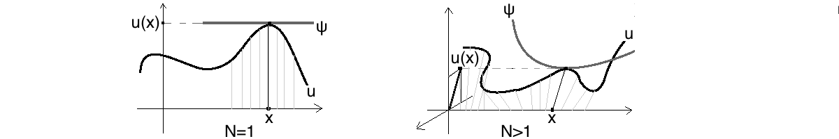 Figure 0
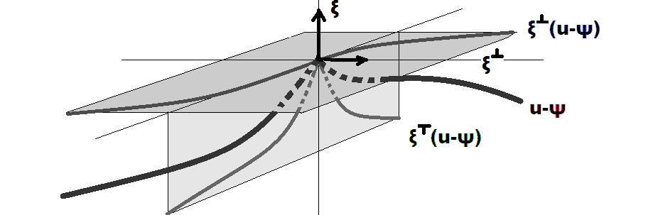 Figure 1
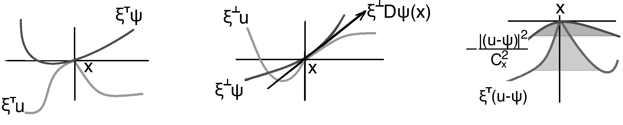 Figure 2
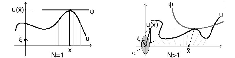 Figure 3
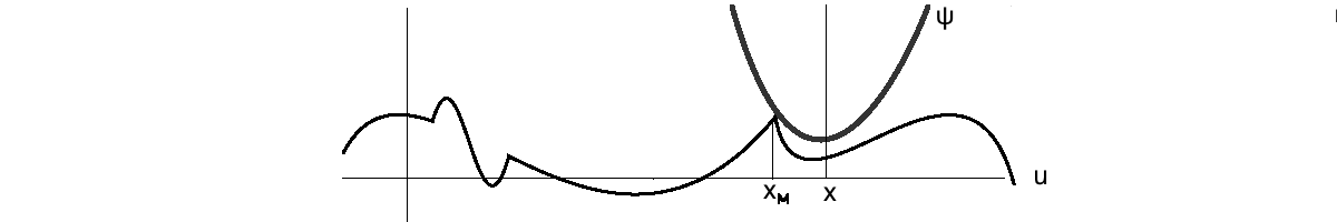 Figure 4
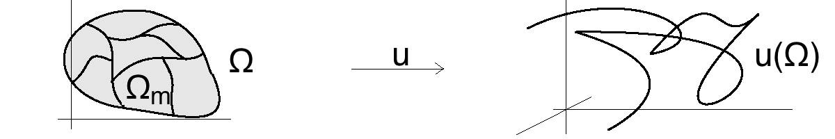 Figure 5
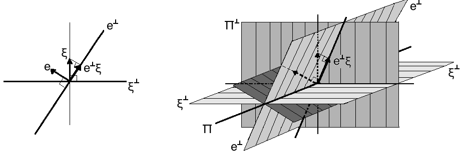 Figure 6
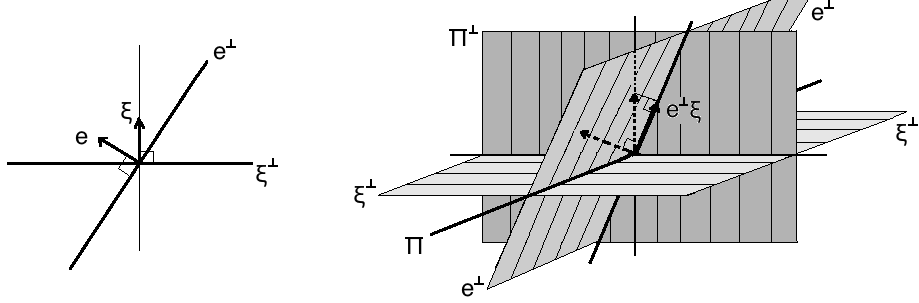 Figure 6
Peer Reviews
No public reviews on file for this paper yet. If you reviewed it on a platform where reviews are public (OpenReview, ICLR, NeurIPS, ICML), you can paste yours below so the community can read it here.
Videos
No videos yet. Explain this paper in a talk, walkthrough, or lecture? Add one.
On a vector-valued generalisation of viscosity solutions for general PDE systems
Nikos Katzourakis
Department of Mathematics and Statistics, University of Reading, Whiteknights, PO Box 220, Reading RG6 6AX, United Kingdom
Abstract.
We propose a theory of non-differentiable solutions which applies to fully nonlinear PDE systems and extends the theory of viscosity solutions of Crandall-Ishii-Lions to the vectorial case. Our key ingredient is the discovery of a notion of extremum for maps which extends min-max and allows “nonlinear passage of derivatives” to test maps. This new PDE approach supports certain stability and convergence results, preserving some basic features of the scalar viscosity counterpart. In this introductory work we focus on studying the analytical foundations of this new theory.
Key words and phrases:
Fully nonlinear PDE systems, degenerate elliptic equations, VS, generalised solutions, maximum principle, extrema, jets
The author has been partially financially supported by the EPSRC grant EP/N017412/1
Contents
- 1 Introduction
- 2 Preliminaries, multilinear maps, tensor inequalities
- 3 Contact solutions for fully nonlinear PDE systems
- 4 Basic calculus of generalised derivatives
- 5 Ellipticity and consistency with classical notions
- 6 The finer structure of contact jets
- 7 The extremality notion of contact maps
- 8 Approximation and stability of contact jets
1. Introduction
The theory of viscosity solutions (VS) of Crandall-Ishii-Lions is one of most successful contexts of generalised solutions in which fully nonlinear degenerate elliptic and parabolic equations can be studied effectively [1, 2, 3, 4, 8, 10, 11, 12, 14, 13, 15, 16, 17, 19, 20, 22, 23, 24, 25, 30, 32]. Main attributes of this approach are the flexibility in passing to limits and the strong uniqueness theorems that supports, albeit the solutions may be nowhere differentiable in any sense.
The tremendous success of VS in the last forty years in tackling a variety of problems has led many researchers to investigate possible generalisations of this theory to virtually any possible direction. Here “generalisation” is meant either in the strict sense of either generalising the main ideas in order to apply under weaker assumptions to more equations, or in the loose sense of generalising the spirit of applicability of this approach. Without being exhaustive, some notable extensions of viscosity solution in either sense are given in [5, 6, 7, 11, 18, 21, 28, 29, 31].
It appears that the main restriction which to date has been unable to be removed is that VS apply to single equations with scalar-valued solutions, or at best to weakly coupled monotone systems which essentially can be treated component-wise as independent equations. Removing this constraint is hardly a straightforward task, as VS are essentially based on the scalar nature of the problem and on comparison arguments through the Maximum Principle and what is typically referred to as its “calculus”, by which is meant that at a point of local extremum of a twice differentiable scalar function, its gradient vanishes and its hessian has sign.
In this work we propose a vectorial generalisation of VS which applies to non-monotone fully nonlinear systems. Our key ingredient is the discovery of a notion of extremum for mappings which extends min/max and allows “nonlinear passage of derivatives” to test maps. This notion of vectorial extremum, which is of independent interest in itself, is coined contact and the term is inspired by the terminology of “touching” by smooth test functions from above/below in the scalar theory of VS. The notion of contact is characterised uniquely by a “maximum principle” type of calculus (vanishing gradient, inequality for the hessian) for vector-valued functions. The notion of contact of maps allows to develop a theory of generalised solutions for systems, coined contact solutions (CS), which supports various stability and convergence results, preserving some of the trademark attributes of VS and in some cases extending mutatis mutandis some well-known scalar facts.
Despite simple to state, the notion of contact presents unfamiliar peculiarities. The possible vectorial “twist” forces the notion to be functional rather than pointwise, in the sense that extremals are maps and not points. Further, it is not associated with any partial ordering. Moreover, it has order: first order contact of two regular maps implies equality of their gradients and second order contact implies an additional certain tensor inequality for their hessians at the point of contact. Finally, it is not very easy to motivate how it arises, as its introduction is justified merely by the generalised maximum principle calculus it carries. Hence, for pedagogical reasons we have chosen to found our exposition on the conceptually equivalent notion of contact jets, rather than contact maps. The former are sets of pointwise generalised derivatives which extend the sub/super jets of VS and vectorial extrema appear rather later in our exposition. We hope that this significantly simplifies the presentation, as contact jets bear a strong formal resemblance with their scalar counterparts in their philosophy, once one replaces the usual inequalities in the Taylor expansions by appropriate tensor inequalities.
One of the first natural question that comes to mind of the experts of VS every time an extension of the notion appears is “what kind of uniqueness results can be obtained”. In the general vectorial case this may not be the right question to ask, but rather “what kind of existence results can be obtained”. For instance, there are striking examples of systems whose scalar counterparts have a good (existence and) uniqueness theory, whilst in the full vectorial case even determining conditions for existence is a highly non-trivial issue (see e.g. [26]). Hence, there are serious limitations due to vectorial obstructions and in this work there is a natural shift towards tools for existence rather than uniqueness.
We now give a brief outline of the contents of this work. In Section 2 we introduce the preliminaries of multilinear algebra required to deal with the vectorial case. In Section 3 we introduce the notion of contact jets as sets of generalised pointwise derivatives and the notion of CS. In Section 5 we introduce the appropriate notion of degenerate ellipticity for fully nonlinear second order systems of PDEs that guarantee the compatibility of CS with classical solutions. In Section 4 we study the basic properties of contact jets, relate them to classical derivatives and prove the compatibility of CS with the classical notions. We also derive some equivalent formulations. In Section 6 we study the local structure around a point at which a contact jet exists. The main result here is a formulation of contact jets which involves a single scalar (not tensorial) fundamental inequality. We then deduce that obstructions arising in the vectorial case imply that the -theory requires a priori little Hölder space regularity and the -theory requires a priori Lipschitz regularity. In the scalar case all obstructions disappear and the reduced theory of semi-jets applies successfully to merely functions. Roughly speaking, in the general vectorial case only “” of the derivatives can be interpreted weakly, the rest “” must exist classically. In Section 7 we present the extremality notion of contact, establish its characterisation through a certain Calculus. Finally, in Section 8 we prove a stability result for contact solutions as an existence tool.
We close this introduction by noting that due to considerations of size and length, in this paper we only introduce and study the abstract rudiments of CS, leaving concrete applications to specific systems for future developments.
2. Preliminaries, multilinear maps, tensor inequalities
Preliminaries. Let . In what follows, will always denote the space of column vectors equipped with the inner product and will stand for the space of matrices equipped with inner product . The respective norms will always be the Euclidean ones , . The unit open ball of centred at will be denoted by and the respective unit sphere by . If , then , will be denoted by , . If , the sign of is if and . The summation convention will always be employed when repeated indices appear in a product and repeated free indices will be denoted with a hat . We henceforth reserve the letters for the dimensions of and ; Greek indices , , ,… will always run from to and Latin , , ,… from to . We denote the space of linear maps by or by and the space of linear maps by . The spaces of linear symmetric/positive endomorphisms of will be symbolised by the respective subscripts “”. Let now be a twice differentiable map. will always denote an open subset and “once” or “twice” differentiability is understood as existence of first or second order Taylor expansions. We view the gradient matrix and the hessian tensor as maps
[TABLE]
where , and , denote the standard bases of and respectively. We also introduce the following contraction operation for tensors which extends the Euclidean inner product of . Let “” denote the -fold tensor product. If , and , we define a tensor in by
[TABLE]
For example, for and , the tensor of (2.3) is a vector with components with free index and the indices are contracted. In particular, in view of (2.3), the second order linear system
[TABLE]
can be compactly written as , where the meaning of “” in the respective dimensions is made clear by the context. Let now be linear map. We will always identify linear subspaces with orthogonal projections on them. Hence, we have the split where and denote range of and nullspace of respectively. In particular, if , then is (the projection on) the line and is (the projection on) the normal hyperplane .
Symmetrised tensor products. The next notion plays a crucial role to what follows. The symmetrised tensor product is the operation
[TABLE]
Obviously, and . Let us also record the identities
[TABLE]
We will also need to consider tensor products “” of higher order between and the spaces and . If , , we view the tensor products and as maps . This allows to define
[TABLE]
Obviously, and . Similarly, if , we view and as maps and we set
[TABLE]
Once again we note that and that . Moreover, since , the tensor is in : indeed,
[TABLE]
Tensor Inequalities and orderings. Let . The latter space comes equipped with its natural ordering
[TABLE]
We now introduce a weaker notion of partial ordering in which emerges in the PDE theory that follows.
Definition 1** (Rank-One Positivity).**
Let . We say that the 4th-order tensor is rank-one positive when the quadratic form is rank-one convex on , that is when
[TABLE]
In this case, we write
[TABLE]
As usually, we define and . We recall the well-known fact that the quadratic form is rank-one convex when the next function is convex on for all , , :
[TABLE]
We now establish that rank-one positivity “” defines a partial ordering in the subspace of consisting of separately symmetric fourth-order tensors:
Lemma 2**.**
Let , , be in . Then:
(i) We have . Also, if , then .
(ii) If , then
[TABLE]
Corollary 3** ( partially orderings).**
The inequality of rank-one positivity defines a partial ordering in the next space of separately symmetric tensors
[TABLE]
Proof of Lemma 2. (i) is trivial. To see (ii), let , . By assumption, we have . Hence,
[TABLE]
If we set , then (2.17) says
[TABLE]
for all , and moreover, by the symmetries of , we have :
[TABLE]
Hence, (2.18) implies for all and all that
[TABLE]
By interchanging in (2.20) and and employing that , we have
[TABLE]
By (2.20) and (2.21), for all fixed we have
[TABLE]
Since \big{(}\Xi_{\alpha i\beta j}+\Xi_{\beta i\alpha j}\big{)}e_{\alpha}\otimes e_{\beta} belongs to , we obtain (2.15) as desired. ∎
Remark 4**.**
It is evident that is a proper subspace of and that it can be equipped with both partial orderings “” and “”. It also evident that “” is a stronger notion than “”, in the sense that implies . The known examples of rank-one convex quadratic form which are not convex imply that rank-one positivity is genuinely weaker that positivity.
3. Contact solutions for fully nonlinear PDE systems
In this section we introduce the basics of a theory of non-differentiable solutions which applies to fully nonlinear systems of partial differential equations of the form
[TABLE]
where and
[TABLE]
The arguments of the nonlinearity will be denoted by \mathrm{F}\big{(}x,\eta,\mathrm{P},{\bf X}\big{)}. For the moment, the only assumption that needs to be imposed to is mere local boundedness. Hence, we allow for discontinuous coefficients. Later we will assume continuity and an appropriate notion of ellipticity, in order to assure compatibility of generalised and classical solutions. Our notion of solution allows to interpret merely continuous maps as solutions to the PDE system (3.1). The point of view is to relax and to certain generalised pointwise derivatives and relax equality in (3.1) to appropriate inequalities, when is evaluated at these generalised derivatives.
Definition 5** (Contact jets).**
Let be a continuous map, and . The first contact -jet of at is the set of generalised derivatives
[TABLE]
The second contact -jet of at is the set of generalised derivatives
[TABLE]
Remark 6**.**
The meaning of “” in (5), (5) is that there exists a continuous matrix-valued map such that as . The meaning of the rest quantities appearing is that given in formulas (2.5)-(2.9). In particular, matrix inequalities are considered in . The necessity to define generalised derivatives on boundary points of closed sets stems from the necessity to consider boundary value problems for PDE systems, but also for technical reasons arising in our subsequent analysis. If , since is open the statement “” which means “convergence in ” can be dropped.
In the scalar case of , we have and , reduce to the semi-jets and of VS. Indeed, for any and (5) reduces to inequality in . Moreover, by applying “” to (5) we deduce that the “scalar” -projection of along satisfies , and similarly for (5) (see (2.6)).
In the following we will also need to consider closures of contact jets:
Definition 7** (Contact jet closures).**
Let be a continuous map, and . The first contact -jet closure of at is
[TABLE]
The second contact -jet closure of at is
[TABLE]
The main difference of (7), (7) compared to their scalar counterparts is that we approximate in the direction as well. When no such option is available, since is totally disconnected. Before giving our notion of solution, we need one more definition, which we state only for the second order case.
Definition 8** (Envelopes of discontinuous coefficients).**
Given and consider the map of (3.2) which we assume is locally bounded. The -Envelope of is the upper semi-continuous envelope of the projection :
[TABLE]
We now proceed to the main notions of solutions we will use in this work.
Definition 9** (Contact solutions for second order systems).**
Consider the map of (3.2) and suppose it is locally bounded. The continuous map is called a contact solution to (3.1) on when for any and we have
[TABLE]
Similarly, one can specialise the notion for first order systems as follows.
Definition 10** (Contact solutions for first order systems).**
Suppose the map
[TABLE]
is locally bounded. The continuous map is called a contact solution to
[TABLE]
on , when for all and we have
[TABLE]
Remark 11**.**
We observe that for , CS reduce to viscosity solutions (up to a difference in the sign convention in the inequality). However, the new ingredients in the contact notions which are not component-wise will lead to genuinely vectorial phenomena.
The new objects , will be studied thoroughly later. Before presenting some explicit calculations of contact jets for a typical map to illustrate the working philosophy (which is analogous to the scalar case), we present a reformulation of Definitions 9-10.
Lemma 12** (Alternative definitions).**
In the setting of Definitions 9-10, the implications (3.11), (3.8) can be respectively replaced by
[TABLE]
If moreover the nonlinearity is continuous, we can replace the by .
Proof of Lemma 12. For brevity we exhibit only the second order case. Obviously, . Conversely, assume (3.13) and fix . Then, there is a sequence as and also . By (3.13) and since is continuous and is locally bounded, there exists a bounded open set centred at such that
[TABLE]
for large. Since is upper semi-continuous, by letting we obtain that . Hence, the map is a contact solution. ∎
4. Basic calculus of generalised derivatives
In this section we examine the pointwise generalised derivatives and and relate them with the classical ones . We begin with two simple algebraic results will turn out to be essential tools.
Lemma 13** (Spectral decomposition of symmetrised tensor products).**
Let and . Then, is a symmetric matrix with rank at most and its the spectrum of consists of at most three distinct eigenvalues , given by
[TABLE]
The respective eigenspaces are
[TABLE]
Proof of Lemma 13. If or is co-linear to , the result is obvious. If are linearly independent, we observe that \mathrm{N}\big{(}\xi\vee R\big{)}=\left(\mathrm{span}[\{\xi,R\}]\right)^{\bot}: indeed, for all , we have the identity
[TABLE]
Hence, is normal to both and if and only if . By the Spectral Theorem, has at most three distinct eigenvalues ,[math], and
[TABLE]
We now employ (4.3) to check directly that
[TABLE]
with as in (4.1). The lemma follows. ∎
We now show that symmetric products coupled by the inequality induce “directed” orderings.
Proposition 14** (Induced partial orderings).**
Let be in and .
(i) If , then
[TABLE]
(ii) If , then
[TABLE]
In particular, it follows that the orderings and coincide on the cone
[TABLE]
which is a subspace of the space (2.16) of separately symmetric tensors.
Proof of Proposition 14. (i) By Lemma 13, if and only if , hence if and only if and this says . The latter is equivalent to with and to with .
(ii) Suppose that and fix and . Then, we have
[TABLE]
By (4), we obtain for any fixed that . By employing (i) to the vector , we see that
[TABLE]
for any fixed. Since is arbitrary, we obtain the desired decomposition which can be recast as , . Finally, by assuming the latter decomposititon and fixing , we have
[TABLE]
and the last inequality follows by . Hence, as desired. Finally, the implication is trivial. ∎
Now we relate generalised and classical pointwise derivatives.
Theorem 15** (Contact jets and derivatives).**
Let be a map which is continuous at .
(a) If there exists one direction such that both are nonempty, then is differentiable at and both are singletons with element the gradient:
[TABLE]
(b) If is differentiable at , then for all the sets are singletons with element the gradient:
[TABLE]
Moreover, whenever , we have the inequality
[TABLE]
which is equivalent to
[TABLE]
(c) If is twice differentiable at , then for all the sets are nonempty, they contain and also
[TABLE]
Moreover, we have the characterisations
[TABLE]
(d) If is twice differentiable at and , then
[TABLE]
Proof of Theorem 15. (a) Let . Then, by (5), we have
[TABLE]
if , where “” is realised by . We set for and fixed and add the inequalities in (4.29) to obtain
[TABLE]
as . By taking the limit to (4.30) and then replacing with , we obtain \xi\vee\big{[}(\mathrm{P}^{+}-\mathrm{P}^{-})w\big{]}:\eta\otimes\eta=0. By applying Proposition 14, we find that vanishes. By Lemma 13, we obtain that zero is the unique eigenvalue of , that is, \sigma\big{(}\xi\vee(\mathrm{P}^{+}-\mathrm{P}^{-})\big{)}=\{0\}. Hence, we have
[TABLE]
for any . As a result we get . Let us denote their common value by . Then, by (4.29) we have
[TABLE]
as . Since the numerical radius (cf. [27])
[TABLE]
is a norm on equivalent to the Euclidean, (4.32) implies as that
[TABLE]
for some . By applying (2.7), (4.34) gives
[TABLE]
as . Consequently, we have and J^{1,\xi}u(x)=\big{\{}\mathrm{D}u(x)\big{\}}.
(b) If is differentiable at , by applying to the Taylor expansion which holds as , we discover \big{\{}\mathrm{D}u(x)\big{\}}\subseteq J^{1,\xi}u(x), for any . Since then both , application of (a) implies that J^{1,\xi}u(x)=\big{\{}\mathrm{D}u(x)\big{\}}. Let . By (5), we have
[TABLE]
as . Hence, (a) implies that whenever and is differentiable. If , we have as
[TABLE]
We set for , and add the inequalities in (4.36) to find
[TABLE]
as , for all . By passing to the limit in (4.37) we obtain
[TABLE]
for all , . Hence, by Definition 1 we obtain \xi\vee\big{(}{\bf X}^{-}-{\bf X}^{+}\big{)}\leq_{\otimes}0. By Proposition 14, the equivalence of the rank-one inequality with (4.22) follows.
(c) We first observe that by applying Proposition 14, all four sets appearing in the right hand sides of of (4.23), (15) are equal. Hence, it suffices to prove that equals one of those. By applying to the Taylor expansion
[TABLE]
which holds as , we find that for all . By applying (b) for and , we obtain the inclusion
[TABLE]
For the reverse inclusion, let us assume that \xi\vee\big{[}\mathrm{D}^{2}u(x)-{\bf X}\big{]}\leq_{\otimes}0. Then by applying to (4.38), we have
[TABLE]
as . By (4), we obtain
[TABLE]
as . Hence, .
(d) follows easily by arguing similarly as in (a), (b), (c). ∎
The next lemma is an essentially scalar fact which will allow to formulate equivalent definitions of , . For the proof we refer to [24].
Lemma 16**.**
Suppose is a continuous symmetric tensor map satisfying as . Then, there exists an increasing function with such that , as .
Now we derive equivalent formulations of contact jets. We shall consider only the case on ; analogous results hold for , with the obvious modifications. For simplicity we fix .
Proposition 17** (Equivalent formulations of ).**
Suppose is continuous at and let and . The following are equivalent:
(a) .
(b) There exists increasing with such that, as
[TABLE]
(c) We have
[TABLE]
(d) We have as that
[TABLE]
(e) We have as that
[TABLE]
Note that for we recover known properties of scalar semi-jets . In particular, reduces to differentiability of the positive part \big{(}u(z)-u(0)-\mathrm{P}z-\frac{1}{2}{\bf X} :z\otimes z\big{)}^{+}. The proof of proposition 17 is very simple and therefore we omit it.
The following simple properties of , are in complete analogy with the scalar counterparts , and are a direct consequence of Proposition 17.
Proposition 18**.**
Let be continuous at and let .
(a) Both , are convex subsets of and respectively.
(b) is closed in . Moreover, for any , the “slice”
[TABLE]
is closed in .
(c) If , then it has infinite diameter. Moreover,
[TABLE]
Proof of Proposition 18. (a) is obvious. For (b), it suffices to establish that the set (4.46) is closed, since the other is similar. Let and as . Fix . Then, there is an such that . By Proposition 17, we have as
[TABLE]
By passing to the limit in (4) and letting , we obtain , as a result of Theorem 17. Finally, for any , , we have
[TABLE]
Consequently, (4.47) follows. ∎
Lemma 33 at the end of Section 6 supplements Proposition 18 by showing how we can modify the contact jet along directions perpendicular to , that is, when we can add to elements of the form for . Now we give an explicit concrete example of jets.
Example 19** (Calculation of contact jets, cf. [24]).**
Let be given by
[TABLE]
where , . The contact jets of at zero are
[TABLE]
where
[TABLE]
The proof of the above facts follows by a simple but lengthy computation by using directly the definition of contact jets.
5. Ellipticity and consistency with classical notions
Now we introduce the appropriate notion of ellipticity for fully nonlinear second order PDE systems and establish compatibility between classical and CS.
Definition 20** (Degenerate elliptic second order systems).**
Let be a map. The PDE system (3.1) is called degenerate elliptic when for all the map is monotone, in the sense that the following matrix inequality holds
[TABLE]
for all , , namely
[TABLE]
By restricting (5.1) to the cases of and of , we recover standard monotonicity notions which (5.1) extends to the general case. If then (5.1) reduces to the standard ellipticity of VS up to a change of sign depending on the convention (see e.g. [14])
[TABLE]
If , then (5.1) reduces to the standard monotonicity of maps . We now derive a characterisation of Definition 20 which is the form of ellipticity we will actually employ in our analysis.
Lemma 21**.**
Let . Then, the following are equivalent:
(i) For all and all , , we have
[TABLE]
(ii) For all , , we have
[TABLE]
Proof of Lemma 21. By Proposition 14, (5.3) is equivalent to
[TABLE]
Assuming (5.5), we have and and also \xi^{\top}\big{(}\mathrm{G}({\bf X})\,-\,\mathrm{G}({\bf Y})\big{)}\leq 0. These relations yield
[TABLE]
Hence, we obtain (5.4). Conversely, assuming (5.4) and that , by Proposition 14 we have and hence we get
[TABLE]
Since , we deduce that , as claimed. ∎
The main result of this section is that CS and classical solutions are compatible for fully nonlinear second order systems which are degenerate elliptic and have continuous coefficients.
Theorem 22** (Consistency).**
Let be a continuous map and consider second order system (3.1).
(a) If is a contact solution of (3.1) and the nonlinearity is continuous, then solves (3.1) classically at points of twice differentiability.
(b) If is a twice differentiable solution of (3.1) and the nonlinearity is degenerate elliptic, then is a contact solution of (3.1).
Proof of Theorem 22. (a) If is a contact solution of (3.1), then, in view of Theorem 15, if is twice differentiable at we have that for any . Hence, by Lemma 12, we have
[TABLE]
Since is continuous, -envelopes coincide with -projections and we obtain
[TABLE]
for all . Since is arbitrary, we deduce that solves (3.1) classically.
(b) Suppose is a twice differentiable solution of (3.1) and satisfies (5.1). Then, if , by Theorem 15 we have and moreover \xi\vee\big{(}\mathrm{D}^{2}u(x)-{\bf X}\big{)}\leq_{\otimes}0. By applying Lemma 2, it follows that whenever ,
[TABLE]
Thus, (5) and Lemma 12 imply that is a contact solution of (3.1). ∎
A particular important class of second order PDE systems to which the theory applies (and has partly been motivated by) is that of quasilinear ones in non-divergence form. For
[TABLE]
the general form of such systems is
[TABLE]
(cf. (2.3), (2.4)). According to the next Lemma, in the quasilinear case of (5.11) the condition of degenerate ellipticity is equivalent to the rank-one positivity of . The latter is the (weak) Legendre-Hadamard condition, when is symmetric, namely when .
Lemma 23**.**
Suppose that . Then, the linear map from to is monotone if and only if .
We note that symmetry of is not required for this equivalence.
Proof of Lemma 23. The monotonicity of reads \big{(}A:{\bf X}\big{)}^{\top}{\bf X}\geq 0. Let us fix , and set . Then, we have
[TABLE]
Hence, . Conversely, if for all and all , we suppose that for some . Then, by Proposition 14 we have where . If is the symmetric square root of , then we have that . Hence, is a sum of positive matrices with . Hence, we have
[TABLE]
and therefore \xi^{\top}\big{(}A:{\bf X}\big{)}\leq 0. By Lemma 21, the map is monotone. ∎
Now we construct a large class of fully nonlinear systems which satisfies the ellipticity condition (5.1).
Example 24** (Fully nonlinear degenerate elliptic systems).**
For any nonlinearity with components of the form
[TABLE]
such that is odd and each is homogeneous and increasing for all indices , the next system is degenerate elliptic:
[TABLE]
The claim above follows by the next result.
Lemma 25** (Monotone functions of the eigenvalues of the hessian).**
Suppose that is odd with each component homogeneous. Suppose further each function is increasing, for all indices . Consider
[TABLE]
where and \big{\{}\lambda_{1}(X_{\alpha}),...,\lambda_{n}(X_{\alpha})\big{\}} denotes the eigenvalues of , placed in increasing order. Then, is monotone in the sense of (5.3).
Proof of Lemma 25. Fix , , , an index and suppose that \xi\vee\big{(}{\bf X}-{\bf Y}\big{)}\leq_{\otimes}0. Then, we have
[TABLE]
where denotes free index (no summation). Hence, we obtain . Since the -eigenvalue function is odd and homogeneous, we have , for any and each . Since each is increasing in each of its arguments, we get
[TABLE]
Since is homogeneous and odd, we obtain
[TABLE]
By summing with respect to , we obtain \xi^{\top}\big{(}\mathrm{G}({\bf X})-\mathrm{G}({\bf Y})\big{)}\leq 0. ∎
Following [14], we can give numerous explicit fully nonlinear degenerate elliptic examples. In particular, the choices , , and lead for any to the systems
[TABLE]
which are fully nonlinear and degenerate elliptic for any first order nonlinearity .
6. The finer structure of contact jets
In this section we study the structure of contact jets more deeply and demystify the local structure of maps around the point at which a contact jet exists. The principal results are Theorems 26-27, which reformulate the matrix inequality defining jets to an ordinary inequality coupling the -projection and the length of the projection on the hyperplane normal to . The inequality connects a semi-differentiability condition for (known from the scalar case) to a new partial regularity condition in codimension-one for the perpendicular part .
Theorem 26** (Structure of first contact jets).**
Let be continuous. Let also , and . Then, the following are equivalent:
(i) .
(ii) There exists an increasing with , such that as
[TABLE]
Theorem 27** (Structure of second contact jets).**
Let be continuous. Let also , and . Then, the following are equivalent:
(i) .
(ii) There exists an increasing with , such that as
[TABLE]
By (6.1) and (27) we obtain that the existence of nontrivial contact jets implies a local structure for the map: the codimension-one projection of on the hyperplane must be more regular than the projection . Actually there is a bootstrap of regularity between and , which balances at differentiability:
Corollary 28** (Codimension-one bootstrap regularity imposed by jets).**
Suppose that is a continuous map, , .
(1) Let and . Then
[TABLE]
as , for any . In particular, for the following holds: since is at , is near . If is differentiable at , then so is .
(2) Let and . Then
[TABLE]
as ,for any . In particular, for the following hold: since is at , is near . If is twice differentiable at , so is .
Proof of Corollary 28. We rewrite (6.1) and (27) as
[TABLE]
and the desired conclusions readily follow. ∎
The fact of existence of nowhere improvable Hölder functions implies
Corollary 29**.**
For any , there exists a map such that does not possess nontrivial first -jets anywhere. Similarly, for any , there exists a map such that \big{\{}x\in\mathbb{R}^{n}\ |\ J^{2,\xi}u(x)\neq\emptyset\big{\}}=\emptyset.
Hence, obstructions arising in the vectorial case imply that first contact jets are efficient for Hölder maps and second contact jets are efficient for Lipschitz maps. In the scalar case obstructions disappear and semi-jets are efficient for merely functions. We interpret this fact by saying that “in the vectorial case only of the derivatives can be interpreted weakly, the rest must exist classically”.
In order to prove Theorems 26-27, we need a technical tool. Let and . By Lemma 13, the tensor product is a rank-two symmetric tensor.
Lemma 30** (Representations of the spectrum of symmetrised tensor products).**
For any , set s(R):=\ 2\big{(}\operatorname{sgn}(\xi^{\top}R)\big{)}^{+}-1. Then, we have the identities
[TABLE]
Proof of Lemma 30. By observing that for any , we have
[TABLE]
we obtain that s(R)=\big{(}\chi_{(0,\infty)}-\chi_{(-\infty,0)}\big{)}(\xi^{\top}R). We assume , since (6.5) is trivial if . Let denote the right hand side of (6.5). Then, we compute
[TABLE]
which gives , as a result of Lemma 13. This establishes (6.5). Let us now establish (6.6). The elementary identity
[TABLE]
implies that
[TABLE]
By comparing (6.5) and (6), we see that (6.6) follows. ∎
The following is the first step towards Theorems 26, 27.
Theorem 31** (Equivalent formulations of contact jets).**
Let be continuous, , , . Let also . Then, the following statements are equivalent:
(i) , that is, as .
(ii) We have
[TABLE]
(iii) There exist maps and satisfying that and as and also
[TABLE]
(iv) If we set T:=\big{\{}|\xi^{\bot}R|\leq|\xi^{\top}R|\big{\}}\subseteq\overline{\Omega}, then
[TABLE]
We observe that when , then and we recover a single inequality along which coincides with that of scalar semijets.
Proof of Theorem 31. We begin by proving that (i) is equivalent to (ii). If we assume (i), then by the representation formula (6.5), it is equivalent to
[TABLE]
as . By (6.12), we have \big{|}R-|R|s(R)\xi\big{|}(z)\leq o\big{(}|z|^{p}|R(z)|^{\frac{1}{2}}\big{)}, as . Hence, there exists an with such that
[TABLE]
on . By projecting (6.13) onto , we obtain on . We set . Therefore
[TABLE]
as . By (6.12) and (6.14), (ii) follows. Conversely, assume (ii). It suffices to verify that as . Then, we calculate
[TABLE]
Since , we have that
[TABLE]
as . Since on we have 1\leq\big{(}|R|+\xi^{\top}R\big{)}/|R| and on we have 1\leq\big{(}|R|-\xi^{\top}R\big{)}/|R|, we infer that
[TABLE]
as . Thus, (6.9) and (6.20) imply (6.12), which is equivalent to (i). Let us now prove the equivalence between (ii) and (iii). If we assume (ii), we define
[TABLE]
It follows that , have the desired properties and by (6.21), we have . It follows that is the positive solution of the quadratic equation . Hence,
[TABLE]
Thus, (6.21) and (6.22) imply (6.10). Conversely, if we assume (iii) and let be defined by the formula giving above, then solves the equation . Hence, by the above and perpendicularity, we have
[TABLE]
This, and hence . As a result, (6.10) implies (6.9) as claimed. We conclude by proving that (iv) is equivalent to (ii). For, let us split as and equip it with the norm \|R\|:=\max\big{\{}|\xi^{\top}R|,|\xi^{\bot}R|\big{\}}. Then, we have
[TABLE]
By the above and norm equivalence on , (6.9) is equivalent to
[TABLE]
Since on we have as , (6.25) is equivalent to (6.11) and the theorem follows. ∎
Proof of Theorem s 26, 27. By Theorem 31, it suffices to prove the following:
Claim 32**.**
If is continuous, , , , then
[TABLE]
as , for some increasing which satisfies .
To this end, assume . Then, by Theorem 17, there exists an increasing with as such that
[TABLE]
Let be an orthonormal base of the hyperplane . Then, and the identity can be written as:
[TABLE]
By plugging (6.28) into (6.27), we obtain
[TABLE]
By applying “” to (6.29) and employing orthonormality of the base, we infer that . Let now and be fixed and apply again “” to (6.29) to obtain
[TABLE]
By orthogonality of the base, we deduce that . Since this holds for both , we infer that
[TABLE]
and the choice in (6.30) implies \big{|}\xi_{\beta}^{\top}R\big{|}^{2}\leq 4\rho\big{(}\rho+\xi^{\top}R\big{)}. By summing with respect to , we obtain
[TABLE]
The above estimate implies the direction “” of Claim 32 for the choice . Conversely, assume the validity of the inequality in (6.26) for such a and set . Then, we have
[TABLE]
locally near . Since near zero, (6.31) readily gives as . By setting T:=\big{\{}\big{|}\xi^{\bot}R\big{|}\leq\big{|}\xi^{\top}R\big{|}\big{\}} and \Omega:=\big{\{}\big{|}\xi^{\top}R\big{|}>\rho\big{\}}, the inequality (6.31) implies on that
[TABLE]
as . Hence, by the implication (iv) (i) of Theorem 31, we obtain
[TABLE]
as . On the other hand, on we have \big{|}\xi^{\top}R\big{|}\leq\rho and also \big{|}\xi^{\bot}R\big{|}\leq\big{|}\xi^{\top}R\big{|}, hence by Lemma 13 we estimate
[TABLE]
as . Therefore, we deduce that
[TABLE]
as . Now, by (6.31) on \mathbb{R}^{n}\setminus T=\big{\{}\big{|}\xi^{\top}R\big{|}<\big{|}\xi^{\bot}R\big{|}\big{\}} we have that
[TABLE]
Hence, it holds that \big{|}\xi^{\bot}R\big{|}^{2}-\rho\big{|}\xi^{\bot}R\big{|}-\rho^{2}\leq 0 and by comparing \big{|}\xi^{\bot}R\big{|} with the solutions of the binomial equation , we find
[TABLE]
as . Thus, by employing again Lemma 13, we estimate
[TABLE]
as . By estimates (6.33) and (6.36) we deduce \max\sigma\big{(}\xi\vee R(w)\big{)}\leq o(|w|^{p}) as and consequently . As a result, Claim 32 follows. ∎
The following result certifies that the projections along of second contact -jets are “stiff” and if the map is twice differentiable, no variations can be performed.
Lemma 33**.**
Let be continuous and fix , , and . Then, if , we have
[TABLE]
Lemma 33 says that we can modify by adding an element of the form with along a direction in the normal hyperplane if we can add the element from the superjet of the projection . For modifications along the -direction, see Proposition 18.
Proof of Lemma 33. We set
[TABLE]
By employing that , we estimate
[TABLE]
as . Hence, by assumption we have
[TABLE]
as . By increasing the functions appearing in the summands appropriately, we incorporate the term in the first summand and therefore obtain that , as claimed. ∎
7. The extremality notion of contact maps
So far, our central objects of study have been contact jets, a certain type of generalised pointwise derivatives. Jets in fact introduce in an implicit non-trivial fashion an extremality notion for maps, which we will now exploit. This notion extends min and max of scalar functions to the vector-valued case, effectively extending the “Maximum Principle calculus” ( and at maxima of ) to the vectorial case. This device allows the “nonlinear passage of derivatives to test maps”. This extremality notion, although simple in its form, presents peculiarities and is not obvious how it arises. Hence, we have chosen to base the PDE theory of CS to jets rather than to extrema, since jets seem more reasonable due to the formal resemblance to their scalar counterparts.
Motivation. We begin by motivating the notions that follow. Let be a smooth curve. Every reasonable definition of extremal point at must imply that . However, this is impossible if as the example of unit speed curves certifies for which . In order to succeed we must radically change our point of view of “extremals”. The idea is to relax the pointwise notion to a flexible functional notion of “extremal map” which takes into account the possible “twist”. Our viewpoint is the following: if and has a maximum at , then we can identify the extremum with the constant function which passes through (Figure 1(a)).
[TABLE]
When we can view extrema as maps passing at through which generally are nonconstant (Figure 1(b)).
Going back to , we see that maximum can be viewed as a constant function “touching ” at in the direction and minimum as “touching ” at in the direction . When , there still exists a stiffer notion of “touching ” at by a map in a unit direction . We will call this stronger touching notion contact.
There are two intriguing properties associated with contact which are source of difficulties. Firstly, the notion of contact comprises a notion of extremum not connected to any ordering of (when ). Its main utility is the “nonlinear passage of derivatives to test maps” in our PDE systems. Secondly, the contact has order itself: roughly, “first order contact” implies “gradient equality” and “second order contact” implies an appropriate “hessian inequality”.
To begin, let denote a generic cone function with vertex at and some slope , that is .
Definition 34** (Contact maps).**
Let be continuous and fix and .
(1) The map is a first contact -map of at if and for every cone , there is a neighbourhood of in such that, thereon, we have
[TABLE]
(2) The map is a second contact -map of at if and for every cone , there is a neighbourhood of in such that, thereon, we have
[TABLE]
In Definition 34 we allow for boundary points , but we are mostly interested in interior points . Inequalities (7.1) and (7.2) contain a lot of information. Specifically, (7.2) says that for every , exists an such that
[TABLE]
for . Hence, (7.2) is an elegant restatement of
[TABLE]
as , by using “control by cones”. Since the left hand side of (7.4) is nonnegative and , the projection along the line in spanned by has a (local) vanishing maximum at :
[TABLE]
for near (Figures 2(a), 3).
[TABLE]
Moreover, since the right hand side of (7.4) is of order , the projection along the hyperplane has a vanishing derivative at , since as (Figures 2(b), 3). Hence, since coincides with at , the codimension-one projection on the hyperplane is differentiable and , although * may not exist*.
[TABLE]
Moreover, (7.4) reveals that there is a coupling between and , which can be interpreted as that either the maximum of is constrained by or that the decay of near is controlled by via cones (Figures 2(c), 3).
We will shortly see that contact maps constitute an appropriate notion of extremum for PDE theory. Let us first connect contact maps to contact jets. We will consider only the second order case and and we refrain from providing details for the first order case and boundary points which can be done by simple modifications. Given a continuous , and , set
[TABLE]
Theorem 35** (Equivalence between extremality and jets).**
If is continuous, and , then
[TABLE]
That is, contact jets coincide with the set of derivatives of contact maps.
The proof is based on the following lemma, which roughly states that we can always absorb all of the second order Taylor remainder of a contact -map into its -projection:
Lemma 36**.**
Let be a second contact -map of the continuous map at . There exists a second contact -map of at such that up to second order at (that is, , and ) while the -projection of the second order Taylor remainder of vanishes.
Proof of Lemma 36. Let and denote the operators of second order Taylor polynomial and Taylor remainder at respectively. Then, by (7.2), we have
[TABLE]
locally in a neighbourhood of . By employing Lemma 21 for , we can find an increasing with such that and
[TABLE]
near . By expanding the first term of (7.9), we estimate
[TABLE]
Hence,
[TABLE]
In view of the above, the lemma follows by defining \hat{\psi}:=T_{2,x}\psi\,+\,2\big{(}\rho+|\xi^{\bot}R_{2,x}\psi|\big{)}\xi. Indeed, by construction we have , , and . Moreover, we have \xi^{\top}R_{2,x}\hat{\psi}=2\big{(}\rho+|\xi^{\bot}R_{2,x}\psi|\big{)}\geq\xi^{\top}R_{2,x}\psi. Thus, we infer that
[TABLE]
and since as , for every cone with vertex at , there exists a neighbourhood of such that, thereon,
[TABLE]
We may now establish Theorem 35.
Proof of Theorem 35. Let be a second contact -map of at . By Lemma 36, there exists a second contact -map of as such that up to second order at and moreover . By (7.2), for any , there exists an such that
[TABLE]
whenever . By Lemma 16 for , there exists an increasing function such that and as , and also
[TABLE]
as . By Theorem 27, the above implies \big{(}\mathrm{D}\psi(x),\mathrm{D}^{2}\psi(x)\big{)}\in J^{2,\xi}u(x). Conversely, let . Again by Theorem 27, if is as stated, the map
[TABLE]
satisfies , and
[TABLE]
as . Hence, is a second contact -map of at . The theorem follows. ∎
In view of Theorem 35, we can reformulate Definitions 9-10 of CS as follows (we state only the second order case for brevity):
Definition 37** (Contact solutions for second order systems, cf. Def. 9).**
Suppose is as in (3.1). Then, the continuous map is a contact solution to (3.2) when for any any and any second contact -map of at , we have
[TABLE]
The “contact principle calculus” result we establish below explains why contact maps of the solution play the role of smooth “test maps” for the PDE system.
Theorem 38** (Nonlinear passage of derivatives to contact maps).**
Suppose is a continuous map, twice differentiable at . Let and be given. Consider the following statements:
(i) is a second contact -map of at .
(ii) We have
[TABLE]
Then, (i) implies (ii). Moreover, (ii) implies (i) if moreover \xi^{\top}\mathrm{D}^{2}\big{(}u-\psi\big{)}(x)<0.
Trivial modifications in the arguments of the proof of Theorem 38 that follows readily imply the following consequence.
Corollary 39** (first order contact).**
In the setting of Theorem 38, we have that if is differentiable, then is a first contact -map of at if and only if \mathrm{D}\big{(}u-\psi\big{)}(x)=0.
Theorem 38 has already been established implicitly, in the language of contact jets. Indeed, one may employ Theorem 35 and Proposition 17 to remove the disguise. Further, one can also easily establish the next consequence.
Corollary 40** (Rank-One Decompositions).**
In the setting of Theorem 38, we have that if is a second contact -map of at , we have the rank-one decompositions
[TABLE]
Conversely, if the relations (7.17)-(7.20) hold true, then is a second contact -map of at if in addition the inequality (7.20) is strict.
8. Approximation and stability of contact jets
In this section we consider the problem of stability of CS under limits. We recall that in the scalar case, VS pass to limits under merely locally uniform convergence. This means that if the sequence of solutions to equations satisfies and the nonlinearities satisfy , both convergences locally uniform as , then solves . This important property is a consequence of the fact that maxima perturb to maxima under uniform convergence.
We begin with a counterexample which shows that in the vectorial case this property fails. More precisely, second contact maps do not perturb to second contact maps not even under strong convergence, and neither convergence suffices for any . Moreover, the first order variant of Example 41 below shows that first contact maps do not perturb to first contact maps under convergence for any .
Example 41** (Instability of contact maps).**
For any , there exist , , a second contact -map of at and a sequence such that in and in as , but there exists no sequence of second contact -maps of along any such that \big{(}\mathrm{D}\psi_{m}(x_{m}),\mathrm{D}^{2}\psi_{m}(x_{m})\big{)}\to\big{(}\mathrm{D}\psi(0),\mathrm{D}^{2}\psi(0)\big{)} as .
Indeed, define by , fix and set and . We first verify that is a second contact -map at : for any , there is such that for ,
[TABLE]
which yields \big{|}\xi^{\bot}(u-\psi)(z)\big{|}^{2}\leq\ L^{2}|z|^{2}\big{[}-\xi^{\top}(u-\psi)(z)\big{]}. Consider now the sequence where is the standard mollification of . Since , we obtain that and consequently (a) and (b) follow. Since is smooth, it possesses contact maps at all . Choose a sequence and let be a second contact -map of at . Then, by Corollary 28 we have that is equal up to second order to at . Hence, as we have
[TABLE]
The reason of instability of contact maps is that projections on the normal hyperplane of “generalised hessians” can be the whole tensor subspace . This phenomenon is a general fact, which appears when fails to be near the basepoint. The next lemma exhibits the previous situation and supplements Corollary 28. By utilising this result and the properties of the Little Hölder space which is the closure of under the Hölder norm, it follows that not even convergence suffices (if ).
Lemma 42**.**
Let be a second contact -map of the continuous map at for some . We set:
[TABLE]
If , then, all quadratic perturbations are also contact -maps for any . If , then is unique (up to superquadratic perturbations as ).
Proof of Lemma 42. If , there is with with
[TABLE]
for . Hence, and since is a contact -map, we estimate as
[TABLE]
To see the last claim, apply Corollary 28 and Lemma 36. ∎
Happily enough, the discouraging instability of contact maps is not detrimental to the stability of CS. The reason is that when we try to approximate a system by adding a “viscosity term”, there exists some extra information which is trivial in the scalar case and allows convergence of the approximating solutions. In order to make this statement precise, we introduce an auxiliary notion of sequential derivatives needed in the exploitation of stability and approximation.
Definition 43** (Approximate derivative).**
let be a continuous map. The set of Approximate first jets of at is
[TABLE]
The set of Approximate second derivatives of at is
[TABLE]
Remark 44**.**
Obviously, if is (twice) differentiable at , then and . In general, approximate derivatives may exist at non-differentiability points, as it happens for the Lipschitz continuous function given by for and for which , while does not exist. This follows from the observation .
The following is the main approximation result for contact jets. It follows that contact jets perturb to contact jets under weak∗ convergence in the local Lipschitz space, together with a technical assumption which appears to be satisfied in the cases of interest. This assumption requires convergence of codimension-one projections of sequential jets along a sequence of hyperplanes.
Theorem 45** (Approximation of contact jets).**
Let be continuous and fix for some , . Suppose there exists such that in and for some we have
[TABLE]
Then, there exist sequences and with satisfying and also \big{(}\mathrm{P}_{m},\xi^{\top}{\bf X}_{m}\big{)}\longrightarrow\big{(}\mathrm{P},\xi^{\top}{\bf X}\big{)} as .
Theorem 45 is optimal: by example 41, not even convergence suffices to guarantee . There is a “loss of information” which occurs when (i.e. when ). The proof is based on the next result which relates approximate derivatives of codimension-one projections to contact jets.
Proposition 46** (Approximate derivatives and contact jets on hyperplanes).**
Let be continuous and and . Then, we have:
[TABLE]
In particular, if both sets e^{\bot}\big{(}J^{1,\xi}u(x)\big{)}, are nonempty, they are singletons and coincide. If moreover , then . Further:
[TABLE]
Corollary 47**.**
By (8.6) and Lemma 2, we deduce that on the hyperplane of and along (Figures 6(a),(b)).
[TABLE]
Remark 48**.**
Proposition 46 is optimal, as the example shows: indeed, we have but does not exist, although and coincide and are singletons. Namely, some “loss of information” occurs when (i.e. when ).
Proof of Proposition 46. Since , exists such that
[TABLE]
as , for all . Fix . If , then , and for any , exists with . Since , (8.7) gives
[TABLE]
as . Since , we have
[TABLE]
as . By choosing in (8.9) and summing (8.9) and (8.8), we get (\theta_{\varepsilon}^{\top}\xi)\big{[}\theta_{\varepsilon}^{\top}\big{(}\mathrm{Q}-e^{\bot}\mathrm{P}\big{)}w\big{]}\leq o(1) as . By interchanging with , using that and letting , we get \theta_{\varepsilon}^{\top}\big{(}\mathrm{Q}-e^{\bot}\mathrm{P}\big{)}=0. By letting , we find \theta^{\top}\big{(}\mathrm{Q}-e^{\bot}\mathrm{P}\big{)}=0. Since is arbitrary and , we conclude that . If and moreover , Corollary 28 and Definition 43 imply that . Further, if , it trivially follows that . Since , part (a) implies that . Fix . By arguing as eaelier, there exists such that
[TABLE]
as , for all . By writing for some , using the symmetry of and summing (8.10) and (8.11), we obtain as
[TABLE]
By passing to the limit we conclude that . ∎
Proof of Theorem 45. Since , we have . By the convergence as , standard arguments of the scalar case (see e.g. [14, 24]) imply that there exists and such that
[TABLE]
Since , it follows that and . By Theorem 15, the set contains
[TABLE]
By decomposing , in view of (8.12) and (8.13) we see that it suffices to use (8.4) in order to show that as . For the sequence , assumption (8.4) implies that there exists a convergent sequence of directions and an Approximate jet such that as . Since , Proposition 46 implies that and as a result we deduce that as . Further, by replacing as we can by , we may assume that , namely that lie in the same halfspace (Figures 6(a),(b)). We distinguish two cases:
Case 1: . We use expansions with respect to non-orthonormal coordinates in order to show that as . We define the codimension-two subspaces and which are intersections of hyperplanes (see Figures 6(a),(b)) and allow to write
[TABLE]
Let us now de define the unit vectors and . By expansion on the non-orthonormal frames , , we have that for any , there exists such that
[TABLE]
Since are normal to and , by projecting (8.15)-(8.16) along and we obtain
[TABLE]
By solving the linear system (8.17), we find
[TABLE]
We observe that and use (8.15) and (8.18) to expand as
[TABLE]
By recalling that , we observe that . By using this and that , we rewrite (8.19) as
[TABLE]
Similarly, we have
[TABLE]
By using that , we obtain , as . Also, since and for large enough, we have . Since by assumption , for large we have . Hence, as . By (8.14) we have and hence as . Since and , in view of (8.20), (8.21), it suffices to show that and that as . Indeed we have the estimate
[TABLE]
as , and similarly we conclude that .
Case 2: . If in addition for infinitely many terms , then as and the conclusion follows. If on the other hand for large enough, then the arguments of the previous case fail because we see that . Instead, by using that and , the local weak∗ convergence gives for large enough the bound
[TABLE]
By using (8.22) and that , we estimate
[TABLE]
Since , , and , the bounds (8.22) and (8) allow us to conclude. ∎
The reference list from the paper itself. Each links out to its DOI / PubMed record.
- 1[1] M. Bardi, I. Capuzzo Dolcetta, Optimal Control and Viscosity Solutions of Hamilton-Jacobi-Bellman Equations , Systems & Control, Birkäuser, 1997.
- 2[2] M. Bardi, M.G. Crandall, L.C. Evans, H.M. Soner, P.E. Souganidis, Viscosity solutions and applications , Lecture Notes in Math., vol. 1660. Springer, Berlin, 1997.
- 3[3] G. Barles, Solutions de Viscosité des Équations de Hamilton-Jacobi , Mathématiques et Applications 17, Springer, 1994.
- 4[4] E. N. Barron, Viscosity solutions and analysis in L ∞ superscript 𝐿 L^{\infty} , in Nonlinear Analysis, Differential Equations and Control , Dordrecht 1999, 1 - 60.
- 5[5] G. Bellettini, H. Chermisi, M. Novaga, The Level Set Method for Systems of PD Es , Communications in PDE 32:7, 1043 - 1064 (2007).
- 6[6] K.A. Brakke, The motion of a surface by its mean curvature , volume 20 of Mathematical Notes, Princeton University Press, Princeton, 1978.
- 7[7] R. Buckdahn, J. Ma, Stochastic viscosity solutions for nonlinear stochastic partial differential equations. Part I , Stochastic Processes and their Applications 93 (2001) 181-204 and 205-228.
- 8[8] L.A. Caffarelli, X. Cabré, Fully Nonlinear Elliptic Equations , AMS, Colloquium Publications 45, Providence, 1995.