3-Colorable Delaunay Triangulations
Lucas Moutinho Bueno

TL;DR
This paper introduces an algorithm for constructing a 3-colorable Delaunay triangulation by adding a minimal number of new points to a given set, ensuring the triangulation's colorability.
Contribution
The paper presents a novel algorithm that efficiently produces a 3-colorable Delaunay triangulation with minimal augmentation of the point set.
Findings
Algorithm successfully creates 3-colorable triangulations
Minimizes the number of added points
Applicable to various point configurations
Abstract
We propose an algorithm to create a 3-colorable Delaunay Triangulation. The input of the problem we are trying to solve is a set X of n twodimensional points. The output is a 3-colorable two-dimensional Delaunay triangulation T for X U Y , where Y is a set of m new points. We want to m be as few as possible.
Click any figure to enlarge with its caption.
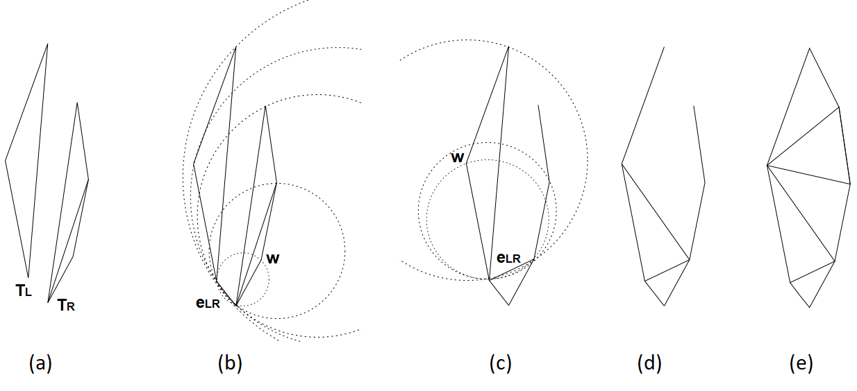 Figure 1
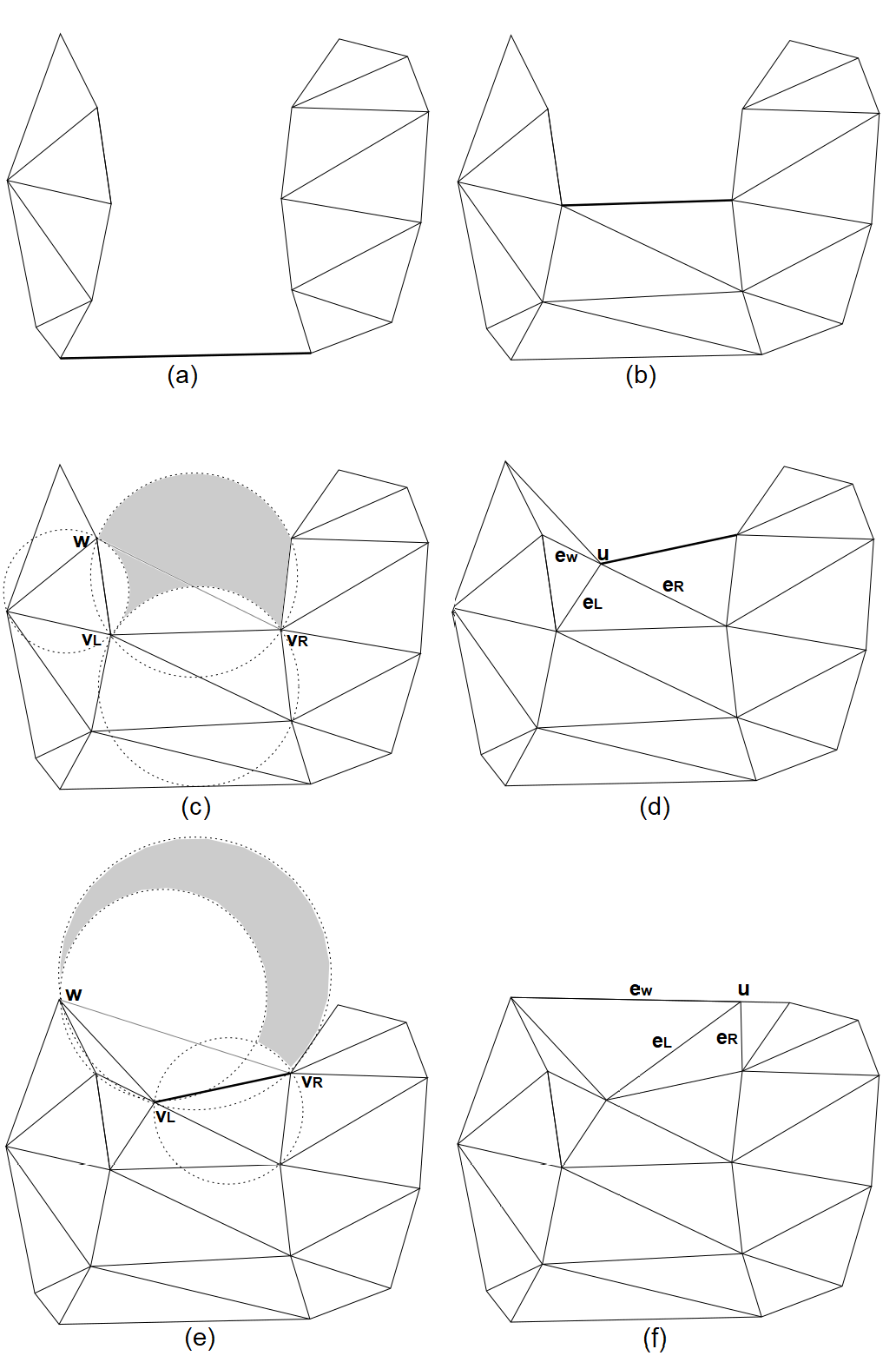 Figure 2
Peer Reviews
No public reviews on file for this paper yet. If you reviewed it on a platform where reviews are public (OpenReview, ICLR, NeurIPS, ICML), you can paste yours below so the community can read it here.
Videos
No videos yet. Explain this paper in a talk, walkthrough, or lecture? Add one.
Taxonomy
TopicsComputational Geometry and Mesh Generation · Data Management and Algorithms · Geographic Information Systems Studies
3-Colorable Delaunay Triangulations
Lucas Moutinho Bueno
Institute of Mathematics and Computer Sciences
University of São Paulo - São Carlos - Brazil
1 Introduction
1.1 Objective
The input of the problem we are trying to solve is a set of two-dimensional points. The output is a 3-colorable two-dimensional Delaunay triangulation for , where is a set of new points. We want to be as few as possible.
1.2 Motivation
Delaunay triangulations are popular triangulations that maximize the minimum angle of all the interior angles of the triangles. This property is desirable for some geometric operations such as interpolation or rasterization.
The adjacency of the triangles in a triangulation might be represented by a data structure. We are particularly interested in using the GEM data structure [1, 2] for this purpose.
This structure is compact and has some operational advantages over others. It is also generalizable to dimensions higher than two. However, it can only represent 3-colorable triangulations , i.e., the triangulations that one can assign one of colors (labels) from to each vertex as long as any two adjacent vertices have different colors.
The GEM data structure represents each triangle by a record with pointer fields , , corresponding to three colors. The field points to the record of the triangle that is adjacent to across the edge opposite to the vertex of color .
Unlike other triangulation data structures, there is no need to identify which side of is the edge , or to perform runtime checks to obtain that information (e.g: from vertex pointers): in the GEM structure points back to .
1.3 Definitions
A pseudo-triangulation (on the plane) is a partition of a compact connected space into sets of vertices (), edges () and triangles ().
A triangulation (on the plane) is a pseudo-triangulation, such that:
- •
Every edge is an open line segment of ;
- •
Every vertex is a point of ;
- •
The endpoints of every edge are vertices of the triangulation;
- •
Every vertex is an endpoint of some edges;
- •
Every triangle is bounded by a cycle of three edges and vertices;
- •
Every edge is on the boundary of one or two triangles;
- •
;
- •
.
An edge that is in the boundary of two triangles is an interior edge, otherwise it is a border edge.
If all edges with a common endpoint are interior edges and is the endpoint of at least one edge, then we say that is an interior vertex, otherwise is a border vertex.
A Delaunay triangulation (DT) is a triangulation where is the convex hull of and where no vertex is inside the circumcircle of any triangle. If there is no subset of with more than three co-circular vertices, then the DT is unique.
An even Delaunay triangulation (EDT) is a triangulation where every interior vertex is even (every interior vertex is the endpoint of an even number of edges).
A locally Delaunay edge is an edge that is either a border edge or there is no vertex inside the circumcircles of both its incident triangles.
An incomplete Delaunay triangulation (IDT) is a pseudo-triangulation where every edge is locally Delaunay.
If is a cycle with four edges and four vertices and is the edge that splits into two triangles, then the flip edge of is an edge that would have the endpoints of different from .
Given a vertex of a triangulation, is the horizontal coordinate of in the Euclidian plane and is its vertical coordinate.
2 Algorithm for 3-colorable Delaunay triangulations
It is known that a two-dimensional Delaunay triangulation is 3-colorable if, and only if, all its interior vertices are even [4]. Therefore constructing a 3-colorable two-dimensional Delaunay triangulation is the same as constructing an EDT.
2.1 Review of the Divide and Conquer algorithm for DTs
Below, we describe the Divide and Conquer Algorithm (DQA) for two-dimensional DT from Guibas and Stolfi [3]. This algorithm is the base to construct an EDT and it runs in time.
The input of the algorithm is a set of two-dimensional points. Its output is a Delaunay triangulation , where .
:
2. 2.
3. 3.
. Return
The procedure sorts the points of into a sequence of vertices in ascending order of the horizontal coordinate.
The procedure splits the sequence of vertices into groups of three consecutive vertices each and one group of two vertices if or a single vertex if . For each group of three vertices, a triangle is created while connecting the vertices with edges. If there is a group of two vertices, an edge is created between them. Each group of vertices, together with its new triangle and edges, is stored as the pseudo-triangulation , for every . Note that is always an IDT. In particular, is a DT for .
The procedure merges IDTs ( to ) into a single DT. The steps of the procedure are described below. It uses the following auxiliaries: three IDTs (left triangulation), (right triangulation) and , five vertices , , , and , and an edge .
:
if then return 2. 2.
if then:
- (a)
2. (b)
3. 3.
Set . Let and be the vertices of and with the lowest vertical coordinate, respectively. Let and be the vertices of and with the highest vertical coordinate, respectively. 4. 4.
Create the edge with endpoints and and add into 5. 5.
while and , repeat:
- (a)
find the vertex from such that there is no vertex from or inside the circle formed by , and 2. (b)
if then else 3. (c)
create the edge with endpoints and , that will form a new triangle ; add and into 4. (d)
remove from and all edges intersecting , together with their incident triangles 6. 6.
Return the triangulation formed by
The proof of correctness of the DQA, in particular the existence and uniqueness of the vertex of Step 5a, can be found in [3]. It is also important to note that during the execution of the Merge procedure, is an IDT.
See Figure 1 for an example of execution of the Merge procedure.
2.2 Making the Triangulation Even
In order to make an EDT, we modify the Merge procedure with the following steps, that are executed just after Step 5a.
- 5a’
if and is odd or if and is odd, then:
- 5a’1
create three edges , and and a vertex as a common endpoint of these edges. Set , and as the second endpoint of , and , respectively. Add , , and into . Two new triangles will be created and also added into . The coordinates of must be chosen in such a way that is an IDT. 2. 5a’2
Let be the vertex of with the lowest horizontal coordinate. If then and , else and . 3. 5a’3
Continue from Step 5.
We will call the new modified procedure as Merge’ and the new modified algorithm as DQA’.
The procedure is similar to the procedure , except for the following items:
- •
The parameter of is replaced by an edge in .
- •
Steps 1 and 2 of are skipped in .
- •
In Step 3 of , and are set to be the endpoints of the edge (one of them will be the vertex , passed as parameter).
- •
The edge won’t be created again in Step 4 but will be included into normally.
In practice, one can see that when is executed, . Therefore, during the execution of the loop (Step 5) and the vertex will always be chosen from the vertices of at Step 5a. Analogously, one can see a similar execution pattern for , by changing by and other related variables.
See Figure 2 for an example of execution of DQA’.
3 Correctness
First of all, note that the vertex of Step 5a’2 of and serves to ensure that, after execution of , all vertices of will have a lower or the same horizontal coordinate than any vertex from , preserving a property needed to function properly, as well as and .
During the execution of DQA’ and, in particular, during the execution of and , one can see that every edge added into can only be added if is an IDT. This is true even for the edge added during Step 4, since it is a border edge and its addition into won’t create any interior edges in . Therefore, assuming that the algorithm is correct, must always be an IDT.
One can also see that all vertices from the input of DQA’ start as border vertices and all vertices created at Step 5a’1 of and are created as border vertices. The Step 5a of and is the only step that turns a border vertex into an interior vertex and Step 5a’1 prevents that vertex to be odd. Therefore, assuming that the algorithm is correct, the interior vertices of must always be odd.
Finally, note that the conditions for ending the loop at Step 5 are the same for , and . Those conditions turn into a triangulation of a convex hull and therefore turn an IDT into a DT. Since the interior vertices of must always be odd, assuming that the algorithm is correct, the final triangulation must be an EDT.
However, we still need to guarantee the existence of the vertex created at Step 5a’1 of and and we still need to guarantee that the creation of new vertices won’t cause the loop at Step 5 to be endless. The lemma below proves half of what we still need.
Lemma 1**.**
During the execution of Step 5a’1 of or , it is always possible to choose coordinates for in such a way that is an IDT.
Proof.
To prove this lemma, we need to guarantee that there are coordinates for where the new interior edge will be locally Delaunay and the former border edges and will remain locally Delaunay after the execution of Step 5a’1.
The new edges and will be locally Delaunay because they will be on the border of . The remaing edges that are not don’t need to be tested because they were already locally Delaunay and won’t change with Step 5a’1.
Let be the edge of with endpoints and , and let be the vertex of opposite from . Analogously, let be the edge of with endpoints and , and let be the vertex of opposite from . We also define as the cycle formed by the vertices , and ; as the cycle formed by the vertices , and ; and as the cycle formed by , and .
We must chose coordinates for in such a way that they won’t be inside nor . Since we want the edge to be in the final triangulation instead of the edge , then must be inside or part of it.
We know that is an IDT. Therefore, is either outside or a point of . Likewise, is either outside or a point of .
Let be the arc of from to . If is a point of , then , , and are cocircular and . Likewise, if is a point of , then . On the other hand, if is outside , then the points of are outside , except for . Likewise, if is outside , then the points of are outside , except for . In any case, since the length of is greater than zero, there is a point of , different from and , that is either outside or part of and/or . Since that point is part of it can be chosen for in such a way that remains an IDT after the execution of Step 5a’1.
∎
Note that the vertex does not need to be a point of (as assumed in the proof of the lemma above). It can be any point inside that is also outside or part of and .
Now we need to prove that ends. For this purpose, we need to show that is called a finite number of times for each new vertex created by . We also need to show that, for each new vertex created by , the loop at Step 5 won’t be called again at least some of the times for any instance of the problem.
For the first part, we note that since will always have , then any odd vertex tested at Step 5a’ will be part of . Also, that vertex will never be tested again during a recursion of , shrinking the number possible vertices to be tested at each recursive call of , ending the recursion eventually.
Unfortunately, for the second part, we couldn’t prove that the vertices created by will always prevent the loop to be called a finite number of times. On the other hand, we didn’t find any instance where the loop is endless. We then created the following conjecture.
Conjecture 1**.**
During the execution of , Step 5a’1 is called a finite number of times.
If the conjecture above is proved then we can conclude that the DQA’ always works. Otherwise the DQA’ works for the instances that we have seen.
4 Final remarks
As future work we intend to prove the conjecture of this paper by finding an upper bound for the number of new vertices created by DQA’, or disprove it by finding an instance where the DQA’ doesn’t stop.
If we don’t succeed to prove an upper bound for DQA’ or if the bound achieved grows exponentially on the number of input vertices, we could develop an algorithm that creates an approximated 3-colored Delaunay triangulation. We could start by changing the condition at Step 5a’ of to the following:
if and is odd and or if and is odd and , then:
where is the set of the input vertices of DQA’. In this case the DQA’ would execute Steps 5a’1 and 5a’2 times, creating at most vertices. Despite the output triangulation being Delaunay, some interior vertices could be odd at the end of the execution. In order to make all interior vertices even and therefore making the triangulation 3-colorable we could, for a start, use the output of the DQA’ with the modified condition above as the input of the algorithm of Bueno and Stolfi [5] that subdivides any triangulation into a 3-colored triangulation. The algorithm of Bueno and Stolfi may bisect some triangles so that the smallest angle of the final triangulation would be grater or equal to half the smallest angle of the input Delaunay triangulation. However, we hope that we will find a better solution for this problem in the future.
I would like to thank Professor Antonio Castelo for reviewing this paper.
The reference list from the paper itself. Each links out to its DOI / PubMed record.
- 1[1] S. Lins, A. Mandel, “Graph-encoded 3-manifolds”, Discrete Mathematics 57(3):261-284, 1985.
- 2[2] L. M. Bueno, “Colored triangulations of maps”, doctoral dissertation, University of Campinas, 2016.
- 3[3] L Guibas, J Stolfi, “Primitives for the manipulation of general subdivisions and the computation of Voronoi”, ACM Transactions on Graphics 4(2):74-123, 1985.
- 4[4] K. Diks, L. Kowalik, M. Kurowski, “A new 3-color criterion for planar graphs”, 28th International Workshop on Graph-Theoretic Concepts in Computer Science:138–149, 2002.
- 5[5] L. Bueno, J. Stolfi, “3-Colored Triangulation of 2D Maps”, International Journal of Computational Geometry and Applications 26(02):111-133, 2016.