Approximating activation edge-cover and facility location problems
Zeev Nutov, Eli Shalom

TL;DR
This paper introduces a unified approach to approximation algorithms for the Activation Edge-Cover and Facility Location problems, achieving improved ratios and extending known results through a generic algorithm for minimizing combined set functions.
Contribution
It presents a new generic algorithm for minimizing sums of decreasing and sub-additive set functions, leading to improved approximation ratios for several problems including Facility Location and Min-Power Edge-Cover.
Findings
Achieves approximation ratio of approximately ln(θ) - ln(ln(θ)) for the Activation Edge-Cover problem.
Improves the ratio for Min-Power Edge-Cover to less than 1.2785.
Provides better ratios for unit threshold variants of the problems.
Abstract
What approximation ratio can we achieve for the Facility Location problem if whenever a client connects to a facility ,the opening cost of is at most times the service cost of ? We show that this and many other problems are a particular case of the Activation Edge-Cover problem. Here we are given a multigraph , a set of terminals, and thresholds for each -edge . The goal is to find an assignment to the nodes minimizing , such that the edge set activated by covers . We obtain ratio for the problem, where is the root of the equation and is a problem parameter. This result is based on a simple generic…
Click any figure to enlarge with its caption.
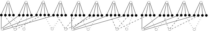 Figure 1
| 1 | 2 | 3 | 4 | 5 | 10 | 100 | 1000 | 10000 | 1000000 | |
|---|---|---|---|---|---|---|---|---|---|---|
| 1.2785 | 1.4631 | 1.6036 | 1.7179 | 1.8146 | 2.1569 | 3.6360 | 5.4214 | 7.3603 | 11.4673 | |
| 1.2167 | 1.3667 | 1.4834 | 1.5800 | 1.6637 | 1.9645 | 3.3428 | 5.0808 | 6.9967 | 11.0820 | |
| - | 1.0597 | 1.0046 | 1.0597 | 1.1336 | 1.4686 | 3.0780 | 4.9752 | 6.9901 | 11.1898 | |
| 1.6932 | 2.0987 | 2.3863 | 2.6095 | 2.7918 | 3.3979 | 5.6152 | 7.9088 | 10.2105 | 14.8156 |
Peer Reviews
No public reviews on file for this paper yet. If you reviewed it on a platform where reviews are public (OpenReview, ICLR, NeurIPS, ICML), you can paste yours below so the community can read it here.
Videos
No videos yet. Explain this paper in a talk, walkthrough, or lecture? Add one.
11institutetext: The Open University of Israel. 11email: [email protected], [email protected]
Approximating activation edge-cover and
facility location problems
Zeev Nutov
Eli Shalom
Abstract
What approximation ratio can we achieve for the Facility Location problem if whenever a client connects to a facility , the opening cost of is at most times the service cost of ? We show that this and many other problems are a particular case of the Activation Edge-Cover problem. Here we are given a multigraph , a set of terminals, and thresholds for each -edge . The goal is to find an assignment to the nodes minimizing , such that the edge set activated by covers . We obtain ratio for the problem, where is the root of the equation and is a problem parameter. This result is based on a simple generic algorithm for the problem of minimizing a sum of a decreasing and a sub-additive set functions, which is of independent interest. As an application, we get that the above variant of Facility Location admits ratio ; if for each facility all service costs are identical then we show a better ratio , where . For the Min-Power Edge-Cover problem we improve the ratio of [3] (achieved by iterative randomized rounding) to . For unit thresholds we improve the ratio of [3] to .
Keywords: generalized min-covering problem; activation edge-cover; facility location; minimum power; approximation algorithm
1 Introduction
Let be an undirected multigraph where each edge has an activating function from some range to . Given a non-negative assignment to the nodes, we say that a -edge is activated by if . Let denote the set of edges activated by . The value of an assignment is . In Activation Network Design problems the goal is to find an assignment of minimum value, such that the edge set activated by satisfies a prescribed property. We refer the reader to a paper of Panigrahi [16] and a recent survey [15] on activation problems, where also the following two assumptions are justified.
Monotonicity Assumption. For every , is monotone non-decreasing, namely, implies if and .
Polynomial Domain Assumption. Every has a polynomial size in set of “levels” and for every -edge .
Given a set of terminals we say that an edge set is an -cover or that ** covers ** if every has some edge in incident to it. In the Edge-Cover problem we seek an -cover of minimum value. The min-cost version of this problem can be solved in polynomial time [7], and it is one of the most fundamental problems in Combinatorial Optimization, cf. [19].
We consider the Activation Edge-Cover problem. Since we consider multigraphs, means that is a -edge, namely, that are the endnodes of ; means that is a -edge. Under the two assumptions above, the problem can be can be formulated without activating functions. For this, replace each edge by a set of at most -edges . Then for any the optimal assignment activating is given by ; here and everywhere a maximum or a minimum taken over an empty set is assumed to be zero. Consequently, the problem can be restated as follows.
Activation Edge-Cover
Input: A graph , a set of terminals , and thresholds for each -edge .
Output: An assignment of minimum value , such that the edge set activated by covers .
As we will explain later, Activation Edge-Cover problems are among the most fundamental problems in network design, that include NP-hard problems such as Set-Cover, Facility Location, covering problems that arise in wireless networks (node weighted/min-power/installation problems), and many other problems.
To state our main result we define assignments and , where if and for :
is the minimum threshold at of an edge in incident to .
, so is the minimum value of an edge in incident to .
The quantity is called the slope of the instance. We say that an Activation Edge-Cover instance is -bounded if the instance slope is at most , namely if for all ; moreover, we assume by default that is the instance slope. For each let be some minimum value edge covering . Then is an -cover of value at most . From this and the definition of we get
[TABLE]
In particular, . Using this, it is possible to design a greedy algorithm with ratio . We will show how to obtain a better ratio (the difference is quite significant when – see Table 1), as follows.
The Lambert -Function (a.k.a. ProductLog Function) is the inverse function of . It is known that for any , equals to the (unique) real root of the equation , and that . Our main result is:
Theorem 1.1
Activation Edge-Cover* admits ratio for -bounded instances. The problem also admits ratio , and ratio if is an independent set in , where is the maximum number of terminal neighbors of a node in .*
This result is based on a generic simple approximation algorithm for the problem of minimizing a sum of a decreasing and a sub-additive set functions, which is of independent interest; it is described in the next section. This result is inspired by the so called “Loss Contraction Algorithm” of Robins & Zelikovsky [18] for the Steiner Tree problem, and the analysis in [10] of this algorithm.
Let us say that is a steady node if the thresholds of the edges adjacent to are all equal the same number , which we call the weight of . Note that we may assume that all non-terminals are steady, by replacing each by new nodes; see the so called “Levels Reduction” in [15]. This implies that we may also assume that no two parallel edges are incident to the same non-terminal. Clearly, we may assume that is an independent set in . Let Bipartite Activation Edge-Cover be the restriction of Activation Edge-Cover to instances when also is an independent set, namely, when is bipartite with sides . Note that in this case is a simple graph and all non-terminals are steady.
We now mention some particular threshold types in Activation Edge-Cover problems, some known problems arising from these types, and some implications of Theorem 1.1 for these problems.
Weighted Set-Cover
This is a particular case of Bipartite Activation Edge-Cover when all nodes are steady and nodes in have weight [math]. Note that in this case is infinite, and we can only deduce from Theorem 1.1 the known ratio . Consider a modification of the problem, which we call -Bounded Weighted Set-Cover: when we pick a set , we need to pay for each element in covered by . Then the corresponding Activation Edge-Cover instance is -bounded.
Facility Location
Here we are given a bipartite graph with sides (clients) and (facilities), weights (opening costs) , and distances (service costs) . We need to choose with minimal, where is the minimal distance from to . This is equivalent to Bipartite Activation Edge-Cover. Note however that if for some constant we have for all with and , then the corresponding Bipartite Activation Edge-Cover instance is -bounded, and achieves a low constant ratio even for large values of .
Installation Edge-Cover
Suppose that the installation cost of a wireless network is proportional to the total height of the towers for mounting antennas. An edge is activated if the towers at and are tall enough to overcome obstructions and establish line of sight between the antennas. This is modeled as each pair has a height demand and constants , such that a -edge is activated by if the scaled heights sum to at least . In the Installation Edge-Cover problem, we need to assign heights to the antennas such that each terminal can communicate with some other node, while minimizing the total sum of the heights. The problem is Set-Cover hard even for thresholds and bipartite [16]. But in a practical scenario, the quotient of the maximum tower height over the minimum tower height is usually bounded by a constant; say, if possible tower heights are , then the slope is .
Min-Power Edge-Cover
This problem is a particular case of Activation Edge-Cover when for every edge ; note that in this case (in fact, the case is much more general). The motivation is to assign energy levels to the nodes of a wireless network while minimizing the total energy consumption, and enabling communication for every terminal. The Min-Power Edge-Cover problem is NP-hard even if , or if is an independent set in the input graph and unit thresholds [11]. The problem admits ratio by a trivial reduction to the min-cost case. This was improved to in [13], and then to in [3], where is also given ratio for the bipartite case and for unit thresholds.
From Theorem 1.1 and the discussion above we get:
Corollary 1
Min-Power Edge-Cover* admits ratio , and the -bounded versions of each one of the problems Weighted Set-Cover, Facility Location, and Installation Edge-Cover, admits ratio .*
Let us illustrate this result on the Facility Location problem. One might expect a constant ratio for any , but our ratio is surprisingly low. Even if (service costs are at least of opening costs) then we get a small ratio . Even for we still get a reasonable ratio . All previous results for the problem are usually summarized by just two observations: the problem is Set-Cover hard (so has a logarithmic approximation threshold by [17, 8]), and that it admits a matching logarithmic ratio [5]; see surveys on Facility Location problems by Vygen [22] and Shmoys [20]. Due to this, all work focused on the more tractable Metric Facility Location problem. Our Theorem 1.1 implies that many practical non-metric Facility Location instances admit a reasonable small constant ratio.
For the case of “locally uniform” thresholds – when for each non-terminal (facility) all thresholds (service costs) are identical, we show a better ratio, see also Table 1. In what follows, let denote the -th harmonic number.
Theorem 1.2
Bipartite* Activation Edge-Cover with locally uniform thresholds admits ratio , where .*
We do not have a convenient formula for , but in Section 4 we observe that the maximum is attained for the smallest integer such that . We will show that for all , and that , so both and are close to for large values of , although the convergence is very slow; see also Table 1.
We will also show that . Note that our Theorem 1.1 ratio for significantly improves the previous best ratio of [3] for Min-Power Edge-Cover on general graphs achieved by iterative randomized rounding; we do not match the ratio of [3] for the bipartite case, but note that the case is much more general than the min-power case considered in [3].
Theorem 1.2 has some applications for the Set-Cover problem. Given a Set-Cover instance represented by a bipartite graph, obtain a Bipartite Activation Edge-Cover instance by assigning unit weights to sets (non-terminals) and a threshold to every terminal (element). These threshold are locally uniform and the obtained instance has slope . For this instance the Theorem 1.2 algorithm coincides with the standard greedy algorithm, and computes a Set-Cover solution of size , where is the optimal size of a Set-Cover solution. Substituting and dividing by we get that for any the greedy algorithm for Set-Cover achieves ratio . We note that Slavik [21] proved that the greedy algorithm for Set-Cover achieves ratio , while our ratio for locally uniform thresholds is ; we will discuss the relation between these two results in the full version.
In addition, we consider unit thresholds, and using some ideas from [3] improve the previous best ratio of [3] as follows.
Theorem 1.3
Activation Edge-Cover* with unit thresholds admits ratio .*
We note that our main contribution is not technical, although some proofs are non-trivial (the reader may observe that proofs of many seemingly complicated results were substantially simplified with years, by additional effort). Our main contribution is giving a unified algorithm for a large class of problems that we identify – -Bounded Activation Edge-Cover problems, either substantially improving known ratios, or showing that many seemingly Set-Cover hard problems may be tractable in practice. Let us also point out that our main result is more general than the applications listed in Corollary 1. The generalization to -bounded Activation Edge-Cover problems is different from earlier results; besides finding a unifying algorithmic idea generalizing and improving previous results, we are also able to find tractable special cases in a new direction.
The rest of this paper is organized as follows. In Section 2 we define the Generalized Min-Covering problem and analyze a greedy algorithm for it, see Theorem 2.1. In Section 3 we use Theorem 2.1 to prove Theorem 1.1. Theorems 1.2 and 1.3 are proved using a modified method in Sections 4 and 5, respectively.
2 The Generalized Min-Covering problem
A set function is increasing if whenever ; is decreasing if is increasing, and is sub-additive if for any subsets of the ground-set. Let us consider the following algorithmic problem:
Generalized Min-Covering
Input: Non-negative set functions on subsets of a ground-set such that is decreasing, is sub-additive, and .
Output: such that is minimal.
The “ordinary” Min-Covering problem is ; it is a particular case of the Generalized Min-Covering problem when we seek to minimize for a large enough constant . Under certain assumptions, the Min-Covering problem admits ratio [12]. Various generic covering problems are considered in the literature, among them the Submodular Covering problem [23], and several other types, cf. [4]. The variant we consider is inspired by the algorithms of Robins & Zelikovsky [18] for the Steiner Tree problem, and the analysis in [10] of this algorithm; but, to the best of our knowledge, the explicit formulation of the Generalized Min-Covering problem given here is new. Interestingly, our ratio for Min-Power Edge-Cover is the same as that of [18] for Steiner Tree in quasi-bipartite graphs.
We call the potential and the payment. The idea behind this interpretation and the subsequent greedy algorithm is as follows. Given an optimization problem, the potential is the value of some “simple” augmenting feasible solution for . We start with an empty set solution, and iteratively try to decrease the potential by adding a set of minimum “density” – the price paid for a unit of the potential. The algorithm terminates when the price , since then we gain nothing from adding to . The ratio of such an algorithm is bounded by (assuming that during each iteration a minimum density set can be found in polynomial time). So essentially the greedy algorithm converts ratio into ratio . However, sometimes a tricky definition of the potential and the payment functions may lead to a smaller ratio.
Let be the optimal solution value of a problem instance at hand. Fix an optimal solution . Let , , so . The quantity is called the density of (w.r.t. ); this is the price paid by for a unit of potential. The Greedy Algorithm (a.k.a. Relative Greedy Heuristic) for the problem starts with and while repeatedly adds to a non-empty augmenting set that satisfies the following condition, while such exists:
Density Condition: .
Note that since is decreasing ; hence if , then and there exists an augmenting set that satisfies the condition , e.g., . Thus if is a minimum density set and , then satisfies the Density Condition; otherwise, no such exists.
Theorem 2.1
The Greedy Algorithm achieves approximation ratio
[TABLE]
Proof
Let be the number of iterations. Let and for let be the intermediate solution at the end of iteration and . Let , . Then:
[TABLE]
Since is decreasing
[TABLE]
This is the lower Darboux sum of the function \displaystyle f(\nu)=\left\{\begin{array}[]{ll}1&\mbox{ if }\nu\leq\tau^{*}+\nu^{*}\\ \frac{\tau^{*}}{\nu-\nu^{*}}&\mbox{ if }\nu>\tau^{*}+\nu^{*}\end{array}\right. in the interval w.r.t. the partition . We claim that . For this, note that , thus since is decreasing . Consequently, is bounded by
[TABLE]
Let be the set computed by the algorithm. Since is sub-additive
[TABLE]
Thus the approximation ratio is bounded by . ∎
3 Algorithm for general thresholds (Theorem 1.1)
Given an instance of Activation Edge-Cover the corresponding Generalized Min-Covering instance is defined as follows. We put at each node a large set of “assignment units”, and let be the union of these sets of “assignment units”. Note that to every naturally corresponds the assignment where is the number of units in put at . It would be more convenient to define and in terms of assignments, by considering instead of a set the corresponding assignment .
To define and , let us recall the assignments and from the Introduction. We have if and for :
is the minimum threshold at of an edge in incident to .
, so is the minimum value of an edge in incident to .
We let and . Note that for any ; in particular, . For an assignment that “augments” let denote the set of terminals covered by . A natural definition of the potential and the payment functions would be and but this will enable to prove only ratio . We show a better ratio by adding to the potential in advance the “fixed” part . We define
[TABLE]
It is easy to see that is decreasing, is sub-additive, and .
The next lemma shows that the obtained Generalized Min-Covering instance is equivalent to the original Activation Edge-Cover instance.
Lemma 1
If is a feasible solution for Activation Edge-Cover then . If is a feasible solution for Generalized Min-Covering then one can construct in polynomial time a feasible solution for Activation Edge-Cover of value at most . In particular, both problems have the same optimal value, and Generalized Min-Covering has an optimal solution such that and thus .
Proof
If is a feasible Activation Edge-Cover solution then and thus . Consequently, .
Let now be a Generalized Min-Covering solution. The assignment has value and activates the edge set that covers . To cover , pick for every an edge with minimum. Let be an assignment defined by if and otherwise. The set of picked edges can be activated by an assignment that has value . The assignment activates both edge sets and has value , as required. ∎
For the obtained Generalized Min-Covering instance, let us fix an optimal solution as in Lemma 1, so and . Denote , and note that . To apply Theorem 2.1 we need several bounds given in the next lemma.
Lemma 2
, , and .
Proof
Note that
[TABLE]
In particular, , and this implies the first bound of the lemma
[TABLE]
The second bound of the lemma holds since .
The last bound of the lemma is equivalent to the bound . Let be an inclusion minimal edge cover of activated by . Then is a collection of node disjoint rooted stars with leaves in . Let . By the definition of , , thus . Consequently, . ∎
We will show later that the Greedy Algorithm can be implemented in polynomial time; now we focus on showing that it achieves the approximation ratios stated in Theorem 1.1. Substituting Lemma 2 second bound in Theorem 2.1 second bound and denoting , we get that and that the ratio is bounded by
[TABLE]
Consequently, the the ratio is bounded by . We now derive a formula for the maximum. We have (this can be shown using L’Hospital’s Rule), and . Also:
[TABLE]
Hence if and only if , namely, . For the analysis, we substitute , and get the equation , where . Since the function is strictly increasing and the function is strictly decreasing, this equation has at most one root; we claim that this root exists and is in the interval . To see this consider the function , and note that is continuous and that while for small enough.
From this we get that the ratio is bounded by , where is the root of the equation .
Substituting Lemma 2 third bound in Theorem 2.1 first bound and observing that we get that the ratio is bounded by . In the case when is an independent set in , it is easy to see that Lemma 2 third bound improves to , and we get ratio in this case.
Finally, we show that the Greedy Algorithm algorithm can be implemented in polynomial time. As was mentioned in Section 2 before Theorem 2.1, we just need to perform in polynomial time the following two operations for any assignment : to check the condition , and to find an augmenting assignment of minimum density.
It is is easy to see that assignments and can be computed in polynomial time, and thus the potential can be computed in polynomial time, for any . Let be an optimal solution as in Lemma 1, and denote and . Then the condition is equivalent to and thus can be checked in polynomial time.
Now we show how to find an augmenting assignment of minimum density. Note that the density of an assignment w.r.t. is
[TABLE]
Lemma 3
There exists a polynomial time algorithm that given an instance of Activation Edge-Cover and an assignment finds an assignment of minimum density.
Proof
A star is a rooted tree with at least one edge such that only its root may have degree . We say that a star is a proper star if all the leaves of are terminals. We denote the terminals in by .
Since are given assignments, we may simplify the notation by assuming that is our set of terminals, and that is our given assignment. Then the density of is just . Let be an assignment of minimum density, and let be an inclusion minimal -cover. Then decomposes into a collection of node disjoint proper stars that collectively cover . For let be the optimal assignment such that activates . Since the stars in are node disjoint
[TABLE]
By an averaging argument, holds for some , and since is a minimum density assignment, so is , and holds. Consequently, it is sufficient to show how to find in polynomial time an assignment such that activates a proper star and is minimal.
We may assume that we know the root and the value of an optimal density pair ; there are at most choices and we can try all and return the best outcome. Let . For let be the minimal non-negative number for which there is a -edge with and . Then our problem is equivalent to finding with minimum. This problem can be solved in polynomial time, by starting with and while there is with , adding to with minimum. ∎
The proof of Theorem 1.1 is complete.
4 Locally uniform thresholds (Theorem 1.2)
Here we consider the Bipartite Activation Edge-Cover problem with locally uniform thresholds. This means that each non-terminal has weight and all edges incident to have the same threshold ; in the -bounded version . We consider a natural greedy algorithm that repeatedly picks a star that minimizes the average price paid for each terminal (the quotient of the optimal activation value of over ), and then removes . Each time we choose a star we distribute its activation value uniformly among its terminals, paying in the computed solution the average price for each terminal of .
We now apply a standard “set-cover” analysis, cf. [24]. In some optimal solution fix an inclusion maximal star with center and terminals covered by the algorithm in the order , where is covered first and last; we bound the algorithm payment for covering . Note that . Denote and let be the threshold of the terminals in . Let be the substar of with leaves . At the start of the iteration in which the algorithm covers , the terminals of are uncovered. Thus the algorithm pays for covering at most the average price paid by , namely . Over all iterations, the algorithm pays for covering at most , while the optimum pays . Thus the quotient between them is bounded by
[TABLE]
Since any optimal solution decomposes into node disjoint stars, the last term bounds the approximation ratio, concluding the proof of Theorem 1.2. We make some observations about this bound. Let . We have
[TABLE]
Thus if and only if . Hence if is the smallest integer such that then . We do not have a more convenient formula of for arbitrary , but we can bound it using the inequality . Then we have:
[TABLE]
Using fundamental calculus one can see that the maximum is attained when , and substituting this in we get that where is the solution to the equation . We have . Thus the ratio is bounded by , a bound that we got before in Theorem 1.1.
If then , since and . We have , so for we get ratio . The ratio is tight for unit thresholds, as shows the example in Fig. 1. The instance has terminals (in black), and two sets of covering nodes: the upper nodes that form an optimal cover, and the bottom nodes. The bottom nodes have nodes of degree , of degree , and of degree . The algorithm may start taking all bottom nodes, and only then add the upper ones, thus creating a solution of value , instead of the optimum .
5 Unit thresholds (Theorem 1.3)
Here we consider the case of unit thresholds when for every -edge . By a reduction from [3], we may assume that the instance is bipartite. Specifically, for any optimal assignment we have for all , hence we can consider the residual instance obtained by removing the terminals covered by edges with both ends in ; in the new obtained instance is an independent set, and recall that we may assume that is an independent set.
One can observe that in the obtained bipartite instance, is an optimal solution if and only if for all , for all , and the set covers , meaning that is the set of neighbors of . Namely, our problem is equivalent to . On the other hand the problem is essentially the (unweighted) Set-Cover problem, and is a feasible solution to this Set-Cover instance if and only if is the characteristic set of a feasible assignment for the Activation Edge-Cover instance. Note that both problems are equivalent w.r.t. their optimal solutions but may differ w.r.t. approximation ratios, since if is an optimal solution to the Set-Cover instance then may be much smaller than .
Recall that a standard greedy algorithm for Set-Cover repeatedly picks the center of a largest star and removes the star from the graph. This algorithm has ratio for -Set-Cover, where is the maximum degree of a non-terminal (the maximum size of a set). However, the same algorithm achieves a much smaller ratio for Activation Edge-Cover with unit thresholds; the ratio was established in [3], and it also follows from the case in Theorem 1.2. In what follows we denote by the best known ratio for -Set-Cover. We have ( is the Edge-Cover problem) and [6]. The current best ratios for are due to [9] (see also [14, 1]). We summarize the current values of for in the following table.
We now show how these ratios for -Set-Cover can be used to approximate the Activation Edge-Cover problem with unit costs. We start by describing a simple algorithm with ratio , that uses only the case.
We claim that the above algorithm achieves approximation ratio for Activation Edge-Cover (a similar analysis implies ratio for Set-Cover). In some optimal solution fix a star with terminals covered in the order , where is covered first and last; we bound the algorithm payment to cover these terminals. Let be the substar of with leaves . At the start of the iteration when is covered, the terminals of are uncovered. Thus the algorithm pays for covering at most the density of , namely, . Over all iterations, the algorithm pays for covering at most , while the optimum pays . If then the algorithm pays at most the amount of the optimum. We claim that if then in fact the payment is at most . If then the payment is at most (we pay if the star “survives” all the iterations before the last). For , the pay for the last terminals is either: for each of for and for (a total of ), or for and for (a total of ). The maximum is . Consequently, the ratio is bounded by
[TABLE]
By fundamental computations we have . Thus is increasing iff . Since and , we get that , so we have ratio .
We now show ratio . As in the greedy algorithm for Set-Cover, we repeatedly remove an inclusion maximal set of disjoint stars with maximum number of leaves and pick the set of roots of these stars. The difference is that each time stars with more than leaves are exhausted, we compute an -approximate solution for the remaining -Set-Cover instance; we let . This gives many Set-Cover solutions, each is a union of the centers of stars picked and ; we choose the smallest one, and together with this gives a feasible Activation Edge-Cover solution. Formally, the algorithm is:
Since we claim ratio , at iterations when step 3 can be skipped, since then we can apply a standard “local ratio” analysis [2]. Indeed, when a star with terminals is removed, the partial solution value increases by while the optimum decreases by at least . Hence for it is a local ratio step. Consequently, we may assume that , provided that we do not claim ratio better than .
Let . Let be the optimal value to the initial Set-Cover instance. At iteration the algorithm computes a solution of value at most . Thus we get ratio if holds for some . Otherwise,
[TABLE]
Denote . Note that , since in this sum the number of stars with leaves is summed exactly times, . The first inequality, and the inequality obtained as the sum of the other six inequalities gives the following two inequalities:
[TABLE]
Dividing both inequalities by and denoting gives:
[TABLE]
Since and this is equivalent to:
[TABLE]
We obtain a contradiction if is the solution of the equation , namely
[TABLE]
This concludes the proof of Theorem 1.3.
The reference list from the paper itself. Each links out to its DOI / PubMed record.
- 1[1] S. Athanassopoulos, I. Caragiannis, and C. Kaklamanis. Analysis of approximation algorithms for k 𝑘 k -set cover using factor-revealing linear programs. Theory Comput. Syst. , 45(3):555–576, 2009.
- 2[2] R. Bar-Yehuda. One for the price of two: A unified approach for approximating covering problems. Algorithmica , 27(2):131–144, 2000.
- 3[3] G. Calinescu, G. Kortsarz, and Z. Nutov. Improved approximation algorithms for minimum power covering problems. In WAOA , pages 134–148, 2018.
- 4[4] K. Chandrasekaran, R. M. Karp, E. Moreno-Centeno, and S. Vempala. Algorithms for implicit hitting set problems. In SODA , pages 614–629, 2011.
- 5[5] V. Chvatal. Greedy heuristic for the set-covering problem. Mathematics of Operations Research , 4(3):233–235, 1979.
- 6[6] R.-c. Duh and M. Fürer. Approximation of k 𝑘 k -set cover by semi-local optimization. In STOC , pages 256–264, 1997.
- 7[7] J. Edmonds. Paths, trees, and flowers. Canadian Journal of Mathematics , 17:449–467, 1965.
- 8[8] U. Feige. A threshold of ln n 𝑛 \ln n for approximating set cover. J. of the ACM , 45(4):634–652, 1998.