The content correlation of multiple streaming edges
Michel de Rougemont, Guillaume Vimont

TL;DR
This paper introduces an efficient online method to detect and analyze content correlations between multiple streaming graph edges, enabling real-time clustering and search applications like Twitter stream analysis.
Contribution
It extends clustering and correlation detection to dynamic, multi-stream graphs without full storage, providing guarantees for power-law distributed random graphs.
Findings
Effective online approximation of content correlation in streaming graphs
Successful application to Twitter data streams
Enables correlation-based search and explanation mechanisms
Abstract
We study how to detect clusters in a graph defined by a stream of edges, without storing the entire graph. We extend the approach to dynamic graphs defined by the most recent edges of the stream and to several streams. The {\em content correlation }of two streams is the Jaccard similarity of their clusters in the windows before time . We propose a simple and efficient method to approximate this correlation online and show that for dynamic random graphs which follow a power law degree distribution, we can guarantee a good approximation. As an application, we follow Twitter streams and compute their content correlations online. We then propose a {\em search by correlation} where answers to sets of keywords are entirely based on the small correlations of the streams. Answers are ordered by the correlations, and explanations can be traced with the stored clusters.
Click any figure to enlarge with its caption.
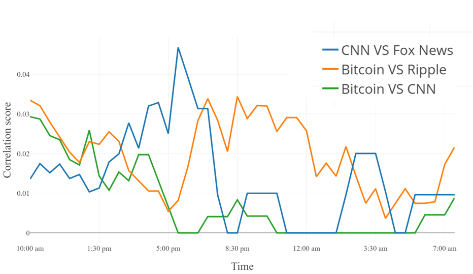 Figure 1
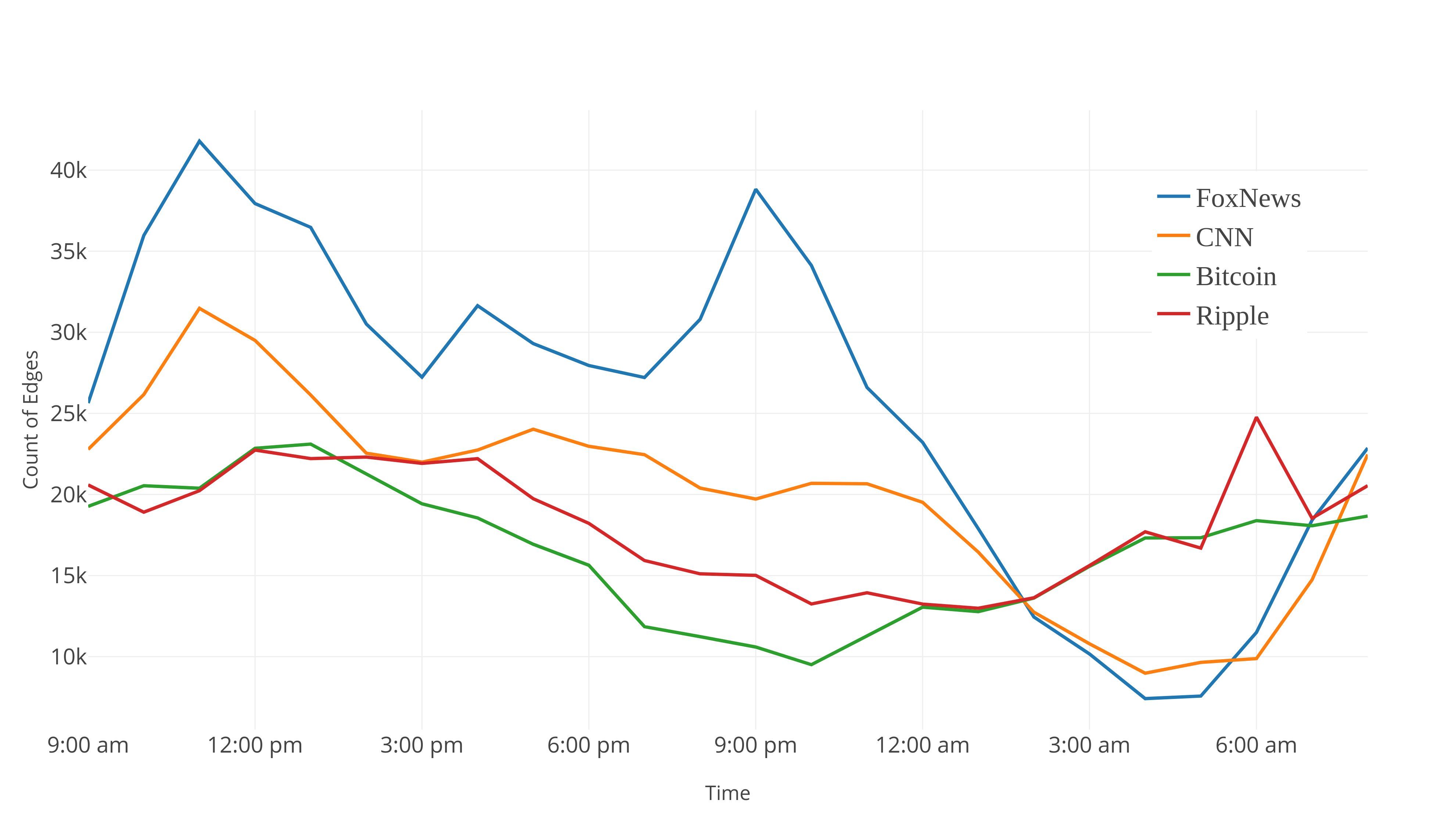 Figure 2
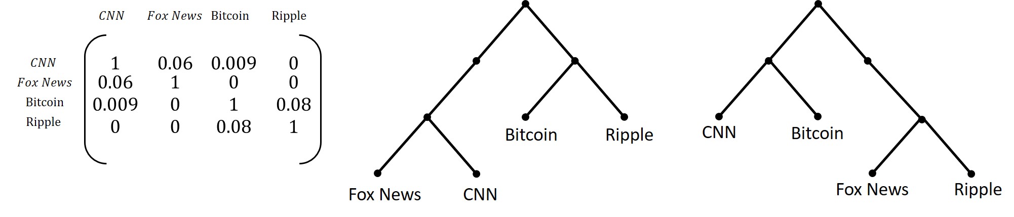 Figure 3
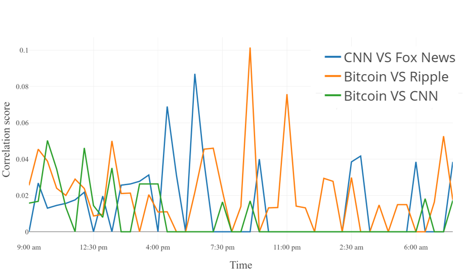 Figure 4
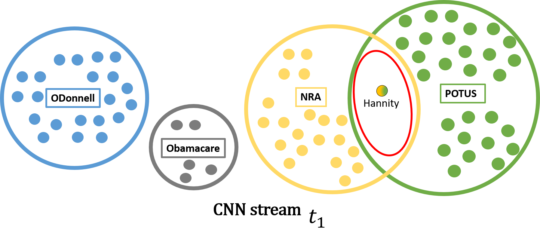 Figure 5
| Input: CNN | Input: CNN POTUS | Input: CNN POTUS NRA | |||||||||
| Ranking | t =12 | t = 24 | Ranking | t = 12 | t = 24 | Ranking | t = 12 | ||||
| 1 | #ODonnell | #POTUS | 1 | #MondayMotivaton | #Tucker | 1 | #Hannity | ||||
| 2 | #NRA | #NRA | 2 | #Hannity | #2A | 2 | #2A | ||||
| 3 | #POTUS | #ODonnell | 3 | #NRA | #NRA | 3 | #1A | ||||
| 4 | #Obamacare | #Tucker | 4 | #1A | #1A | 4 | #Clinton | ||||
| 5 | #MondayMotivaton | #2A | 5 | #Tucker | #Hannity | 5 | #ClintonFoundation | ||||
Peer Reviews
No public reviews on file for this paper yet. If you reviewed it on a platform where reviews are public (OpenReview, ICLR, NeurIPS, ICML), you can paste yours below so the community can read it here.
Videos
No videos yet. Explain this paper in a talk, walkthrough, or lecture? Add one.
Taxonomy
TopicsComplex Network Analysis Techniques · Data Management and Algorithms · Peer-to-Peer Network Technologies
The content correlation of multiple streaming edges
Michel de Rougemont 1
Guillaume Vimont1
(1 University Paris II, CNRS-IRIF
)
Abstract
We study how to detect clusters in a graph defined by a stream of edges, without storing the entire graph. We extend the approach to dynamic graphs defined by the most recent edges of the stream and to several streams. The *content correlation *of two streams is the Jaccard similarity of their clusters in the windows before time . We propose a simple and efficient method to approximate this correlation online and show that for dynamic random graphs which follow a power law degree distribution, we can guarantee a good approximation. As an application, we follow Twitter streams and compute their content correlations online. We then propose a search by correlation where answers to sets of keywords are entirely based on the small correlations of the streams. Answers are ordered by the correlations, and explanations can be traced with the stored clusters.
Keywords: Streaming algorithms, Dynamic graphs, Clustering, Approximation
1 Introduction
Consider a stream of edges of a graph which follows a power law degree distribution. Sliding windows define dynamic graphs and we select each edge with a uniform probability in each window. There are several techniques which generalize the original Reservoir sampling [12] for a fixed window, to dynamic windows. At any given time , we have a Reservoir which keeps edges among the possible edges which have been read (), and each edge has the same probability to be chosen in the Reservoir. If the cluster and the Reservoir size are large enough, a large connected component will appear in the Reservoir. The random edges of are taken with the same probability , i.e. follow the Erdös-Renyi model and the giant component in occurs if , the classical phase transition probability. In the dynamic case, we will observe changes in the communities as new communities appear and old communities disappear. At discrete times we store only the large connected components of the Reservoirs.
We study the correlation between multiple streams of graph edges and define the content correlation of two streams of edges, based on the Jaccard similarity of their clusters and extend it to on the dynamic graphs . We provide an analysis of dynamic random graphs which follow a power law degree distribution, based on the Configuration Model [10]. We give sufficient conditions to detect clusters depending on their size, the Reservoir size and the length of the observation. We then approximate the content correlation with an online algorithm, i.e. estimate the correlation at discrete times .
Streams of graph edges are ubiquitous, in particular in social networks where the graphs have a degree distribution close to a power law, a small diameter and clusters (communities) which evolve in time. Twitter streams are defined by some tags and generate a stream of edges of large dynamic graphs. We estimate the correlations between multiple streams and obtain a correlation matrix , from which we build a phylogeny tree. We then introduce a Search by correlation: given some tags, we find the most correlated tags which depend on the history of the clusters and on the phylogeny tree. Our main results are:
- •
We propose an Algorithm which detects large static clusters in a graph which follows a power law degree distribution, with high probability, using only a few edge samples (theorem 1) and its extension to dynamic graphs (theorem 2),
- •
We present an online algorithm for . For two dynamic graphs with clusters and whose Jaccard similarity is , the correlation is close to (theorem 3).
We estimated the content correlations of Twitter streams (approximately edges) over h online and built the closest phylogeny tree. The Search by correlation illustrates the technique which uses the correlations, a phylogeny tree and the stored clusters. In the second section, we define the framework of dynamic graphs defined by a stream of edges and introduce the notion of content correlation of two streams. In the third section, we set a model of random dynamic graphs where we can guarantee the approximation of the correlation. In the fourth section, we present our analysis of multiple Twitter channels and their correlations. In the fifth section, we introduce the Search by correlation, using a phylogeny tree built from the correlation matrix of the streams.
2 Dynamic graphs in a window of streaming edges
Let be a stream of edges where each . It defines a graph where is the set of nodes and is the set of edges: we allow self-loops and multi edges and assume that the graph is symmetric. In the *window model * we isolate the most recent edges at some discrete . There are two models of sliding windows: the most recent edges or the most recent edges in some fixed time interval . If the rate (the number of edges per time unit) of the stream is fixed, both models coincide. It is not the case in practice, as the rate fluctuates within a factor at any given time. We take the second model, i.e. keep the length of the window , hence and each for and determines a window of length and a graph defined by the edges in the window or time interval . The number of edges in a window may increase or decrease and reflects the increasing or decreasing rates of a stream. Consecutive windows overlap within a factor , about in the experiments. In practice, mins and mins. The graphs and share many edges: old edges of are removed and new edges are added to . Social graphs have a specific structure, a specific degree distribution (power law), a small diameter and some dense clusters. The dynamic random graphs introduced in the next section satisfy these conditions.
There are several definitions of a cluster or community or dense subgraph. We consider a cluster of domain as a maximal dense subgraph which depends on a parameter . Let and let be the multiset of internal edges i.e. edges where . A -cluster is maximal subset such that . There are several other possible definitions of clusters which capture the high internal global density, and there are many algorithms to detect such clusters in a static graph. We are mainly interested in the approximate detection of clusters in the dynamic case, without storing the whole graph.
2.1 Detecting clusters in a stream of edges
If the entire graph is known, there are several classical techniques to approximate communities. For , the problem is known as Maxclique, which is NP-hard. In our framework, we do not store the entire graph but only a few edges, and will only approximate the communities. We take a uniform sampling of the edges111Notice that such a uniform sampling on the edges is equivalent to a sampling of the nodes proportionally to their degrees. for each window of the stream which defines , and keep samples in Reservoirs for a fixed size . There are several techniques to build such dynamic Reservoirs [4].
The sampling method we propose is not new, it is one of the sampling methods in [3]. Its analysis for dynamic graphs which follow a power law degree distribution is one of the central points of this paper. If a cluster is large, there will be a large connected component in the Reservoir as a witness. We ignore all the small connected components of the Reservoir and only store in a database the large ones. In a typical experiment whereas we read edges in a window. We ignore all the components of size less than , a threshold value. For a graph , there could be several large clusters or there could be none. For a stream , we write for the -th cluster of the stream at time .
2.2 Correlations
The classical correlation, also called the Pearson correlation of two random variables of mean and standard deviation is . How could it be extended to graphs? One could choose some statistics on the graphs and take the correlations between the statistical parameters. Social graphs have however very similar statistics and yet the core of the information seems to hide in the structure of their clusters. Given two graphs and , a first approach to their content correlation would be to consider the Jaccard similarity222The Jaccard similarity or Index between two sets and is . The Jaccard distance is . on the domains of the two graphs. It has several drawbacks: it is independent of the structures of the graphs, it is very sensitive to noise, nodes connected with one or few edges and it is not well adapted when the sizes are very different. It also requires to store the entire graphs.
We propose instead the following approach: we first estimate the dense components (clusters or communities) using the uniform sampling on the edges in the sliding windows and apply the Jaccard similarity only to these large dense components. It exploits the structure of the graphs, is insensitive to noise and adapts well when the graphs have different sizes. Let be the set of clusters of the graph , for or . The correlation of two graphs . This definition is for the first window or for two static graphs. For two dynamic streams and which share a time scale, we generalize to . The correlation of two graph streams and is . We can refine the correlation and define an amortized correlation , to give more importance to the recent components. In the next section, we give an algorithmic solution for graphs presented as streams of edges which scales when we consider dynamic graphs.
2.3 What is stored over time
At some discrete times , we store the large connected components of the Reservoirs . There could be none. We use a NoSQL database, with (Key, Values) tables where the key is always a tag (@x or #y) and the Values store the clusters nodes. Notice that a stream is identified by a tag (or a set of tags) and a cluster is also identified by a tag, its node of highest degree.
- •
Stream(tag, list(cluster, timestamp)) is the table which provides the most recent clusters of a stream,
- •
Cluster(tag, list(stream, timestamp, list(high-degree nodes), list(nodes,degree)))) is the table which provides the list of high-degree nodes and the list of nodes with their degree, in a given cluster,
- •
Nodes(tag, list(stream, cluster, timestamp)) is the table which provides for each node the list of streams, clusters and timestamps where the node appears,
- •
Correlation((tag1,tag2), list(value,timestamp)) is the table which provides for each pair of streams (tag1,tag2) the different correlation values .
2.4 Other approaches
There are many other approaches to detect clusters in streams of graphs edges. The dynamic graphs algorithms community studies the compromise between update and query time in the worst case. The graph streaming approach [8] emphasizes the space complexity in the worst case and in particular for the window model. The network sampling approach such as [3] does consider the uniform sampling on the edges but there is no analysis for the detection of clusters in dynamic graphs. The detection of a planted clique is a classical problem [6], hard when the clique size is for example in the worst case. The *graph mining community * [2, 1, 13] studies the detection of clusters when the graphs are entirely known.
In our approach, we only consider classes of graphs which follow a power law degree distribution, and study approximate algorithms for the detection of dynamic -cliques in the window model using only small Reservoirs.
3 Deciding properties and correlations in dynamic random models
We define a model of dynamic random graphs which may or may not have clusters and follow a degree distribution using the Configuration Model. Temporal Logic is a framework to decide temporal properties of the dynamic graphs . Let be a graph property such as Connectivity, or the existence of a -cluster of size at least . A typical temporal property is stating that there exists a such that or stating that for all , . In this section, we show that the algorithmic approach guarantees a good approximation of the correlation with high probability.
3.1 Dynamic Random graphs
The classical Erdös-Renyi model [5], generates random graphs with nodes and edges are taken independently with probability where . The degree distribution is close to a gaussian centered on . Most of the social graphs have a degree distribution close to a power law, such as a Zipfian distribution distribution where , where is the degrre of a node. In this case, the maximum degree is . The Configuration Model for and a graph with nodes enumerates each node with half-edges (stubs) and takes a symmetric random matching between two stubs, for example with a uniform permutation such that . All the possible graphs are obtained with a distribution close to the uniform distribution.
A classical study is to find sufficient conditions so that a random graph has a giant component, i.e. of size for a graph of size . In the Erdös-Renyi model , it requires that , and in the Configuration Model it requires that as proved in [9], which is realized for the Zipfian distribution. There is a phase transition for both models. There are several possible extensions to dynamic random graphs. In our model, the Dynamics is exogenous and at any time chooses between the Uniform and the Concentrated Dynamics.
3.1.1 Uniform Dynamics
we generalize the Configuration Model in a dynamic setting. Remove random edges, uniformly on the set of edges of , freeing stubs. Generate a new uniform matching on these hubs to obtain . The distribution of random graphs stays uniform.
3.1.2 Concentrated Dynamics
a typical graph generated by the Uniform Dynamics is not likely to have a large cluster. The -concentrated Dynamics fixes some a subset among the nodes of high degree. Remove edges, uniformly on the set of edges of , freeing stubs, as before. A stub is in if its origin or extremity is in . With probability , match the stubs in uniformly in . With probability , match the stubs in uniformly in . This dynamics will concentrate edges in and will create a -cluster after a few iterations with high probability, assuming the degree distribution is a power law. The distribution of graphs with a -cluster stays also uniform.
3.1.3 General Dynamics
a general Dynamics is a function which chooses at any given time, one of the two strategies: either a Uniform Dynamics or some -concentrated Dynamics for a fixed . An example is the Step Dynamics: apply the Uniform Dynamics first, then switch to the -dynamics for a time period , and switch back to the Uniform Dynamics. In our setting, the Dynamics depends on some external information, which we try to approximately recover. Notice that during the Uniform Dynamics phase, there are no large components and we store nothing. For the step phase, we store some components which will approximate . More complex strategies could involve several clusters and which may or may not intersect.
3.2 Deciding a static property: there is a large -cluster
Let be the Reservoir of size after we read edges . In this simple case, we first fill the Reservoir with . For , we decide to keep with probability and if we keep , we remove one of the edges (with probability ) to make room for . Each edge has then probability to be in the Reservoir, i.e. uniform.
The probabilistic space is determined by the choices taken at every step by the Reservoir sampling. Consider a clique in the graph: its image in the Reservoir is the set of internal edges in the Reservoir, where . Each edge of the clique is selected with constant probability , so we are in the case of the Erdös-Renyi model where and . We know that the phase transition occurs at , i.e. there is a giant component if and the graph is connected if .
In the case of a -clusters associated with the -concentrated Dynamics, the phase transition occurs at . Let be the set of nodes of the giant component whose nodes are in . As it is customary for approximate algorithms, we write to say that the Condition is true with high probability.
Lemma 1
For large enough, there exists and such that if in the concentrated Dynamics, then .
**Proof : ** If is almost a clique, i.e. a -cluster, then the phase transition occurs at . Hence if , there is a giant component of size larger than a constant times , say with high probability . As the probability of the edges is , it occurs if . Hence for large enough, there exists such that .
In order to decide the graph property : there is a large -cluster, consider this simple algorithm.
Static Cluster detection Algorithm 1: let be the largest connected component of the Reservoir . If then Accept, else Reject.
Theorem 1
If for the concentrated Dynamics, then:
**
and for the uniform Dynamics:
.
**Proof : ** If for the concentrated Dynamics, Lemma 1 states that with high probability, hence as , the condition is true with high probability hence . For the Uniform Dynamics (), [9] shows that the largest connected component has size . Hence .
Notice that , as the average degree in a power law is . If and , it satisfies the condition and it can be realized with the nodes of high degree.
3.3 Deciding a dynamic property:
Let be the previous property: is there a -cluster? How do we decide ? Consider the step strategy of length . When we switch strategy at time there is a delay until is a -cluster and symmetrically the same delay when we switch again at time . The probabilistic space is now much larger.
Dynamic Cluster detection Algorithm 2: let be the largest connected component of a dynamic Reservoir at time . If there is an such that , then Accept, else Reject.
We can still distinguish between the Uniform and the -concentrated Dynamics, if is large enough. Let be the number of edges in the window at time . Let be a graph defined by a stream of edges following a power law .
Theorem 2
For the step Dynamics of length and , if , then For the Uniform Dynamics .
**Proof : ** For each window, we can apply theorem 1 and there are independent windows. If for the concentrated Dynamics, the error probability is smaller than the error made for independent windows, which is . Hence . For the Uniform Dynamics (equivalent to ), the algorithm needs to be correct at each step. Hence .
The probability to accept for the concentrated Dynamics is amplified whereas the probability to reject for the Uniform Dynamics decreases. One single error generates a global error. Clearly, we could also estimate , for step strategies with similar techniques.
3.4 Correlation between two streams
Suppose we have two streams and which share the same clock. Suppose that is a step strategy on a cluster and is a step strategy on a cluster . Let . How good is the estimation of their correlation? Let be the set of large clusters at time of the graph , for or . Consider the following online algorithm to compute :
Online Algorithm 3 for . At time , compute the increase in size of for from , and the increase in size of . Suppose where and . Then: .
A simple computation shows that , i.e. the correct definition. The are computed by standard operations on sets.
Theorem 3
Let and be two step strategies before time on two clusters such that for . Then .
**Proof : ** After the first observed step, for example on , Lemma 1 indicates that is already some approximation of . After independent trials, will be a good approximation of . Similarly for and therefore will approximate .
4 Twitter streams
Given a set of tags such as #CNN or #Bitcoin, Twitter provides a stream of tweets represented as Json trees whose content contains at least one of these tags. The Twitter Graph of the stream, is the graph with multiple edges where is the set of tags or seen and for each tweet sent by which contains tags , we construct the edges and in . The URL’s which appear in the tweet can also be considered as nodes but we ignore them for simplicity. A stream of tweets is then transformed into a stream of edges .
We simultaneously captured twitter streams333Using a program available on https://github.com/twitterUP2/stream which takes some tags, a Reservoir size , a window size , a step and saves the large connected components of the Reservoirs . on the tags #CNN, #FoxNews, #Bitcoin, and #Xrp (Ripple) during 24 hours with a window size of and a time interval mins, using a standard PC. Figure 1 indicates the number of edges seen in a window, approximately per stream, on points. For independent windows, we read approximately edges, and globally approximately edges. The Reservoirs size and on the average we save nodes and edges, i.e. edges, i.e. a compression of . For , the minimum size of a cluster is . Notice that is close to .
Figure 2 gives the three mains correlations out of the possible and the averaged correlation:
[TABLE]
The correlation is highly discontinuous, as it can be expected, but the averaged version is smooth. The maximum value is for the correlation and for the averaged version. It is always small as witnessed by the correlation matrix. We experienced very small changes in the correlations and , also computed online, witnessed it. The spectrum of the Reservoirs, i.e. the sizes of the large connected components is another interesting indicator. For the #Bitcoin stream, there is a unique very large component.
5 Search by correlation
We stored the history of the large clusters for each stream, i.e. the set of nodes of the clusters. Given a search query defined by a set of tags, the answer to the query is the set of the most correlated tags. We first need a definition of the correlation between a tag and a set of tags. Given a stream, we need to find some other close streams and use the standard Phylogeny method.
5.1 Phylogeny
Given a correlation matrix between streams, a standard approach, such as the Neighbor Joining method [11], constructs a tree with valued edges such that each stream appears as a leaf in and the distance between two streams in the tree is approximately the distance defined by the correlation matrix, i.e. . This construction assumes an additive property of the distances, but there is always an approximate solution.
In a learning phase ended at time , we construct the tree . Later on, we have a different matrix and a different tree as in the Figure 4. The Tree Edit distance with moves is a standard distance between trees where the basic operations are: edition of a label, insertion/deletion of an edge, move of a subtree. This distance is very easy to approximate [7], although the exact distance is -hard to compute. We just have to compare the -grams of the subtrees at depth . For the unordered trees of Figure 4, .
We can hence easily detect small or large changes in the tree . Given a stream, the neighbors of a leaf in are the closest streams in , which we use in the Search by correlation.
We have a dynamic representation of the distances between streams, which we use in the next section.
5.2 Correlation between tags at time
We extend the amortized correlation of section 2 to tags, i.e. node labels. Given a tag , we first check if it is a stream, the name of a cluster, or a simple node, using the tables Stream, Clusters, Nodes. In each case we recover the most recent clusters of a stream , or of the nodes. By construction, all the tags have at least one component they belong to.
Given two tags and , we retrieve their most recent components, and of the streams and and suppose and . Assume is the distance between the streams and in the phylogeny tree. If one tag belongs to another component, we output the nodes of high-degree of the components. If these components intersect, then the tags of the intersection have a correlation coefficient of . If a tag is in several intersections, we add the correlations.
If the components do not intersect, we look for another component of another stream close to and (using the phylogeny tree) which intersects and , or we look for older components and where or which do intersect. We generalize this definition for more than tags. We can synthetize the Search Algorithm as follows:
**Search by correlation Algorithm ** :
- •
For each tag , find the most recent components . Output the nodes with the highest correlation coefficient,
- •
If there are no tags in the intersections, look at close streams (using the phylogeny tree) and their components.
The nodes in some intersection of recent components will have the highest correlation and will be the in the top answers. The explanation of the search will be these clusters , which are associated with the given tags. In the example for Figure 5, the first answer #Hannity belongs to to two CNN clusters, NRA and POTUS.
5.3 Experimental results
In the first example, we are given the tag =CNN. As the table 1 indicates, the answers are the nodes of high-degree of the most recent component of the stream CNN. Notice that the anwers depend on , for the two examples and . For the tags =CNN, POTUS, we retrieve the most recent components and in this case, POTUS belongs a component of CNN: we output the nodes of high degree of that component.
For the tag, =CNN, POTUS, NRA, we retrieve the three most recent components and in this case, the component of POTUS intersects the component of NRA and are both components of CNN. We output the nodes of the intersection, ordered by degree.
6 Conclusion
We introduced the content correlation between two graphs and its extension between two dynamical graphs based on the Jaccard similarity of their clusters. In the model of Uniform and Concentrated Dynamics for graphs with a power law degree distribution, we showed that the detection of a large connected component in a Reservoir built from uniform edge samples is a good method to distinguish a Uniform Dynamics from a Concentrated Dynamics, when is large enough. This method generalizes to dynamic graphs and we can compute the content correlation of two streams with an online algorithm (Algorithm 3).
As we read different streams of edges in the window model, we only store the large connected components at some times . In our experiments, we followed Twitter streams for h, reading edges, but kept approximately nodes, i.e. of the data. From the correlation matrix, we obtained the closest phylogeny tree. We defined the Search by correlation on some given tags, where the answers are tags ordered by correlation. The witnessed used as explanations of the correlations are the stored clusters.
The reference list from the paper itself. Each links out to its DOI / PubMed record.
- 1[1] Charu C. Aggarwal. An introduction to cluster analysis. In Data Clustering: Algorithms and Applications , pages 1–28. CRC Press, 2013.
- 2[2] Charu C. Aggarwal, Yuchen Zhao, and Philip S. Yu. On clustering graph streams. In Proceedings of the SIAM International Conference on Data Mining, SDM 2010, April 29 - May 1, 2010, Columbus, Ohio, USA , pages 478–489, 2010.
- 3[3] Nesreen K. Ahmed, Jennifer Neville, and Ramana Kompella. Network sampling: From static to streaming graphs. ACM Trans. Knowl. Discov. Data , 8(2):7:1–7:56, June 2013.
- 4[4] Brian Babcock, Mayur Datar, and Rajeev Motwani. Sampling from a moving window over streaming data. In Proceedings of the Thirteenth Annual ACM-SIAM Symposium on Discrete Algorithms , SODA ’02, pages 633–634, 2002.
- 5[5] P. Erdös and A Renyi. On the evolution of random graphs. In Publication of the mathematical institute of the Hungarian Academy of Sciences , pages 17–61, 1960.
- 6[6] Uriel Feige and Robert Krauthgamer. Finding and certifying a large hidden clique in a semirandom graph. Random Struct. Algorithms , 16(2):195–208, March 2000.
- 7[7] E. Fischer, F. Magniez, and M. de Rougemont. Approximate Satisfiability and Equivalence. SIAM Journal of Computing , 39(6):421–430, 2010.
- 8[8] Andrew Mc Gregor. Graph stream algorithms: A survey. SIGMOD Rec. , 43(1), 2014.