On the Distortion Value of the Elections with Abstention
Mohammad Ghodsi, Mohamad Latifian, Masoud Seddighin

TL;DR
This paper investigates how allowing abstention in elections affects the distortion measure of election quality, providing a complete characterization of the distortion values in a two-candidate spatial voting model.
Contribution
It introduces a generalized abstention model in spatial voting, defines expected winner and distortion, and fully characterizes the resulting distortion values.
Findings
Distortion can be reduced with abstention under certain conditions
The model provides a complete characterization of distortion values
Abstention influences the expected winner and overall election quality
Abstract
In Spatial Voting Theory, distortion is a measure of how good the winner is. It is proved that no deterministic voting mechanism can guarantee a distortion better than , even for simple metrics such as a line. In this study, we wish to answer the following question: how does the distortion value change if we allow less motivated agents to abstain from the election? We consider an election with two candidates and suggest an abstention model, which is a more general form of the abstention model proposed by Kirchgassner. We define the concepts of the expected winner and the expected distortion to evaluate the distortion of an election in our model. Our results fully characterize the distortion value and provide a rather complete picture of the model.
Click any figure to enlarge with its caption.
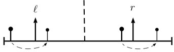 Figure 1
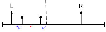 Figure 2
 Figure 3
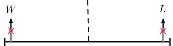 Figure 4
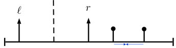 Figure 5
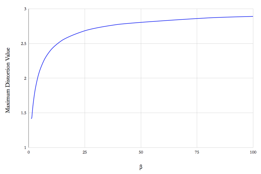 Figure 6
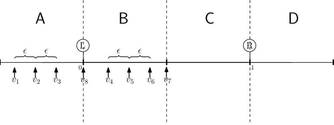 Figure 7
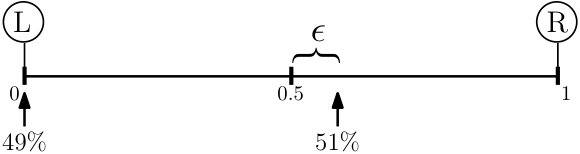 Figure 8
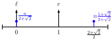 Figure 9
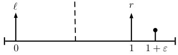 Figure 10
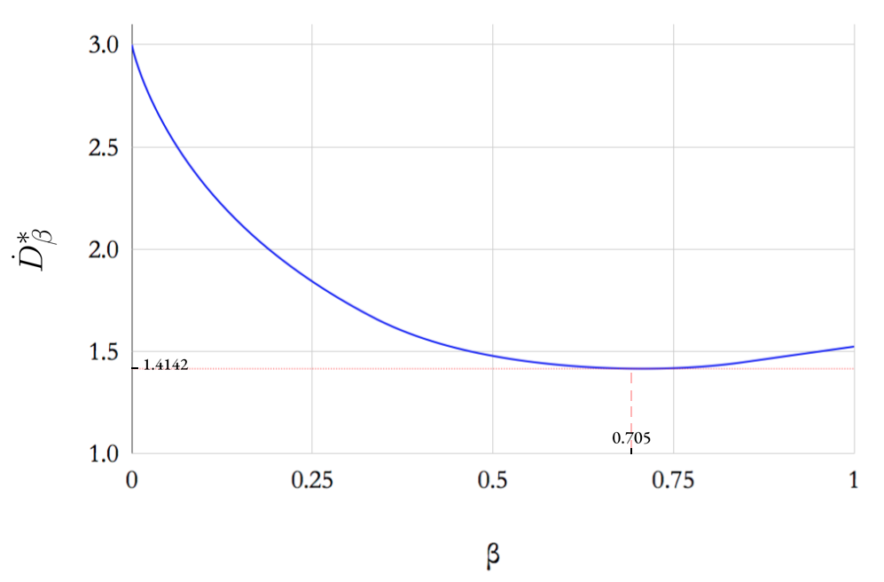 Figure 11
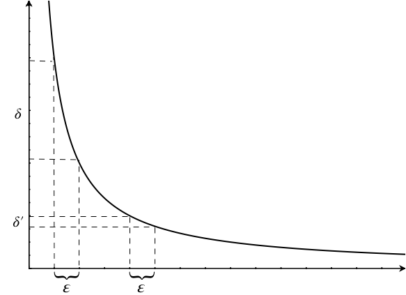 Figure 12
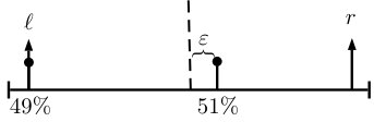 Figure 13
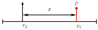 Figure 14
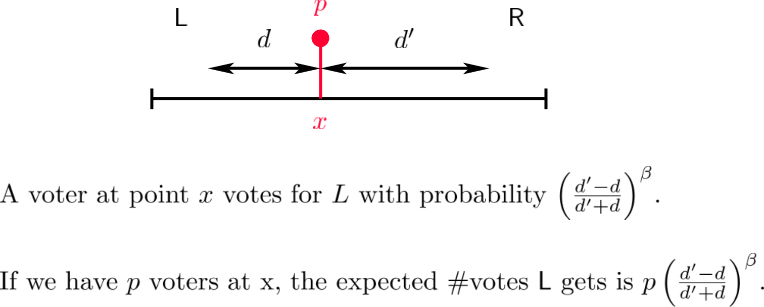 Figure 15
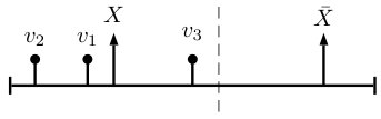 Figure 1
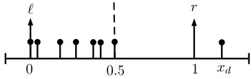 Figure 17
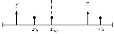 Figure 18
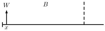 Figure 19
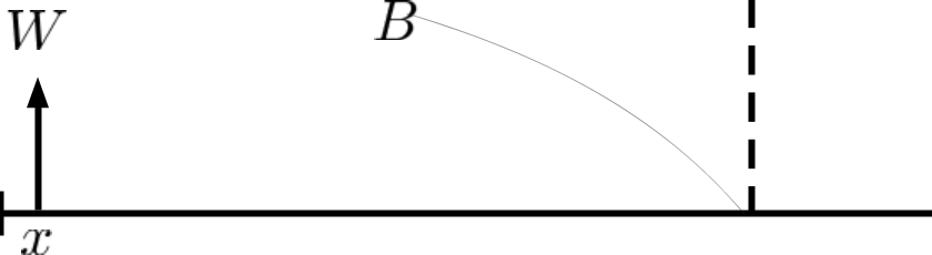 Figure 20
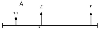 Figure 21
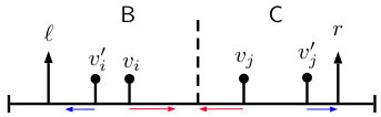 Figure 22
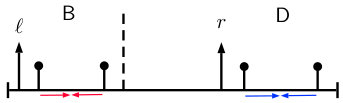 Figure 23
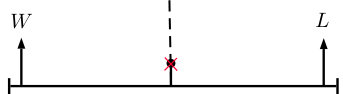 Figure 24
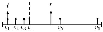 Figure 25
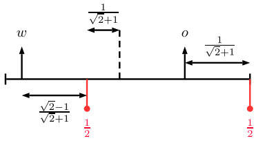 Figure 26
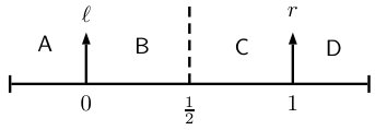 Figure 27
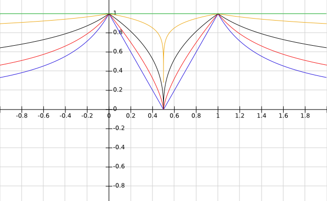 Figure 28
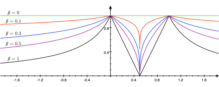 Figure 29
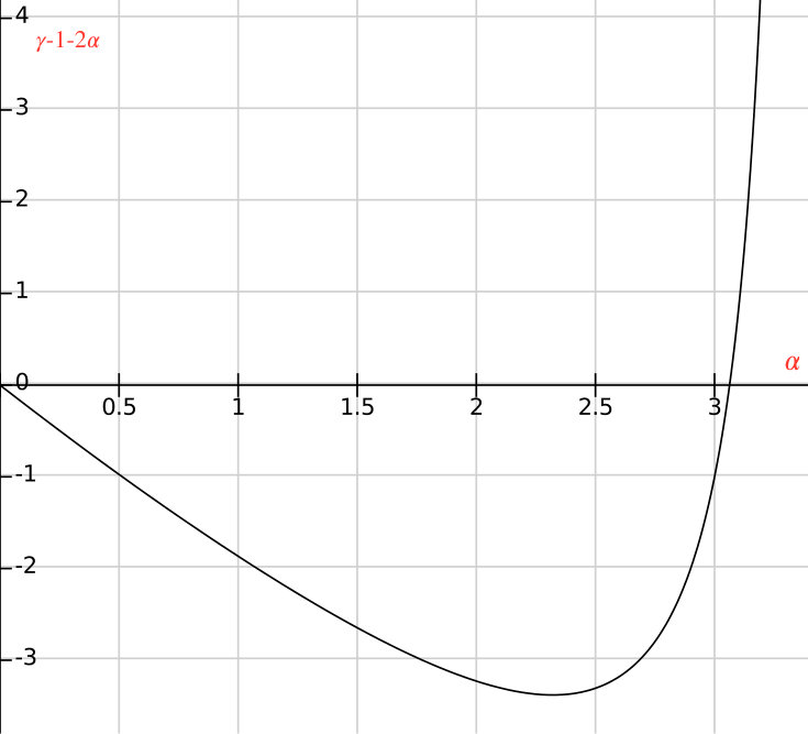 Figure 30
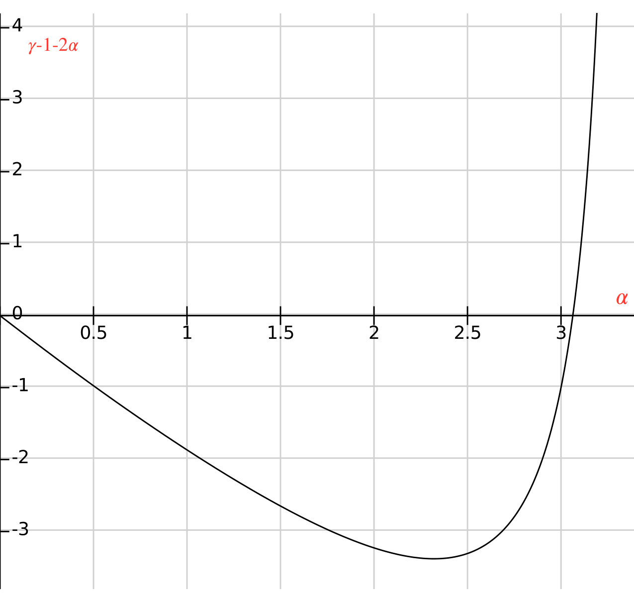 Figure 31
Peer Reviews
No public reviews on file for this paper yet. If you reviewed it on a platform where reviews are public (OpenReview, ICLR, NeurIPS, ICML), you can paste yours below so the community can read it here.
Videos
No videos yet. Explain this paper in a talk, walkthrough, or lecture? Add one.
On the Distortion Value of Elections with Abstention
Mohammad Ghodsi
Sharif University of Technology
Institute for Research in Fundamental Sciences (IPM)
Mohamad Latifian
Sharif University of Technology
Masoud Seddighin
Institute for Research in Fundamental Sciences (IPM)
Abstract
In Spatial Voting Theory, distortion is a measure of how good the winner is. It has been proved that no deterministic voting mechanism can guarantee a distortion better than , even for simple metrics such as a line. In this study, we wish to answer the following question: how does the distortion value change if we allow less motivated agents to abstain from the election?
We consider an election with two candidates and suggest an abstention model, which is a general form of the abstention model proposed by Kirchgässner [26]. Our results characterize the distortion value and provide a rather complete picture of the model. 111A preliminary version of this paper is accepted in AAAI 2019.
1 Introduction
The goal in Social Choice Theory is to design mechanisms that aggregate agents’ preferences into a collective decision. Voting is a well-studied method for aggregating preferences with many applications in artificial intelligence and multi-agent systems. Roughly, a voting mechanism takes the preferences of the agents over a set of alternatives and selects one of them as winner.
One fruitful approach to estimate the quality of a voting mechanism is to use the utilitarian view which assumes that each agent has cost over the alternatives [33, 11, 9, 7, 24, 6]. For example, spatial models locate the voters and the alternatives in a finite metric space , and the cost of voter for Alternative equals to their distance [4, 2, 3, 23, 8, 5, 28]. Considering these costs, the optimal candidate is defined to be the candidate that minimizes the social cost (the total cost of the voters). Ideally, we would like the optimal candidate to be the winner; however, since voting mechanisms only take the ordinal preferences of voters as input, it is reasonable to expect that the winner is not always optimal. The question then arises: how good is the winner, i.e., what is the worst-case ratio of the social cost of the winner to the social cost of the optimal candidate? This ratio is called the distortion value of a voting mechanism. It is known that no deterministic voting mechanism can guarantee a distortion better than , even for simple metrics such as a line [4]. To see this, consider the example shown in Figure 1. In this example, candidate is the optimal candidate, and under the plurality voting rule 222For two candidates, all the well-known deterministic voting mechanisms (e.g. Borda, -approval, Copeland, etc) turn into plurality. candidate is the winner. Thus, the distortion value is
[TABLE]
However, the example of Figure 1 seems unrealistic in some ways. Although the voters located near the point are closer to , they have a very low incentive to vote for , since their costs for both candidates are almost equal. On the other hand, agents located at [math] have a strong incentive to vote for . Indeed, if voters are allowed to abstain, which is a natural assumption in many real-world elections, we expect to be the winner rather than . In this study, our goal is to tackle this problem:
How does the distortion value change, if we allow less motivated agents to abstain?
1.1 Abstention
Scientists have long studied the factors affecting participation in an election. For example, Wolfinger and Rosenstone [19] argue that more educated voters participate with a higher probability, or Lijphart [27] discusses that the voters on the left side of the political spectrum participate less frequently. Similarly, the decision to vote may rely on variables such as income level or the sense of civic duty [37].
Traditionally, both game-theoretic and decision-theoretic models of turnout have been proposed. At the heart of most of these models lies the assumption that there are costs for voting.333There are other decision theoretic explanations of abstention that do not rely on costs, e.g., see [22]. These costs include the costs of collecting and processing information, waiting in the queue and voting itself. Presumably, if a voter decides to abstain, she does not have to pay these costs. Therefore, a rational voter must receive utility from voting. There is evidence suggesting that voters behave strategically when deciding to vote and take the costs and benefits into account. For example, Riker and Ordeshook [35] show that the turnout is inversely related to voting costs.
Apart from social-psychological traits, other studies suggest that voters’ abstention may stem from their ideological distances from the candidates. The work of Downs [16] initiated this line of research. He argues that in a two-candidate election under the majority rule, the choice between voting and abstaining is related to the voter’s comparative evaluation of the candidates. Riker and Ordeshook [35] later improve this model by reformulating the original equation to incorporate other social and psychological factors.
Many empirical studies in spatial theory of abstention suggest that the voters are more likely to abstain when they feel indifferent toward the candidates or alienated from them [26]. The models introduced by Downs [16] and Riker and Ordeshook [35] are only capable of explaining the indifference-based abstention which occurs when the difference between the costs of candidates for a voter is too small to justify voting costs. On the other hand, these models cannot justify alienation-based abstention, which occurs when a voter is too distant from the alternatives to justify voting costs. To alleviate this, some studies argue that the relative ideological distance plays a more critical role than the absolute distance [26, 21]. Our model of abstention in this paper a generalization of the model introduced by Kirchgässner [26] which incorporates the relative distances.
1.2 Our Work
In this paper, we consider the effect of abstention on the distortion value. In our study, there are two candidates, and the voters decide whether to vote or abstain based on a comparison between the cost (i.e., distance) of their preferred alternative and the cost of the other alternative. We define the concepts of expected winner and expected distortion to evaluate the distortion of an election in our model. Our results characterize the distortion value and provide a complete picture of the model. For the special case that our abstention model conforms exactly to that of Kirchgässner [26], we show that the distortion of the expected winner is upper bounded by .
We also give an almost tight upper bound on the expected distortion value of large elections. We show that for any and a large enough election (in term of the number of voters), the expected distortion is upper-bounded by , where is the distortion of the expected winner.
Finally, we generalize our results to include arbitrary metric spaces. We show that the same upper bounds obtained for the distortion value for the line metric also work for any arbitrary metric space.
1.3 Related Work
The utilitarian view, which assumes that the voters have costs for each alternative, is a well-known approach in welfare economics [36, 30] and has received attention from the AI community during the past decade [33, 9, 10, 32, 3, 12, 23, 25, 1, 11]. Procaccia and Rosenschein [33] first introduced distortion as a benchmark for measuring the efficiency of a social choice rule in utilitarian settings. The worst-case distortion of many social choice functions is shown to be high or even unbounded. However, imposing some mild constraints on the cost functions yields strong positive results. One of these assumptions which is reasonable in many political and social settings, is the spatial assumption which assumes that the agent costs form a metric space [17, 28, 20, 4, 2, 31, 29].
Anshelevich, Bhardwaj and Postl [4] were first to analyze the distortion of ordinal social choice functions when evaluated for metric preferences. For plurality and Borda rules, they prove that the worst-case distortion is , where is the number of alternatives. On the positive side, they show that for the Copeland rule, the distortion value is at most 5. They also prove the lower bound of 3 for any deterministic voting mechanism and conjecture that the worst-case distortion of Ranked Pairs social choice rule meets this lower-bound. This conjecture is later refuted by Goel, Krishnaswamy, and Munagala [23]. Recently, Munagala and Wang [29] present a weighted tournament rule with distortion of .
In addition to deterministic social choice rules, the distortion of randomized rules have been also studied in the literature. The output of such mechanisms is a probability distribution over the set of alternatives rather than a single winning alternative. Anshelevich and Postl [3] show that for -decisive metric spaces 444 In an -decisive metric, for every voter, the cost of her preferred choice is at most times the cost of her second best choice. any randomized rule has a lower-bound of on the distortion value. For the case of two alternatives, they propose an optimal algorithm with the expected distortion of at most . Cheng et al. [14] characterized the positional voting rules with constant expected distortion value (independent of the number of candidates and the metric space).
Chen, Dughmi, and Kempe [13] consider the case that candidates are drawn randomly from the population of voters. They prove the tight bound of for the distortion value in the line metric and an upper-bound of for an arbitrary metric space.
In addition to the studies mentioned in Section 1.1, there are many other studies that consider the effect of abstention in various types of elections. For example, Desmedt and Elkind in [15] propose a game theoretic analysis of the plurality voting with the possibility of abstention and characterize the preference profiles that admit a pure Nash equilibrium. Rabinovich et al. [34] consider the computational aspects of iterative plurality voting with abstention. Also, related to our work is the concept of embedding into voting rules introduced by Caragiannis and Procaccia [11]. An embedding is a set of instructions that suggests each agent how to vote, based only on the agent’s own utility function. For example, when the voting mechanism is majority, one possible embedding is that voters vote for each candidate with a probability which is proportion to their utility for that candidate. Among other results, Caragiannis and Procaccia [11] show that this embedding results in constant distortion. Indeed, our abstention model can be seen as a embedding for elections with majority rule where voters are allowed to abstain.
2 Preliminaries
In our study, every election consists of four ingredients:
- •
A set of voters. We denote the ’th voter by .
- •
A set candidates. In this study, we suppose that there are only two candidates and denote the candidates by (left candidate) and (right candidate). 555In few cases, we also use and to refer to the left and right candidates.
- •
A finite metric space where the candidates and the voters are located. Unless explicitly stated otherwise, we suppose that is a line, and and are located respectively at points [math] and . In addition, each voter is attributed a value which shows her location on the line. We denote by , the distance between voter and alternative .
- •
A mechanism by which the winner is selected. In this paper, we consider a simple scenario where the winning candidate is elected via the majority rule (in case of a tie, the winner is determined by tossing a fair coin). Note that for two candidates, almost all the well-known deterministic voting mechanisms select the candidate preferred by the majority as winner.
Definition 2.1**.**
For an election and candidate , we define the social cost of in as
[TABLE]
The optimal candidate of election , denoted by is the candidate that minimizes the social cost, i.e.,
[TABLE]
We suppose that each voter either abstains or votes for one of the candidates. In Section 2.1 we give a formal description of the voting behavior of the agents.
2.1 Voting Behavior of Individuals
We employ a simple probabilistic model, where each voter independently decides whether to abstain or participate by evaluating her distances from the candidates. Fix an election and a voter and let be the candidate closer to in and be the other candidate. We suppose that votes sincerely for her preferred candidate with a probability where is a function of and , and abstains with probability .
Denote by the probability function from which is derived, i.e., . Since represents the probability of voting, we expect to satisfy certain axiomatic assumptions. Recall that in spatial voting models, there are two crucial sources of abstention [26]:
- •
Indifference-based Abstention (IA): the smaller the difference between the distances of a voter from the candidates is, the less likely it is that she casts a vote.
- •
Alienation-based Abstention (AA): the further a voter is located from his preferred candidate, the less likely it is that she casts a vote.
To illustrate, for the voters in Figure 2, we have:
- •
Voters and prefer and voters and prefer .
- •
Voter has a strong incentive to cast a vote since her cost for is zero.
- •
Voter always abstains, since her costs for both the candidates are equal (IA).
- •
For voters and , we have , since is more alienated (AA).
- •
For voters and , we have , since , and (IA,AA).
As mentioned, the models of Downs [16] and Riker and Ordeshook [35] are only capable of explaining the Indifference-based abstention, since they only consider the absolute difference between the distances of the candidates to a voter. To resolve this, some recent studies argue that the relative distance, rather than absolute distance, is relevant. In this study, we follow the model of Kirchgässner [26] which is based on the relative distances. The idea is that the probability that a voter casts a vote depends on her ability to distinguish between the candidates. By Weber–Fechner’s law (see [18]), the ability to distinguish between the candidates depends on their relative distances to the voter. Formally, the probability that voter votes for is calculated via the following formula:
[TABLE]
Here we consider a more general form of Equation (1). We suppose that each voter in election casts a vote with probability , where
[TABLE]
where is a constant in . Figure 3 shows the behavior of for different values of and different locations on the line. As is clear from Figure 3, for the smaller values of , voters are more eager to participate. Indeed, the exponent can be seen as a quantitative measure of how much this ideological distance matters. For the special case of , voters always participate in the election, regardless of their location. We refer to as the participation parameter. It can be easily observed that for any , function satisfies all the desired criteria.
2.2 Expected Winner and Expected Distortion
As mentioned, our assumption is that the winner is determined by the majority rule. However, according to the stochastic behavior of the voters, the winner is not deterministic, i.e., each candidate has a probability of winning. Denote by , the expected number of voters who vote for candidate , when the participation parameter is . Furthermore, denote by , the probability that candidate wins the election, when the participation probability is . We define the expected winner of election for participation parameter , denoted by as the candidate with the maximum expected number of votes.
[TABLE]
Definition 2.2**.**
For election and a candidate we define the distortion of in election , denoted by , as the ratio
By definition, the distortion of the optimal candidate is . We discuss two approaches to evaluate the distortion of an election . In the first approach, we evaluate election by the distortion of its expected winner, i.e., . Another approach is to define the distortion of election as the expected distortion of the winner, over all possible outcomes, i.e.,
[TABLE]
Finally, for any , we define worst-case distortion values and as:
[TABLE]
and
[TABLE]
where is the set of all possible elections . We dedicate two separate sections to analyze the value of and . Even though the value of and essentially depend on , we provide necessary tools to analyze distortion these values for any .
For convenience, in the rest of the paper, when is fixed we drop the subscript ‘’ and simply use instead of
3 Distortion of the Expected Winner
Throughout this section, we analyze the worst-case distortion of the expected winner. Recall that the expected winner is the candidate with a higher expected number of votes. There are two reasons why we consider the distortion value of the expected winner. First, since the number of votes that each candidate receives is concentrated around its expectation 666We can show this claim using concentration bounds such as Hoeffding. A simple form of this inequality states that for independent random variables bounded by , we have
where is the sum of the variables. , in elections with a large number of voters, the expected winner has a very high chance of winning; especially when there is a non-negligible separation between the expected number of votes that each candidate receives. Secondly, we use the tight upper-bound on the distortion value of the expected winner to prove an upper bound on the expected distortion of the election for the second approach. Recall that the probability that a voter casts a vote for his favorite candidate in election is:
[TABLE]
In this section, we suppose without loss of generality that candidate is the expected winner. Moreover, we assume that the optimal candidate is ; otherwise the distortion equals . We also consider four regions and D as in Figure 4.
In Theorem 3.1 we state the main result of this section.
Theorem 3.1**.**
For any , there exists an election , such that and the voters in are located at two different locations and .
The basic idea to prove Theorem 3.1 is as follows: we prove that for every election , there exists an election with , such that the voters in are located in at most different locations. To show this, we collect the voters in by carefully moving them forward and backward via a sequence of valid displacements, as defined in Definition 3.2.
Definition 3.2**.**
Define a displacement as the operation of moving a subset of the voters forward or backward on the line to a new location. A displacement is valid if it does not alter the expected winner, and furthermore, does not decrease the distortion value of the expected winner.
In Lemmas 3.3, 3.4, and 3.5 we introduce three sorts of valid displacement which help us collect the voters. For convenience, here we only state the lemmas and defer the proofs to Section 3.2. Figure 5, illustrates a summary of the valid displacements introduced in these lemmas. Note that these displacements are valid for any .
Lemma 3.3**.**
Moving a voter from to [math] is a valid displacement.
Lemma 3.4**.**
Consider voters and respectively at and . Then,
- •
If , moving to and to is a valid displacement.
- •
If , moving to and to is a valid displacement.
Lemma 3.5**.**
Consider voters , where or . Then moving both the voters to is a valid displacement.
We also state two simple and natural Corollaries of Lemmas 3.4, and 3.5.
Corollary 3.6** (of Lemma 3.4).**
We can move each voter in region C to either or by a sequence of valid displacements.
Proof.
Consider an arbitrary voter . Since is the expected winner, there exists at least one voter, say , in region B. By Lemma 3.4, if , we can move to and if , we can move to . ∎
Corollary 3.7** (of Lemma 3.5).**
We can collect all the voters of region B at some point via a sequence of valid displacements. Furthermore, we can collect all the voters of region D at some point via a sequence of valid displacements.
Proof.
By applying Lemma 3.5 iteratively to the furthest voters, the maximum distance between the voters in each region decreases. This procedure can be applied until all the voters gather at one point. ∎
Now, we are ready to prove Theorem 3.1.
Proof of Theorem 3.1..
First, we prove that by Lemma 3.3 and Corollaries 3.6, and 3.7, every election can be reduced to an election , such that
- •
and have the same expected winner.
- •
.
- •
All the agents in are located at two points and .
Consider an arbitrary election . Using Lemma 3.3, we move all the voters in region A to [math]. Afterwards, using Corollary 3.6 we move each voter in region C to one of the points or . At this point, all the voters belong to one of regions B or D (we suppose that the voters located in the borderlines belong to both regions). Finally, using Corollary 3.7, we collect all the voters in regions B and D at some points .
Finally, let be an arbitrary election such that . Applying the above reduction on , yields an election with , and the desired structure. ∎
According to Theorem 3.1, for any , we can establish an election with the maximum distortion, and the following structure (see Figure 6): the interior of regions A and C contain no voter. All the voters are located at two points and . Note that, the maximum distortion value and the location of and in the worst-case scenario depends on the value of .
3.1 A Tight Upper Bound on
We now evaluate for different values of . Let us start by the boundary case . For , the probability that a voter casts a vote is independent of her location. It is proved that for this case, we have [4]. Indeed, the same example we provided in Figure 1 is the scenario with the highest distortion for .
Now, consider , and let be the election that maximizes . As discussed in the previous section, we can assume without loss of generality that the voters in are located at two points, namely, and . Suppose that voters are at and voters are at . We have:
[TABLE]
Since is the expected winner, we have
[TABLE]
On the other hand, we have
[TABLE]
and
[TABLE]
Thus,
[TABLE]
Therefore, in order to find the maximum distortion value, we need to solve the following optimization problem:
{maxi}qbxb+ (n-qb) xdqb(1-xb) + (n-qb)(xd- 1)\addConstraint
(1-2x_b)^βq_b ≥n-qb(2xd-1)β \addConstraint0 ≤q_b≤1 \addConstraint0 ≤x_b ≤1/2 \addConstraint1 ≤x_d.
Now consider another boundary case: . For the answer to the above optimization problem is , which can be obtained by choosing , , and . A graphical representation of this construction is shown in Figure 7.
In general for , the maximum distortion value equals the answer of Optimization Problem (3.1). In Figure 8, we show the answer of this program for different values of . Interestingly, with increasing from [math] to , initially decreases and then increases. As illustrated in Figure 8, it can be seen that the minimum possible value for is for .
3.2 Valid Displacements
In this section, we prove Lemmas 3.3, 3.4, and 3.5. One important tool to prove these lemmas is Observation 3.8.
Observation 3.8**.**
Let be four positive constants. We have :777For the second inequalities, we assume .
- •
If then and .
- •
If then and .
See 3.3
Proof.
Initially, votes for with probability . After moving to [math], she votes for with probability . Therefore, if we move to [math], the value of does not decrease, and the expected winner does not change. Furthermore, by this movement both and are decreased by . Let and be the contribution of (that is, all voters except ) to the social cost of and respectively. Before moving to [math], we have
[TABLE]
and after the movement we have
[TABLE]
By applying Observation 3.8 on Equation (4), we have
[TABLE]
which implies that moving to [math] is a valid displacement. ∎
See 3.4
Proof.
Initially, votes for with probability , and votes for with probability . Since these movements do not change the regions where the voters belong, after the movement they vote for the same candidate but with different probabilities. Let be the difference between the contribution of to , before and after the displacement. Similarly, let be the difference between the contribution of to before and after the movement. We consider two cases.
Case I (): if we move to and to , votes for with probability and votes for with probability [math]. Thus, we have
[TABLE]
Since , by straightforward calculus we have:
[TABLE]
Case II (): if we move to and to , after the displacement, votes for with probability and votes for with probability . Therefore, we have
[TABLE]
Since , we have
[TABLE]
Hence the expected winner does not change. In addition, since we move two voters in Regions B and C equally in the opposite directions in both cases, the distortion value of each candidate remains unchanged. ∎
See 3.5
Proof.
Let . Recall the definition of and from the proof of Lemma 3.4. For the case of , we have:
[TABLE]
and
[TABLE]
Thus, we have
[TABLE]
Since , these two inequalities imply (see Figure 9). Thus, value of does not increase and the expected winner does not change.
Similarly For the case of , we have:
[TABLE]
and
[TABLE]
Thus, we have
[TABLE]
Note that since is a decreasing and concave function, we have
[TABLE]
and
[TABLE]
Since , these two inequalities imply . Thus, value of does not decrease and the expected winner does not change. In addition, since the voters move in the opposite directions and by the same distance, the distortion value of the candidates do not change. Therefore, this modification is a valid displacement.
∎
4 Expected Distortion
Recall that in our second approach, we define the distortion of an election as the expected distortion of the winner, where the expectation is taken over the random behavior of the voters. Our main result in this Section is Theorem 4.1.
Theorem 4.1**.**
For any , value of for every election whose candidates receive at least
[TABLE]
expected number of votes is at most .
In this section, we suppose without loss of generality that candidate is the optimal candidate. Thus, Equation (3) can be rewritten as
[TABLE]
In this case, if would be the expected winner, we have:
[TABLE]
In addition, we know that the distortion of the expected winner is at most , which together with Equation (6) implies for the case that is the expected winner. Therefore, throughout this section we suppose that is both the optimal and the expected winner candidate.
In Theorem 4.2, we prove that there is an election with the maximum distortion value and a simple structure.
Theorem 4.2**.**
For any , there exists an election such that is maximum, and in there is no voter in the interior of regions A and C, and also all the voters in D are located at a single point .
The basic idea to prove Theorem 4.2 is as follows: we prove that for every election , there exists an election with and the desired structure. To show this, we collect some of the the voters in via a sequence of valid displacements, albeit with a new definition for valid displacement.
Definition 4.3**.**
A displacement is valid, if it does not decrease .
The process of proving that a displacement is valid for this case is relatively tougher than the previous model. The reason is that we do not even have a closed-form expression which represents the winning probability of each candidate. In Lemmas 4.4 and 4.5 we explain our tools to discover valid displacements. For brevity, we defer the proofs to these lemmas to Section 4.2.
Lemma 4.4**.**
For each voter , there is a point such that moving to is a valid displacement. Furthermore, for each voter , there is a point such that moving to is a valid displacement.
Lemma 4.5**.**
Let and be two voters located respectively at . Then, there exists a point between and , such that moving both the voters to is a valid displacement.
Figure 10, shows a summary of the displacements described in Lemmas 4.4 and 4.5. Using these displacements, one can establish an election with the maximum expected distortion, and the following structure (see Figure 11): the interior of regions A and C contain no voter. All the voters in D are located at point .
Proof of Theorem 4.2.
Consider an election with the maximum expected distortion. By Lemma 4.4 we can suppose that the interior of regions A and C are empty. Furthermore, by iteratively applying Lemma 4.5 on the farthest pair of points in Region D, we can collect all the voters of D into a single point and transform the election into one with the maximum distortion, and the desired structure.
∎
4.1 An Almost Tight Bound on
In this section, we discuss the value of , for any . As mentioned, to prove our upper and lower bounds in this section, we use the bounds obtained in Section 3.1.
Similar to Section 3.1, we begin with the boundary case of . By a similar argument as in Section 3.1, for all the voters vote for their preferred candidate and so we have . For , we prove Theorem 4.1 which provides an asymptotic upper bound on for any .
See 4.1
To prove Theorem 4.1, we first prove Lemmas 4.6 and 4.7.
Lemma 4.6**.**
Let be a constant, and be an election, with the property that is the optimal and the expected winner candidate, and . Then
Proof.
To prove this lemma we add sufficient number of agents at point [math] to alter the expected winner to . After this operation, since is the expected winner, we know that the expected distortion of is at most . Next, based on the number of voters added at point [math], we bound the value of .
Let be the minimum number of voters we need to add at point [math] to convert to the expected winner. Since , and each voter at point [math] contributes to , we have Let be the election, after adding the agents at point [math]. Since the expected winner of is , the expected distortion of is upper bounded by :
[TABLE]
Moreover, since we add the agents at point [math], their cost for candidate is zero and hence, . Thus, we have
[TABLE]
Now, we show that the ratio is upper bounded by . First, let us calculate the explicit formulas of and . As discussed before, we can assume that the agents in are located either in Region B or at point . Let be the population of the voters that are located at . We have
[TABLE]
Furthermore, we have where
[TABLE]
Thus, we have
[TABLE]
and since for any we have ,
[TABLE]
Inequality (9) together with Equations (7) and (8) implies:
[TABLE]
Thus, by Equation (5), we have
[TABLE]
and since we conclude that ∎
Lemma 4.7**.**
Let be a constant, and be an election, with the property that is the optimal and the expected winner candidate, and . Then, if the number of candidates would be large enough, we have .
Proof.
To prove Lemma 4.7, we use the fact that the number of votes that a candidate receives is concentrated around it’s expected value. By definition, we have
[TABLE]
Let and be two random variables indicating the number of votes that and receive in , respectively. These two variables are the sum of i.i.d. Bernoulli variables each indicating whether a voter casts a vote or not. Note that all the voters that contribute to are located at the same point, but voters contributing to might have different locations. Using these facts we can calculate the expected value and the variance of and . We have:
[TABLE]
Let . Since , we have
[TABLE]
Now, since we know both the expected value and the variance of and we can use Chebyshev’s inequality to provide an upper bound on .
Chebyshev’s inequality states that for a random variable with finite expected value and finite non-zero variance , and for any real number ,
[TABLE]
Therefore we have:
[TABLE]
On the other hand,
[TABLE]
Let
[TABLE]
Putting Equations (11), (13) and (14) together we have:
[TABLE]
and by Equation (10) we have:
[TABLE]
Note that since is the only location more distant to than , even for the distortion of candidate and consequently the distortion of the election is upper-bounded by . Therefore, if , the distortion of the election is upper bounded by (i.e. ). So here we assume . If we substitute for in (15) we have:
[TABLE]
where the last line is due to the fact that
[TABLE]
Now, suppose that the the expected number of votes that each candidate receives is large enough, so that
[TABLE]
By Equation (16) we have:
[TABLE]
This completes the proof. ∎
Now, we are ready to prove Theorem 4.1.
Proof of Theorem 4.1..
Fix any and , and let be an arbitrary election whose candidates receive at least
[TABLE]
expected number of votes. Recall that our assumption is that is both the optimal and the expected winner. Now, based on the value of , there are two cases: either or . For the first case, by Lemma 4.6 value of is upper bounded by . For the second case, since
[TABLE]
by Lemma 4.7, the expected distortion is upper bounded by . Combining these two cases yields the upper-bound of on . ∎
As an example, for , Theorem 4.1 states that for every election whose candidates receive at least expected number of votes, the expected distortion is upper bounded by which for is .
We complement Theorem 4.1 by describing how to construct bad examples with expected distortion value near .
Example 1**.**
Consider Optimization Problem 3.1, with an additional constraint that for a fixed constant , and let be the answer of this optimization problem and be its corresponding election. By Chernoff bound, for a large enough value of , candidate wins the election with a high probability, i.e.,
[TABLE]
Note that, the bound provided by Theorem 4.1 is almost tight; as the election size grows, the upper bounds of Theorem 4.1 tends to the distortion value of Example 1. However, for elections with a small number of voters, the distortion value might be larger. For example, consider a simple scenario where there is one voter located at point and (see Figure 12). For this case, the distortion value is
[TABLE]
which tends to as . We conjecture that this example is the worst possible scenario and value of is upper bounded by for any election with any size while .
4.2 Valid Displacements
In this section, we prove Lemmas 4.4 and 4.5. See 4.4
Proof.
We prove the statement of Lemma 4.4 for regions A and B. Similar arguments can be used to prove the lemma for regions C and D. Let be the current location of in region A (). By definition, casts a vote with probability Now, consider point . We claim that an agent at , votes for with the same probability as . First, note that since ,
[TABLE]
Hence, the preferred candidate of the voter located at is . Furthermore, for any agent at , the probability of casting a vote is
[TABLE]
Therefore, by moving from to , the probability that votes for remains the same. Let be the election, after moving to . We have
[TABLE]
Since we have
[TABLE]
using Observation 3.8 we conclude that which in turn implies that moving to is a valid displacement. ∎
See 4.5
Proof.
Assume without loss of generality that . We show that we can move both the voters to point
[TABLE]
Let be a random variable which is equal to , if casts a vote and [math] otherwise. In addition, let
[TABLE]
where . Trivially, we have , and
[TABLE]
Furthermore, note that we have
[TABLE]
Let and be variables indicating whether and cast a vote or not, after the displacement. We have
[TABLE]
Thus, we have
[TABLE]
Now, we show
[TABLE]
We have
[TABLE]
Since we just need to show
[TABLE]
which is trivial due to the fact that
[TABLE]
Furthermore, since
[TABLE]
we have
[TABLE]
Considering Equation (17), and the fact that we conclude that after this movement, the value of decreases and the value of increases.
Finally, let and be the cost of the agents other than and for and , respectively. By definition, before the displacement, we have
[TABLE]
and after moving and to point , we have:
[TABLE]
Again, by straightforward calculus, one can easily verify that
[TABLE]
Thus, after this displacement, both and increases, and so does the value of . ∎
5 General Metric
We now extend our results to general metric spaces. Suppose that the voters and candidates are located in an arbitrary metric . By definition, for every voter and candidates we have:
- •
.
- •
(triangle inequality).
We suppose without loss of generality that . For this case, we prove Theorem 5.1, which states that for every , the same upper bounds we obtained on the distortion value for the line metric also works for any arbitrary metric space.
Theorem 5.1**.**
For every election in an arbitrary metric space, there exists an election in line metric, such that and .
Proof.
Let be an election in an arbitrary metric space . Assume w.l.o.g. that candidate is the optimal candidate and let be the set of voters in election . For each voter , let . Based on the value of , we partition the voters into two subsets and , where
[TABLE]
[TABLE]
Now, we construct election as follows: consider a line and two candidates located respectively at [math] and . For each voter , we consider a voter in , located at point Since
[TABLE]
both and participate in their corresponding elections with equal probabilities. Similarly, for each voter , we consider a voter located at point Again, it can be observed that
[TABLE]
In conclusion, for every , voters and cast a vote in their corresponding elections with equal probabilities. Thus, expected winners of and are the same, and we have
[TABLE]
Now, we prove . For convenience, let
[TABLE]
[TABLE]
[TABLE]
[TABLE]
Note that for each , , , and . Hence and . Therefore we have and . In addition,
[TABLE]
On the other hand, for each , , , and . Hence and . Therefore we have and . Furthermore, we have:
[TABLE]
By Equations (19) and (20), and using Observation 3.8 we have
[TABLE]
and
[TABLE]
Since the expected winner is the same in and , Inequality (22) immediately implies that Furthermore, considering Equations (3) ,(18), and (22) we have ∎
6 Future Directions
In this study, we analyzed the distortion value in a spatial voting model with two candidates, when the voters are allowed to abstain. The set of results in this paper provides a rather complete picture of the model. Nevertheless, some important open questions remain open.
- •
The most immediate open question is to analyze the expected distortion value of the elections for a small number of voters. The counter-example in Section 4.1 refutes the existence of an upper bound better than . We believe that this example is the worst possible scenario. However, we don’t have a formal proof for this claim.
- •
Another direction is to provide a closed-form expression for the distortion of the expected winner. Currently, the maximum distortion is obtained via a mathematical program, which is not even convex 888Of course, we have a short note on how to reduce this program into a convex one, by eliminating some of the variables..
Beyond the above direct questions, this research also initiates an interesting line of work and opens a fruitful direction for the future research. In the following, we discuss two of these directions:
- •
In this paper, we focused on a majority election between two candidates. When more than two candidates are running, vote aggregation becomes more complex. One interesting direction is to generalize the models in this paper for elections with more than two candidates and analyze the performance of different well-established voting mechanisms such as Borda, -approval, Veto, Ranked pairs, and Copland under abstention assumption. One can also consider abstention in evaluating the distortion of different randomized mechanisms.
- •
Similar to the elections with no abstention, it seems that high distortion scenarios stem from the issue of representativeness of candidates. Cheng et. al. [14] show that when the candidates are of the people (i.e., they have the same distribution as the voters), distortion ratio improves to a constant upper-bound strictly better than for general metrics. The question is, how does the distortion value change if we allow abstention in the societies that voters and candidates have the same distribution?
The reference list from the paper itself. Each links out to its DOI / PubMed record.
- 1Amanatidis et al. [2020] G. Amanatidis, G. Birmpas, A. Filos-Ratsikas, and A. A. Voudouris. Peeking behind the ordinal curtain: improving distortion via cardinal queries. In Thirty-Fourth AAAI Conference on Artificial Intelligence , 2020.
- 2Anshelevich [2016] E. Anshelevich. Ordinal approximation in matching and social choice. ACM SI Gecom Exchanges , 15(1):60–64, 2016.
- 3Anshelevich and Postl [2017] E. Anshelevich and J. Postl. Randomized social choice functions under metric preferences. Journal of Artificial Intelligence Research , 58:797–827, 2017.
- 4Anshelevich et al. [2018] E. Anshelevich, O. Bhardwaj, E. Elkind, J. Postl, and P. Skowron. Approximating optimal social choice under metric preferences. Artificial Intelligence , 264:27–51, 2018.
- 5Barberà et al. [1993] S. Barberà, F. Gul, and E. Stacchetti. Generalized median voter schemes and committees. Journal of Economic Theory , 61(2):262–289, 1993.
- 6Benade et al. [2017] G. Benade, S. Nath, A. D. Procaccia, and N. Shah. Preference elicitation for participatory budgeting. In Thirty-First AAAI Conference on Artificial Intelligence , 2017.
- 7Benade et al. [2019] G. Benade, A. D. Procaccia, and M. Qiao. Low-distortion social welfare functions. In Proceedings of the 33rd AAAI Conference on Artificial Intelligence. , 2019.
- 8Black [1948] D. Black. On the rationale of group decision-making. Journal of political economy , 56(1):23–34, 1948.