The Online Event-Detection Problem

TL;DR

This paper introduces the online event-detection problem (OEDP), focusing on real-time identification of specific frequency-based events in data streams with strict accuracy and timeliness requirements, and proposes cache-efficient algorithms for it.

Contribution

The paper formulates the OEDP, proves its space complexity, and develops near-optimal cache-efficient algorithms with tunable parameters for false positives and reporting delay.

Findings

Algorithms are within a log factor of optimal in external memory.

The algorithms can be tuned for bounded false positives and delays.

Improved performance when input follows a power-law distribution.

Abstract

Given a stream $S = (s_1, s_2, ..., s_N)$, a $\phi$-heavy hitter is an item $s_i$ that occurs at least $\phi N$ times in $S$. The problem of finding heavy-hitters has been extensively studied in the database literature. In this paper, we study a related problem. We say that there is a $\phi$-event at time $t$ if $s_t$ occurs exactly $\phi N$ times in $(s_1, s_2, ..., s_t)$. Thus, for each $\phi$-heavy hitter there is a single $\phi$-event which occurs when its count reaches the reporting threshold $\phi N$. We define the online event-detection problem (OEDP) as: given $\phi$ and a stream $S$, report all $\phi$-events as soon as they occur. Many real-world monitoring systems demand event detection where all events must be reported (no false negatives), in a timely manner, with no non-events reported (no false positives), and a low reporting threshold. As a result, the OEDP requires a large amount of space (Omega(N) words) and is not solvable in the streaming model or via standard sampling-based approaches. Since OEDP requires large space, we focus on cache-efficient algorithms in the external-memory model. We provide algorithms for the OEDP that are within a log factor of optimal. Our algorithms are tunable: its parameters can be set to allow for a bounded false-positives and a bounded delay in reporting. None of our relaxations allow false negatives since reporting all events is a strict requirement of our applications. Finally, we show improved results when the count of items in the input stream follows a power-law distribution.

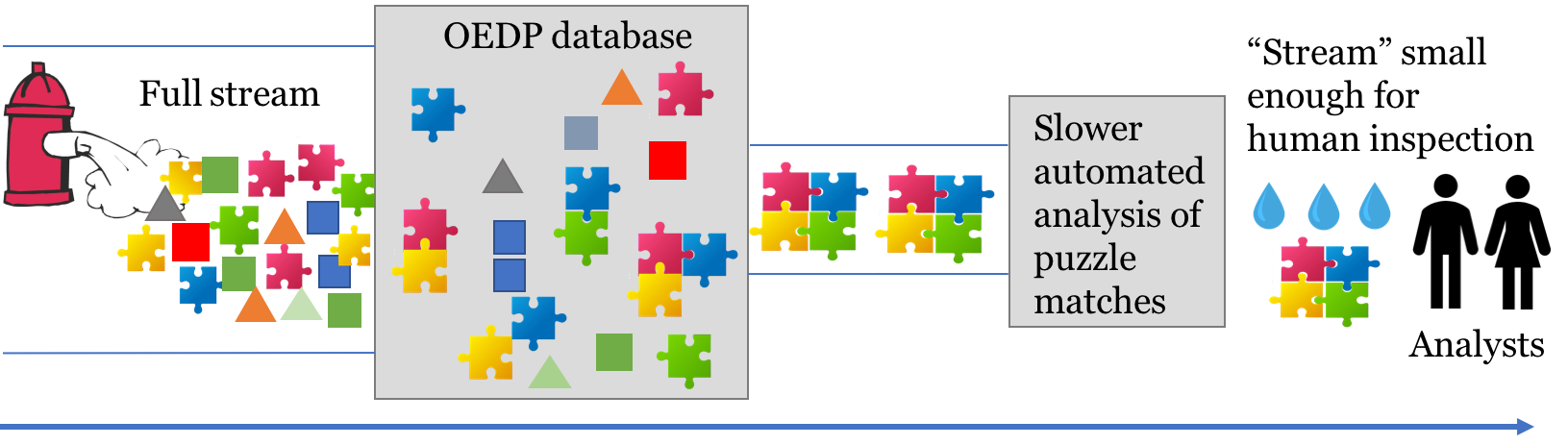Figures

Equations

$$\displaystyle 1=\int_{1}^{\infty}p(x)\,dx=Z\int_{1}^{\infty}x^{-\theta}\,dx=\frac{Z}{\theta-1}\Big{[}\frac{-1}{x^{\theta-1}}\Big{]}_{1}^{\infty}=\frac{Z}{\theta-1}.$$

$$\text{mbox}Prob(x>c)$$

$$\displaystyle=\big{[}-x^{-\theta+1}\big{]}_{c}^{\infty}=\frac{1}{c^{\theta-1}}.$$

$$\le \frac{N}{{({\sum }_{\ell =L}^{i+2}{\tau }_{\ell })}^{\theta -1}}<\frac{N}{{{\tau }_{i+2}}^{\theta -1}}.$$

$$\frac{N}{{{\tau }_{i+2}}^{\theta -1}}\le \frac{1}{\epsilon r^{L-i-1}}.$$

$$\frac{N}{{({\sum }_{\ell =L}^{i+1}{\tau }_{\ell })}^{\theta -1}}$$

$$=\frac{1}{r}\cdot \frac{N}{({{\tau }_{i+2}}^{\theta -1})}\le \frac{1}{r\epsilon r^{L-i-1}}=\frac{1}{r^{L-i}\epsilon }.$$

Full text

Many real-world monitoring systems demand event detection where all events must be reported (no false negatives), in a timely manner, with no non-events reported (no false positives), and a low reporting threshold. As a result, the oedp requires a large amount of space ($\Omega(N)$ words) and is not solvable in the streaming model or via standard sampling-based approaches.

Since oedp requires large space, we focus on cache-efficient algorithms in the external-memory model.

We provide algorithms for the oedp that are within a log factor of optimal. Our algorithms are tunable: their parameters can be set to allow for bounded false-positives and a bounded delay in reporting. None of our relaxations allow false negatives since reporting all events is a strict requirement for our applications. Finally, we show improved results when the count of items in the input stream follows a power-law distribution.

1 Introduction

Real-time monitoring of high-rate data streams, with the goal of detecting and preventing malicious events, is a critical component of defense systems for cybersecurity [47, 39, 50] and physical systems, such as water or power distribution [15, 36, 40]. In such a monitoring system, changes of state are inferred from the stream elements. Each detected/reported event triggers an intervention. Analysts use more specialized tools to gauge the actual threat level. Newer systems are even beginning to take defensive actions, such as blocking a remote host, automatically based on detected events [43, 34]. When used in an automated system, accuracy (i.e., few false-positives and no false-negatives) and timeliness of event detection are essential.

Motivated by these applications, we define and study the online event-detection problem (oedp). Roughly speaking, the oedp seeks to report all anomalous events (events that cross a predetermined safety threshold) as soon as they occur in the input stream. The related problem of finding the most frequent elements or heavy hitters in streams has been extensively studied in the database literature [29, 30, 4, 24, 19, 18, 38, 16, 32, 42, 17, 31, 17, 14]. More formally, given a stream $S=(s_{1},s_{2},\ldots,s_{N})$, a $\phi$-heavy hitter is an element $s$ that occurs at least $\phi N$ times in $S$. Here we focus on the problem of finding $\phi$-events, where we say that there is a $\phi$-event at time step $t$ if $s_{t}$ occurs exactly $\lceil\phi N\rceil$ times in $(s_{1},s_{2},\ldots,s_{t})$. Thus for each $\phi$-heavy hitter there is a single $\phi$-event which occurs when its count reaches the reporting threshold $T=\lceil\phi N\rceil$.

Formally, we define the online event-detection problem (oedp) as: given stream $S=(s_{1},s_{2},\ldots,s_{N})$, for each $i\in[1,N]$, report if there is a $\phi$-event at time $i$ before seeing $s_{i+1}$. A solution to the online event-detection problem must report

1. (a)

all events111We drop the $\phi$ when it is understood. (no False Negatives) 2. (b)

with no non-events and no duplicates (no False Positives) 3. (c)

as soon as an element crosses the threshold (Online).

Furthermore, an online event detector must scale to

1. (d)

small reporting thresholds $T$ and large $N$, i.e., very small $\phi$ (Scalable).

In this paper, we present algorithms for the oedp. We also give solutions which relax conditions (b) and (c). However, our solutions are motivated by cybersecurity applications where (a) and (d) are strict requirements. Next, we discuss how each of these conditions relate to our approach and results. See Section 6 for more details about the application that motivates the oedp and its constraints.

No false negatives. We are motivated by monitoring systems for national security [1, 5]. The events in this context have especially high consequences so it is worth investing extra resources to detect them. We therefore do not allow false negatives (i.e., condition (a) is strict); see Section 6 for more details. This rules out sampling-based approaches for the oedp, which necessarily incur false negatives.

Scalability. Scalability (condition (d)) is essential in the broader context of detecting anomalies in network streams, since anomalies are often small-sized events that develop slowly, appearing normal in the midst of large amounts of legitimate traffic [41, 49]. As an example of the demands placed on event detection systems, the US Department of Defense (DoD) and Sandia National Laboratories developed the Firehose streaming benchmark suite [1, 5] to measure the performance of oedp algorithms. In the FireHose benchmark, the reporting threshold is preset to the representative value of $T=24$, which translates to $\phi=24/N=o(1)$ and thus a DoD benchmark enforces condition (d).

Scalable solutions to the oedp require a large amount of space, ruling out the streaming model [6, 51], where the available memory is small—usually just $\mbox{polylog}(N)$. In particular, streaming algorithms for the heavy-hitters problem assume $\phi>1/\mbox{polylog}(N)$ (all candidates must fit in memory). Even if some false positives are allowed, as in the $(\varepsilon,\phi)$-heavy hitters problem222Given a stream of size $N$ and $1/N\leq\varepsilon<\phi\leq 1$, report every item that occurs $\geq\phi N$ times and no item that occurs $\leq(\phi-\varepsilon)$ times. It is optional whether to report items with counts between $(\phi-\varepsilon)N$ and $\phi N$., Bhattacharyya et al. [16] proved a lower bound of $(1/\varepsilon)\log(1/\phi)+(1/\phi)\log|{\mathcal{}U}|+\log\log N$ bits. Thus the space requirement is large when $\varepsilon$ is small, as is the case for Scalable solutions where $\phi$ is small, since $\varepsilon<\phi$.

Bounded false positives. Our algorithms for the oedp are tunable: parameters can be set to allow bounded false positives (relaxing condition (b)). We show that allowing some false positives results in fewer I/Os per element.

Allowing False Positives does not lead to substantial space savings. If we allow $O(1+\beta t)$ false positives in a stream with $t$ true positives, for any constant $\beta$, a bound of $\Omega(N\log N)$ bits follows via a standard communication-complexity reduction from the probabilistic indexing problem [48, 37]. Besides, as argued above, Scalable solutions to the heavy-hitter problem require large space even when False Positives are allowed.

Bounded reporting delay. The national-security monitoring systems we are interested in (see Section 6) can tolerate a slight delay in reporting when the high-risk event gives sufficient warning for intervention. We show that allowing a bounded delay in reporting (relaxing condition (c)) allows us to circumvent the lower bounds on $\phi$ imposed by our online solution. Thus, bounded delay is especially desirable when we want our oedp algorithm to scale to arbitrarily small reporting thresholds.

Finally, we note that in a security setting like ours, all events need to be detected in real-time to mitigate the associated risk. Thus streaming algorithms for the heavy-hitter problem that require multiple passes over the data are not applicable.

Online Event Detection in External Memory

In this paper, we make the large space requirement ($\Omega(N)$ words) of the oedp more palatable by shifting most of the storage from expensive RAM to lower-cost external storage, such as SSDs or hard drives. In particular, we give cache-efficient algorithms for the oedp in the external-memory model. In the external-memory model, RAM has size $M$, storage has unbounded size, and any I/O access to external memory transfers blocks of size $B$. Typically, blocks are large, i.e., $B>\log N$ [33, 3].

At first, it may appear trivial to detect heavy hitters using external memory: we can store the entire stream, so what is there to solve? And this would be true in an offline setting. We could find all events by logging the stream to disk and then sorting it.

The technical challenge to online event detection in external memory is that searches are slow. A straw-man solution is to maintain an external-memory dictionary to keep track of the count of every item, and to query the dictionary after each stream item arrives. But this approach is bottlenecked on dictionary searches. In a comparison-based dictionary, queries take $\Omega(\log_{B}N)$ I/Os, and there are many data structures that match this bound [26, 7, 22, 9]. This yields an I/O complexity of $O(N\log_{B}N)$. Even if we use external-memory hashing, queries still take $\Omega(1)$ I/Os, which still gives a complexity of $\Omega(N)$ I/Os [35, 27]. Both these solutions are bottlenecked on the latency of storage, which is far too slow for stream processing.

Data ingestion is not the bottleneck in external memory. Optimal external-memory dictionaries (including write-optimized dictionaries such as $B^{\varepsilon}$-trees [22, 11], COLAs [10], xDicts [21], buffered repository trees [23], write-optimized skip lists [13], log structured merge trees [46], and optimal external-memory hash tables [35, 27]) can perform inserts and deletes extremely quickly. The fastest can index using $O\!\left(\frac{1}{B}\log{\frac{N}{M}}\right)$ I/Os per stream element, which is far less than one I/O per item. In practice, this means that even a system with just a single disk can ingest hundreds of thousands of items per second. For example, at SuperComputing 2017, a single computer was easily able to maintain a $B^{\varepsilon}$-tree [22] index of all connections on a 600 gigabit/sec network [8]. The system could also efficiently answer offline queries. What the system could not do, however, was detect events online.

In this paper, we show how to achieve online (or nearly online) event detection for essentially the same cost as simply inserting the data into a $B^{\varepsilon}$-tree or other optimal external-memory dictionary.

Results

As our main result, we present an external-memory algorithm that solves the oedp, for $\phi$ that is sufficiently large, at an amortized I/O cost that is substantially cheaper than performing one query for each item in the stream.

Result 1**.**

Given a stream $S$ of size $N$ and $\phi>1/M+\Omega(1/N)$, the online event-detection problem can be solved at an amortized cost of $O\left(\left(\frac{1}{B}+\frac{M}{(\phi M-1)N}\right)\log\frac{N}{M}\right)$ I/Os per stream item.

To put this in context, suppose that $\phi>1/M\mbox{ and }(\phi>B/N\mbox{ or }N>MB)$. Then the I/O cost of solving the oedp is $O\!\left(\frac{1}{B}\log\left({\frac{N}{M}}\right)\right)$, which is only a logarithmic factor larger than the naïve scanning lower bound. In this case, we eliminate the query bottleneck and match the data ingestion rate of $B^{\varepsilon}$-trees.

Our algorithm builds on the classic Misra-Gries algorithm [28, 44], and thus supports its generalizations. In particular, similar to the $(\varepsilon,\phi)$-heavy hitters problem, our algorithm can also be relaxed so that items with frequency between $(\phi-\varepsilon)N$ and $\phi N$ may be reported. Allowing false positives lowers the amortized I/O cost to $O\left(\left(\frac{1}{B}+\frac{M}{(\phi M-1)N}\right)\log\frac{1}{\varepsilon M}\right)$; see Theorem 1. For the oedp (i.e., no False Positives), we set $\varepsilon=1/N$.

Next, we show that, by allowing a bounded delay in reporting, we can extend this result to arbitrarily small $\phi$. Intuitively, we allow the reporting delay for an event $s_{t}$ to be proportional to the time it took for the element $s_{t}$ to go from 1 to $\phi N$ occurrences. More formally, for a $\phi$-event $s_{t}$, define the flow time of $s_{t}$ to be $F_{t}=t-t_{1}$, where $t_{1}$ is the time step of $s_{t}$’s first occurrence. We say that an event-detection algorithm has time stretch $1+\alpha$ if it reports each event $s_{t}$ at or before time $t+\alpha F_{t}=t_{1}+(1+\alpha)F_{t}$.

Result 2**.**

Given a stream $S$ of size $N$ and $\alpha>0$, the oedp can be solved for any $\phi\geq 1$ with time stretch $1+\alpha$ at an amortized cost of $O\left(\frac{\alpha+1}{\alpha}\frac{\log N/M}{B}\right)$ I/Os per stream item.

For constant $\alpha$, this is asymptotically as fast as simply ingesting and indexing the data [22, 10, 23]. This algorithm can also be relaxed to allow false positives and achieve an improved I/O complexity. Thus, this result yields an almost-online solution to the $(\varepsilon,\phi)$-heavy hitters problem for arbitrarily small $\varepsilon$ and $\phi$; see Theorem 2.

Finally, we consider input distributions where the count of items is drawn from a power-law distribution. Berinde et al. [14] show that the Misra-Gries algorithm gives improved guarantees for the heavy-hitter problem when the input follows a Zipfian distribution with exponent $\alpha>1$. If the item counts in the stream follow a Zipfian distribution with exponent $\alpha$ if and only if they follow a power-law distribution with exponent $\theta=1+1/\alpha$ [2].333Zipf and power-law are often used interchangeably in the literature, however, they are different ways to model the same phenomenon; see [2] and Section 5 for details. As our algorithms are based on Misra-Gries, we automatically get the same improvements when the power-law exponent $\theta\leq 2$ (i.e., $\alpha>1$).

We design a data structure for the oedp problem that supports a smaller threshold $\phi$ than in Result 1 and achieves a better I/O complexity when the count of items in the stream follow a power-law distribution with exponent $\theta>2+1/(\log_{2}(N/M))$. For a representative specification of 1TB hard drive and 32GB RAM, our algorithm is performant for Zipfian distributions with $\alpha\leq 0.94$, a range that is frequently observed in practical data [25, 14, 45, 20, 2]. For instance, the number of connections to the internet backbone at the autonomous-system level follow a Zipfian distribution with exponent $\alpha=0.8$ [2].

Result 3**.**

Given a stream $S$ of size $N$, where the count of items follows a power-law distribution with exponent $\theta>1$, and $\phi=\Omega(\gamma/N)$, where $\gamma=2{({N}/{M})}^{\frac{1}{\theta-1}}$, the oedp can be solved at an amortized I/O complexity $O\!\left(\left(\frac{1}{B}+\frac{1}{{(\phi N-\gamma)}^{\theta-1}}\right)\log\frac{N}{M}\right)$ per stream item.

In contrast to the worst-case solution (Result 1), Result 3 allows thresholds $\phi$ smaller than $1/M$ and an improved I/O complexity when the power-law exponent $\theta>2+1/(\log_{2}(N/M))$. (This is because $\gamma/N<1/M$ in this case; see Section 5 for details.)

2 Preliminaries

This section reviews the Misra-Gries heavy-hitters algorithm [44], a building block of our algorithms in Section 3 and Section 4.

The Misra-Gries frequency estimator. The Misra-Gries (MG) algorithm estimates the frequency of items in a stream. Given an estimation error bound $\varepsilon$ and a stream $S$ of $N$ items from a universe ${\mathcal{}U}$, the MG algorithm uses a single pass over $S$ to construct a table ${\mathcal{}C}$ with at most $\lceil 1/\varepsilon\rceil$ entries. Each table entry is an item $s\in{\mathcal{}U}$ with a count, denoted ${\mathcal{}C}[s]$. For each $s\in{\mathcal{}U}$ not in table ${\mathcal{}C}$, let ${\mathcal{}C}[s]=0$. Let $f_{s}$ be the number of occurrences of item $s$ in stream $S$. The MG algorithm guarantees that ${\mathcal{}C}[s]\leq f_{s}<{\mathcal{}C}[s]+\varepsilon N$ for all $s\in{\mathcal{}U}$.

MG initializes ${\mathcal{}C}$ to an empty table and then processes the items in the stream one after another as described below. For each $s_{i}$ in $S$,

• •

If $s_{i}\in{\mathcal{}C}$, increment counter ${\mathcal{}C}[s_{i}]$.

• •

If $s_{i}\not\in{\mathcal{}C}$ and $|{\mathcal{}C}|<\lceil 1/\varepsilon\rceil$, insert $s_{i}$ into ${\mathcal{}C}$ and set ${\mathcal{}C}[s_{i}]\leftarrow 1$.

• •

If $s_{i}\notin{\mathcal{}C}$ and $|{\mathcal{}C}|=\lceil 1/\varepsilon\rceil$, then for each $x\in{\mathcal{}C}$ decrement ${\mathcal{}C}[x]$ and delete its entry if ${\mathcal{}C}[x]$ becomes 0.

We now argue that ${\mathcal{}C}[s]\leq f_{s}<{\mathcal{}C}[s]+\varepsilon N$. We have ${\mathcal{}C}[s]\leq f_{s}$ because ${\mathcal{}C}[s]$ is incremented only for an occurrence of $s$ in the stream. MG underestimates counts only through the decrements in the third condition above. This step decrements $\lceil 1/\varepsilon\rceil+1$ counts at once: the item $s_{i}$ that caused the decrement, since it is never added to the table, and each item in the table. There can be at most $\lfloor N/\lceil 1/\varepsilon+1\rceil\rfloor<\varepsilon N$ executions of this decrement step in the algorithm. Thus, $f_{s}<{\mathcal{}C}[s]+\varepsilon N$.

The $(\varepsilon,\phi)$-heavy hitters problem. The MG algorithm can be used to solve the $(\varepsilon,\phi)$-heavy hitters problem, which requires us to report all items $s$ with $f_{s}\geq\phi N$ and not to report any item $s$ with $f_{s}\leq(\phi-\varepsilon)N$. Items that occur strictly between $(\phi-\varepsilon)N$ and $\phi N$ times in $S$ are neither required nor forbidden in the reported set.

To solve the problem, run the MG algorithm on the stream with error parameter $\varepsilon$. Then iterate over the set ${\mathcal{}C}$ and report any item $s$ with ${\mathcal{}C}[s]>(\phi-\varepsilon)N$. Correctness follows from 1) if $f_{s}\leq(\phi-\varepsilon)N$, then $s$ will not be reported, since ${\mathcal{}C}[s]\leq f_{s}\leq(\phi-\varepsilon)N$, and 2) if $f_{s}\geq\phi N$, then $s$ will be reported, since ${\mathcal{}C}[s]>f_{s}-\varepsilon N\geq\phi N-\varepsilon N$.

Approximate online-event detection. Analogous to the $(\varepsilon,\phi)$-heavy hitters problem, we define the approximate oedp as:

• •

Report all $\phi$-events $s_{t}$ at time $t$,

• •

Do not report any item $s_{i}$ with count at most $(\phi-\varepsilon)N$

• •

Items with count greater than $(\phi-\varepsilon)N$ and less than $\phi N$ are neither required nor forbidden from being reported.

All the errors with respect to oedp in the $(\varepsilon,\phi)$-heavy hitters problem and the approximate oedp are false positives, that is, non-events (items with frequency between $(\phi-\varepsilon)N$ and $\phi N)$ that get reported as $\phi$-events. No false negatives are allowed as all $\phi$-heavy hitters and $\phi$-events must be reported. In the rest of the paper, the term error only refers to false-positive errors.

Space usage of the MG algorithm. For a frequency estimation error of $\varepsilon$, Misra-Gries uses $O(\lceil 1/\varepsilon\rceil)$ words of storage, assuming each stream item and each count occupy $O(1)$ words.

Bhattacharyya et al. [16] showed that, by using hashing, sampling, and allowing a small probability of error, Misra-Gries can be extended to solve the $(\varepsilon,\phi)$-Heavy Hitters problem using $1/\phi$ slots that store counts and an additional $(1/\varepsilon)\log(1/\phi)+\log\log N$ bits, which they show is optimal.

For the exact $\phi$-hitters problem, that is, for $\varepsilon=1/N$, the space requirement is large—$N$ slots. Even the optimal algorithm of Bhattacharyya uses $\Omega(N)$ bits of storage in this case, regardless of $\phi$.

3 External-Memory Misra-Gries and Online Event Detection

In this section, we design an efficient external-memory version of the core Misra-Gries frequency estimator. This immediately gives an efficient external-memory algorithm for the $(\varepsilon,\phi)$-heavy hitters problem. We then extend our external-memory Misra-Gries algorithm to support I/O-efficient immediate event reporting, e.g., for online event detection.

When $\varepsilon=o(1/M)$, then simply running the standard Misra-Gries algorithm can result in a cache miss for every stream element, incurring an amortized cost of $\Omega(1)$ I/Os per element. Our construction reduces this to $O(\frac{\log(1/(\varepsilon M))}{B})$, which is $o(1)$ when B=\omega\big{(}\log\big{(}\frac{1}{\varepsilon M}\big{)}\big{)}.

3.1 External-memory Misra-Gries

Our external-memory Misra-Gries data structure is a sequence of Misra-Gries tables, ${\mathcal{}C}_{0},\ldots,{\mathcal{}C}_{L-1}$, where $L=1+\lceil\log_{r}(1/(\varepsilon M))\rceil$ and $r~{}(>1)$ is a parameter we set later. The size of the table ${\mathcal{}C}_{i}$ at level $i$ is $r^{i}M$, so the size of the last level is at least $1/\varepsilon$.

Each level acts as a Misra-Gries data structure. Level 0 receives the input stream. Level $i>0$ receives its input from level $i-1$, the level above. Whenever the standard Misra-Gries algorithm running on the table ${\mathcal{}C}_{i}$ at level $i$ would decrement a item count, the new data structure decrements that item’s count by one on level $i$ and sends one instance of that item to the level below ($i+1$).

The external-memory MG algorithm processes the input stream by inserting each item in the stream into ${\mathcal{}C}_{0}$. To insert an item $x$ into level $i$, do the following:

• •

If $x\in{\mathcal{}C}_{i}$, then increment ${\mathcal{}C}_{i}[x]$.

• •

If $x\notin{\mathcal{}C}_{i}$, and $|{\mathcal{}C}_{i}|\leq r^{i}M-1$, then ${\mathcal{}C}_{i}[x]\leftarrow 1$.

• •

If $x\notin{\mathcal{}C}_{i}$ and $|{\mathcal{}C}_{i}|=r^{i}M$, then, for each $x^{\prime}$ in ${\mathcal{}C}_{i}$, decrement ${\mathcal{}C}_{i}[x^{\prime}]$; remove it from ${\mathcal{}C}_{i}$ if ${\mathcal{}C}_{i}[x^{\prime}]$ becomes 0. If $i<L-1$, recursively insert $x^{\prime}$ into ${\mathcal{}C}_{i+1}$.

We call the process of decrementing the counts of all the items at level $i$ and incrementing all the corresponding item counts at level $i+1$ a flush.

Correctness. We first show that the external-memory MG algorithm still meets the guarantees of the Misra-Gries frequency estimation algorithm. In fact, we show that every prefix of levels ${\mathcal{}C}_{0},\ldots,{\mathcal{}C}_{j}$ is a Misra-Gries frequency estimator, with the accuracy of the frequency estimates increasing with $j$.

Lemma 1**.**

Let $\widehat{{\mathcal{}C}}_{j}[x]=\sum_{i=0}^{j}{\mathcal{}C}_{i}[x]$ (where ${\mathcal{}C}_{i}[x]=0$ if $x\not\in{\mathcal{}C}_{i}$). Then, the following holds:

• •

$\widehat{{\mathcal{}C}}_{j}[x]\leq f_{x}<\widehat{{\mathcal{}C}_{j}}[x]+({N}/({r^{j}M}))$, and,

• •

$\widehat{{\mathcal{}C}}_{L-1}[x]\leq f_{x}<\widehat{{\mathcal{}C}}_{L-1}[x]+\varepsilon N$.

Proof.

Decrementing the count for an element $x$ in level $i<j$ and inserting it on the next level does not change $\widehat{{\mathcal{}C}}_{j}[x]$. This means that $\widehat{{\mathcal{}C}}_{j}[x]$ changes only when we insert an item $x$ from the input stream into ${\mathcal{}C}_{0}$ or when we decrement the count of an element in level $j$. Thus, as in the original Misra-Gries algorithm, ${\mathcal{}C}_{j}[x]$ is only incremented when $x$ occurs in the input stream, and is decremented only when the counts for $r^{j}M$ other elements are also decremented. Following the same arguments as the MG algorithm, this is sufficient to establish the first inequality. The second inequality follows from the first, and the fact that $r^{L-1}M\geq 1/\varepsilon$. ∎

Heavy hitters. Since our external-memory Misra-Gries data structure matches the original Misra-Gries error bounds, it can be used to solve the $(\varepsilon,\phi)$-heavy hitters problem when the regular Misra-Gries algorithm requires more than $M$ space. First, insert each element of the stream into the data structure. Then, iterate over the sets ${\mathcal{}C}_{i}$ and report any element $x$ with counter $\widehat{{\mathcal{}C}}_{L-1}[x]>(\phi-\varepsilon)N$.

I/O complexity. We now analyze the I/O complexity of our external-memory Misra-Gries algorithm. For concreteness, we assume each level is implemented as a B-tree, although the same basic algorithm works with sorted arrays (included with fractional cascading from one level to the next, similar to cache-oblivious lookahead arrays [10]) or hash tables with linear probing and a consistent hash function across levels (similar to cascade filters [12]).

Lemma 2**.**

For a given $\varepsilon\geq 1/N$, the amortized I/O cost of insertion in the external-memory Misra-Gries data structure is $O(\frac{1}{B}\log{\frac{1}{\varepsilon M}})$.

Proof.

Recall that the process of decrementing the counts of all the items at level $i$ and incrementing all the corresponding item counts at level $i+1$ is a flush. A flush can be implemented by rebuilding the B-trees at both levels, which can be done in $O(r^{i+1}M/B)$ I/Os.

Each flush from level $i$ to level $i+1$ moves $r^{i}M$ stream elements down one level, so the amortized cost to move one stream element down one level is $O(\frac{r^{i+1}M}{B}/(r^{i}M))=O(r/B)$ I/Os.

Each stream element can be moved down at most $L$ levels. Thus, the overall amortized I/O cost of an insert is $O(rL/B)=O((r/B)\log_{r}(1/(\varepsilon M)))$, which is minimized at $r=e$. ∎

When no false positives are allowed, that is, $\varepsilon=1/N$, the I/O complexity of the external-memory MG algorithm is $O(\frac{1}{B}\log{\frac{N}{M}})$.

3.2 Online event-detection

We now extend our external-memory Misra-Gries data structure to solve the online event-detection problem. In particular, we show that for a threshold $\phi$ that is sufficiently large, we can report $\phi$-events as soon as they occur.

A first attempt to add immediate reporting to our external-memory Misra-Gries algorithm is to compute $\widehat{{\mathcal{}C}}_{L-1}[s_{i}]$ for each stream event $s_{i}$ and report $s_{i}$ as soon as $\widehat{{\mathcal{}C}}_{L-1}[s_{i}]>(\phi-\varepsilon)N$. However, this requires querying ${\mathcal{}C}_{i}$ for $i=0,\ldots,L-1$ for every stream item and can cost up to $O(\log(1/\varepsilon M))$ I/Os per stream item.

We avoid these expensive queries by using the properties of the in-memory Misra-Gries frequency estimator ${\mathcal{}C}_{0}$. If ${\mathcal{}C}_{0}[s_{i}]\leq(\phi-1/M)N$, then we know that $f_{s_{i}}\leq\phi N$ and we therefore do not have to report $s_{i}$, regardless of the count for $s_{i}$ in the lower levels on disk of the external-memory data structure.

Online event-detection in external memory. We modify our external-memory Misra-Gries algorithm to support online event detection as follows. Whenever we increment ${\mathcal{}C}_{0}[s_{i}]$ from a value that is at most $(\phi-1/M)N$ to a value that is greater than $(\phi-1/M)N$, we compute $\widehat{{\mathcal{}C}}_{L-1}[s_{i}]$ and report $s_{i}$ if $\widehat{{\mathcal{}C}}_{L-1}[s_{i}]=\lceil(\phi-\varepsilon)N\rceil$. For each entry ${\mathcal{}C}_{0}[x]$, we store a bit indicating whether we have performed a query for $\widehat{{\mathcal{}C}}_{L-1}[x]$. As in our basic external-memory Misra-Gries data structure, if the count for an entry ${\mathcal{}C}_{0}[x]$ becomes 0, we delete that entry. This means we might query for the same item more than once if its in-memory count crosses the $(\phi-1/M)N$ threshold, it gets removed from ${\mathcal{}C}_{0}$, and then its count crosses the $(\phi-1/M)N$ threshold again. As we will see below, this has no affect on the overall I/O cost of the algorithm.444It is possible to prevent repeated queries for an item but we allow it as it does not hurt the asymptotic performance.

In order to avoid reporting the same item more than once, we can store, with each entry in ${\mathcal{}C}_{i}$, a bit indicating whether that item has already been reported. Whenever we report a item $x$, we set the bit in ${\mathcal{}C}_{0}[x]$. Whenever we flush a item from level $i$ to level $i+1$, we set the bit for that item on level $i+1$ if it is set on level $i$. When we delete the entry for a item that has the bit set on level $L-1$, we add an entry for that item on a new level ${\mathcal{}C}_{L}$. This new level contains only items that have already been reported. When we are checking whether to report a item during a query, we stop checking further and omit reporting as soon as we reach a level where the bit is set. None of these changes affect the I/O complexity of the algorithm.

I/O complexity. We assume that computing $\widehat{{\mathcal{}C}}_{L-1}[x]$ requires $O(L)$ I/Os. This is true if the levels of the data structure are implemented as sorted arrays with fractional cascading.

We first state the result for the approximate version of the online event-detection problem that allows elements with frequency between $(\phi-\varepsilon)N$ and $\phi N$ to be reported as false positives.

Then, we set $\varepsilon=1/N$ to get the result for the oedp.

Theorem 1**.**

Given a stream $S$ of size $N$ and parameters $\varepsilon$ and $\phi$, where $1/N\leq\varepsilon<\phi<1$ and $\phi>1/M+\Omega(1/N)$, the approximate oedp can be solved at an amortized I/O complexity $O\!\left(\left(\frac{1}{B}+\frac{M}{(\phi M-1)N}\right)\log{\frac{1}{\varepsilon M}}\right)$ per stream item.

Proof.

Correctness follows from the arguments above. We need only analyze the I/O costs. We analyze the I/O costs of the insertions and the queries separately.

The amortized cost of performing insertions is $O(\frac{1}{B}\log\frac{1}{\varepsilon M})$.

To analyze the query costs, let $\varepsilon_{0}=1/M$, i.e., the frequency-approximation error of the in-memory level of our data structure.

Since we perform at most one query each time an item’s count in ${\mathcal{}C}_{0}$ goes from 0 to $(\phi-\varepsilon_{0})N$, the total number of queries is at most $N/((\phi-\varepsilon_{0})N)=1/(\phi-\varepsilon_{0})=M/(\phi M-1)$. Since each query costs $O(\log(1/\varepsilon M))$ I/Os, the overall amortized I/O complexity of the queries is $O\!\left(\left(\frac{M}{(\phi M-1)N}\right)\log{\frac{1}{\varepsilon M}}\right)$. ∎

Exact reporting. If no false positives are allowed, we set $\varepsilon=1/N$ in Theorem 1. For error-free reporting, we must store all the items, which increases the number of levels and thus the I/O cost. In particular, we have the following result on oedp.

Corollary 1**.**

Given a stream $S$ of size $N$ and $\phi>1/M+\Omega(1/N)$ the oedp can be solved at amortized I/O complexity $O\!\left(\left(\frac{1}{B}+\frac{M}{(\phi M-1)N}\right)\log{\frac{N}{M}}\right)$ per stream item.

Summary. The external-memory MG algorithm supports a throughput at least as fast as optimal write-optimized dictionaries [22, 11, 10, 21, 23, 13], while estimating the counts as well as an enormous RAM. It maintains count estimates at different granularities across the levels. Not all estimates are actually needed for each structure, but given a small number of levels, we can refine the count estimates by looking in only a few additional locations.

The external-memory MG algorithm helps us solve the oedp. The smallest MG sketch (which fits in memory) is the most important estimator here, because it serves to sparsify queries to the rest of the structure. When such a query gets triggered, we need the total counts from the remaining $\log\frac{N}{M}$ levels for the (exact) online event-detection problem but only $\log\frac{1}{\varepsilon M}$ levels when approximate thresholds are permitted. In the next two sections, we exploit other advantages of this cascading technique to support much lower $\phi$ without sacrificing I/O efficiency.

4 Event Detection With Time-Stretch

The external-memory Misra-Gries algorithm described in Section 3.2 reports events immediately, albeit at a higher amortized I/O cost for each stream item. In this section, we show that, by allowing a bounded delay in the reporting of events, we can perform event detection asymptotically as cheaply as if we reported all events only at the end of the stream.

Time-stretch filter. We design a new data structure to guarantee time-stretch called the time-stretch filter. Recall that, in order to guarantee a time-stretch of $\alpha$, we must report an item $x$ no later than time $t_{1}+(1+\alpha)F_{t}$, where $t_{1}$ is the time of the first occurrence of $x$, and $F_{t}$ is the flow time of $x$.

Similar to the external-memory MG structure, the time-stretch filter consists of $L=\log_{r}({1}/{(\varepsilon M)})$ levels ${\mathcal{}C}_{0},\ldots,{\mathcal{}C}_{L-1}$. The $i$th level has size $r^{i}M$. Items are flushed from lower levels to higher levels.

Unlike the data structure in Section 3.2 for the oedp, all events are detected during the flush operations. Thus, we never need to perform point queries. This means that (1) we can use simple sorted arrays to represent each level and, (2) we don’t need to maintain the invariant that level 0 is a Misra-Gries data structure on its own.

Layout and flushing schedule. We split the table at each level $i$ into $q=(\alpha+1)/\alpha$ equal-sized bins $b_{1}^{i},\ldots,b_{q}^{i}$, each of size $\frac{\alpha}{\alpha+1}(r^{i}M)$. The capacity of a bin is defined by the sum of the counts of the items in that bin, i.e., a bin at level $i$ can become full because it contains $\frac{\alpha}{\alpha+1}(r^{i}M)$ items, each with count 1, or 1 item with count $\frac{\alpha}{\alpha+1}(r^{i}M)$, or any other such combination.

We maintain a strict flushing schedule to obtain the time-stretch guarantee. The flushes are performed at the granularity of bins (rather than entire levels). Each stream item is inserted into $b_{1}^{0}$. Whenever a bin $b_{1}^{i}$ becomes full (i.e., the sum of the counts of the items in the bin is equal to its size), we shift all the bins on level $i$ over by one (i.e., bin 1 becomes bin 2, bin 2 becomes bin 3, etc), and we move all the items in $b_{q}^{i}$ into bin $b_{1}^{i+1}$. Since the bins in level $i+1$ are $r$ times larger than the bins in level $i$, bin $b_{1}^{i+1}$ becomes full after exactly $r$ flushes from $b_{q}^{i}$. When this happens, we perform a flush on level $i+1$ and so on. Starting from the beginning, every $r^{i-1}M$ elements from the stream causes a flush that involves level $i$.

Finally, during a flush involving levels $0,\ldots,i$, where $i\leq L-1$, we scan these levels and for each item $k$ in the input levels, we sum the counts of each instance of $k$. If the total count is greater than $(\phi-\varepsilon)N$, and (we have not reported it before) then we report555For each reported item, we set a flag that indicates it has been reported, to avoid duplicate reporting of events. $k$.

Correctness. We first prove correctness of the time-stretch filter.

Lemma 3**.**

The time-stretch filter reports each $\phi$-event $s_{t}$ occurring at time $t$ at or before $t+\alpha F_{t}$, where $F_{t}$ is the flow-time of $s_{t}$.

Proof.

In the time-stretch filter, each item inserted at level $i$ waits in $1/\alpha$ bins until it reaches the last bin, that is, it waits at least $r^{i}/\alpha$ flushes (from main memory) before it is moved down to level $i+1$. This ensures that items that are placed on a deeper level have aged sufficiently that we can afford to not see them again for a while.

Consider an item $s_{t}$ with flow time $F_{t}=t-t_{1}$, where $t$ is a $\phi$-event and $t_{1}$ is the time step of the first occurrence of $s_{t}$.

Let $\ell\in\{0,1,\ldots,L\}$ be the largest level containing an instance of $s_{t}$ at time $t$, when $s_{t}$ has its $\phi N$th occurrence. The flushing schedule guarantees that the item $s_{t}$ must have survived at least $r^{\ell-1}/\alpha$ flushes since it was first inserted in the data structure. Thus, $r^{\ell-1}M/\alpha\leq F_{t}$.

Furthermore, level $\ell$ is involved in a flush again after $t_{\ell}=r^{\ell-1}M\leq\alpha F_{t}$ time steps. At time $t_{\ell}$ during the flush all counts of the item will be consolidated to a total count estimate of $\tilde{c}$. Note that $\ell\leq L$ and the count-estimate error of $s_{t}$ can be at most $\varepsilon N_{t_{\ell}}$, where $N_{t_{\ell}}$ is the number of the stream items seen up till $t_{\ell}$. Thus, we have that $\phi N\tilde{c}+\varepsilon N_{t}\leq\tilde{c}+\varepsilon N$. That is, $\tilde{c}\geq(\phi-\varepsilon)N$, which means that $s_{t}$ gets reported during the flush at time $t_{\ell}$, which is at most $\alpha F_{t}$ time steps away from $t_{1}$. ∎

I/O complexity. Next, we analyze the I/O complexity of the time-stretch filter. We treat each level of the filter as a sorted array.

Theorem 2**.**

Given a stream $S$ of size $N$ and parameters $\varepsilon$ and $\phi$, where $1/N\leq\varepsilon<\phi<1$, the approximate oedp can be solved with time-stretch $1+\alpha$ at an amortized I/O complexity $O(\frac{\alpha+1}{\alpha}(\frac{1}{B}\log\frac{1}{\varepsilon M}))$ per stream item.

Proof.

A flush from level $i$ to $i+1$ costs $O(\frac{r^{i+1}M}{B})$ I/Os, and moves $\frac{\alpha}{\alpha+1}r^{i}M$ stream items down one level, so the amortized cost to move one stream item down one level is $O(\frac{r^{i+1}M}{B}/\frac{\alpha}{\alpha+1}r^{i}M)=O(\frac{\alpha+1}{\alpha}\frac{r}{B})$ I/Os.

Each stream item can be moved down at most $L$ levels, thus the overall amortized I/O cost of an insert is $O(\frac{\alpha+1}{\alpha}\frac{rL}{B})=O\left(\frac{\alpha+1}{\alpha}\frac{r}{B}\log_{r}\frac{1}{\varepsilon M}\right)$, which is minimized at $r=e$. ∎

Exact reporting with time-stretch. Similar to Section 3.2, if we do not want any false positives among the reported events, we set $\varepsilon=1/N$. The cost of error-free reporting is that we have to store all the items, which increases the number of levels and thus the I/O cost. In particular, we have the following result on oedp.

Corollary 2**.**

Given $\alpha>0$ and a stream $S$ of size $N$, the oedp can be solved with time stretch $1+\alpha$ at an amortized cost of $O\left(\frac{\alpha+1}{\alpha}\frac{\log(N/M)}{B}\right)$ I/Os per stream item.

Summary. By allowing a little delay, we can solve the timely event-detection problem at the same asymptotic cost as simply indexing our data [22, 11, 10, 21, 23, 13].

Recall that in the online solution the increments and decrements of the MG algorithm determined the flushes from one level to the other. In contrast, these flushing decisions in the time-stretch solution were based entirely on the age of the items. The MG style count estimates came essentially for free from the size and cascading nature of the levels. Thus, we get different reporting guarantees depending on whether we flush based on age or count.

Finally, our results on oedp and oedp with time stretch show that there is a spectrum between completely online and completely offline, and it is tunable with little I/O cost.

5 Power-Law Distributions

In this section, we present a data structure that solves the oedp on streams where the count of items follow a power-law distribution. There is no assumption on the order of arrivals, which can be adversarial. In contrast to worst-case count distributions, our data structure for power-law inputs can support smaller reporting thresholds and achieve better I/O performance.

We note that previous work has analyzed the performance of Misra-Gries style algorithms on similar input distributions. In particular, Berinde et al. [14] consider streams where the item counts follow a Zipfian distribution, the assumptions of which are similar but distinct from power-law.

Next, we briefly review the distinction and relationship between Zipfian and power-law distributions. This will allow us to compare Berinde et al.’s result to our work. For detailed review of these distributions, see [45, 25, 20, 2].

Zipfian vs. power-law distributions. Let $f_{1},\ldots,f_{u}$ be the ranked-frequency vector, that is, $f_{1}\geq f_{2}\geq\ldots\geq f_{u}$ of $u$ distinct items in a stream of size $N$, where $u=|{\mathcal{}U}|$. The item counts in the stream follow a Zipfian distribution with exponent $\alpha>0$ if frequency $f_{i}=\mathcal{Z}\cdot i^{-\alpha}$, where $\mathcal{Z}$ is the normalization constant. In contrast, the item counts in the stream follow a power-law distribution with exponent $\theta>1$ if the probability that an item has count $c$ is equal to ${Z}\cdot c^{-\theta}$, where $Z$ is the normalization constant.

An stream follows a Zipfian distribution with exponent $\alpha$ if and only if it follows a power-law distribution with exponent $\theta=1+1/\alpha$; see [2] for details on this conversion.

Berinde et al. [14] show that if the item counts in the stream follow a Zipfian distribution with $\alpha>1$, then the MG algorithm can solve the $\varepsilon$-approximate heavy hitter problem using only $\varepsilon^{-1/\alpha}$ words. Alternatively, on such Zipfian distributions, the MG algorithm achieves an improved error bound $\varepsilon^{\alpha}$ using $1/\varepsilon$ words. Since all our algorithm so far use the MG algorithm as a building block, we automatically achieve these improved bounds for Zipf exponents $\alpha>1$ (that is, power-law exponents $\theta\leq 2$).

However, many common power-law distributions found in nature have $2\leq\theta\leq 3$ [45].

In this section, we design a new external-memory data structure for the oedp with improved guarantees when the power-law exponent $\theta\geq 2+1/(\log_{2}N/M)$.

Preliminaries. We use the continuous power-law definition[45]: the count of an item with a power-law distribution has a probability $p(x)\,dx$ of taking a value in the interval from $x$ to $x+dx$, where $p(x)=Z\cdot x^{-\theta}$, where $\theta>1$ and $Z$ is the normalization constant.

In general, the power-law distribution on $x$ may hold above some minimum value $c_{\min}$ of $x$. For simplicity, we let $c_{\min}=1$. The normalization constant $Z$ is calculated as follows.

[TABLE]

Thus, $Z=(\theta-1)$.666In principle, one could have power-law distributions with $\theta<1$, but these distributions cannot be normalized and are not common [45]. We will use the cumulative distribution of a power law, that is,

[TABLE]

5.1 Power-law filter

First, we present the layout of our data structure, the power-law filter and then we present its main algorithm, the shuffle merge, and finally we analyze its performance.

Layout. The power-law filter consists of a cascade of Misra-Gries tables, where $M$ is the size of the table in RAM and there are $L=\log_{r}(2/\varepsilon M)$ levels on disk, where the size of level $i$ is $2/(r^{L-i}\varepsilon)$.

Each level on disk has an explicit upper bound on the number of instances of an item that can be stored on that level. This is different from the MG algorithm, where this upper bound is implicit: based on the level’s size. In particular, each level $i$ in the power-law filter has a level threshold $\tau_{i}$ for $1\leq i\leq L$, ($\tau_{1}\geq\tau_{2}\geq\ldots\geq\tau_{L}$), indicating that the maximum count on level $i$ can be $\tau_{i}$.

Threshold invariant. We maintain the invariant that at most $\tau_{i}$ instances of an item can be stored on level $i$. Later, we show how to set $\tau_{i}$’s based on the item-count distribution.

Shuffle merge. The external-memory MG data structure and time-stretch filter use two different flushing strategies, and here we present a third for the power-law filter.

The level in RAM receives inputs from the stream one at a time. When attempting to insert to a level $i$ that is at capacity, instead of flushing items to the next level, we find the smallest level $j>i$, which has enough empty space to hold all items from levels $0,1,\ldots,i$. We aggregate the count of each item $k$ on levels $0,\ldots,j$, resulting in a consolidated count $c_{k}^{j}$. If $c_{k}^{j}\geq(\phi-\varepsilon)N$, we report $k$. Otherwise, we pack instances of $k$ in a bottom-up fashion on levels $j,\ldots,0$, while maintaining the threshold invariants. In particular, we place $\min\{c_{k}^{j},\tau_{j}\}$ instances of $k$ on level $j$, and $\min\{c_{k}^{j}-(\sum_{\ell=y+1}^{j}\tau_{y}),\tau_{y}\}$ instances of $k$ on level $y$ for $0\leq y\leq j-1$.

Thus, the threshold invariant prevents us from flushing too many counts of an item downstream. As a result, items get pinned, that is, they cannot be flushed out of a level. Specifically, we say an item is pinned at level $\ell$ if its count exceeds $\sum_{i=L}^{\ell+1}\tau_{i}$.

Too many pinned items at a level can clog the data structure. In Lemma 4, we show that if the item counts in the stream follow a power-law distribution with exponent $\theta$, we can set the thresholds based on $\theta$ in a way that no level has too many pinned items.

Online event detection. As soon as the count of an item $k$ in RAM (level [math]) reaches a threshold of $\phi N-2\tau_{1}$, the data structure triggers a sweep of all the $L$ levels, consolidating the count estimates of $k$ at all levels. If the consolidated count reaches $(\phi-\varepsilon)N$, we report $k$; otherwise we update the $k$’s consolidated count in RAM and “pin” $k$ in RAM, that is, mark a bit to ensure $k$ does not participate in future shuffle merges. Reported items are remembered, so that each event gets reported exactly once.

Setting thresholds. We now show how to set the level thresholds based on the power-law exponent so that the data structure does not get “clogged” even though the high-frequency items are being sent to higher levels of the data structure.

Lemma 4**.**

Let the item counts in an stream $S$ of size $N$ be drawn from a power-law distribution with exponent $\theta>1$. Let $\tau_{i}=r^{\frac{1}{\theta-1}}\tau_{i+1}$ for $1\leq i\leq L-1$ and $\tau_{L}=(r\varepsilon N)^{\frac{1}{\theta-1}}$. Then the number of keys pinned at any level $i$ is at most half its size, i.e., $1/(r^{L-i}\varepsilon)$.

Proof.

We prove by induction on the number of levels. We start at level $L-1$. An item is placed at level $L-1$ if its count is greater than $\tau_{L}=(r\varepsilon N)^{\frac{1}{\theta-1}}$. By Equation (1), there can be at most $N/\tau_{L}^{\theta-1}=N/(r\varepsilon N)=1/r\varepsilon$ such items which proves the base case.

Now suppose the lemma holds for level $i+1$. We show that it holds for level $i$. An item gets pinned at level ${i+1}$ if its count is greater than $\sum_{\ell=L}^{i+2}\tau_{\ell}$.

Using Equation (1) again, the expected number of such items is

[TABLE]

By the induction hypothesis, this is at most half the size of level $i+1$, that is,

[TABLE]

Using this, we prove that the expected number of items pinned at level $i$ is at most $1/(r^{L-i}\varepsilon$.

The expected number of pinned items at level $i$ is

[TABLE]

∎

5.2 Analysis

Next, we prove correctness of the power-law filter and analyze its I/O complexity.

We first establish notation. Let $S$ be the stream of size $N$ where the count of items follow a power-law distribution with exponent $\theta>1$. For simplification we use $\gamma=2({N}/{M})^{\frac{1}{\theta-1}}$ in the analysis.

Correctness. Next, we prove that the power-law filter reports all $\phi$-events as soon as they occur. In the approximate oedp, it may report false positives, that is, items with frequency between $(\phi-\varepsilon)N$ and $\phi N$. As before, for error-free reporting we set $\varepsilon=1/N$.

Lemma 5**.**

The power-law filter solves the approximate oedp on $S$.

Proof.

Let $\tilde{c}_{i}$ denote the count estimate of an item $i$ in RAM in the power-law filter. Let $f_{i}$ be the frequency of $i$ in the stream. Since at most $\sum_{\ell=L}^{1}\tau_{\ell}<2\tau_{1}$ instances of a key can be stored on disk, we have that: $\tilde{c}_{i}\leq f_{i}\leq\tilde{c}_{i}+2\tau_{1}$.

Suppose item $s_{t}$ reaches the threshold $\phi N$ at time $t$, then its count estimate $s_{t}$ in RAM must be at least $\tilde{c}_{i}\geq\phi N-2\tau_{1}=\phi N-2r^{L/\theta-1}(\varepsilon N)^{1/\theta-1}=\phi N-2(N/M)^{\frac{1}{\theta-1}}=\phi N-\gamma$. This is exactly when we trigger a sweep of the data structure consolidating the count of $s_{t}$ across all $L$ levels; if the consolidated count reaches $(\phi N-\varepsilon)N$, we report it. This proves correctness as the consolidated count can have an error of at most $\varepsilon N$. ∎

I/O complexity. We now analyze the I/O complexity of the power-law filter. Similar to Section 3.2, we assume each level is implemented as a B-tree, although the same basic algorithm works with sorted arrays (included with fractional cascading from one level to the next, similar to cache-oblivious lookahead arrays [10]).

Theorem 3**.**

Let $S$ be a stream of size $N$ where the count of items follow a power-law distribution with exponent $\theta>1$. Let \gamma=2\bigl{(}\frac{N}{M}\bigr{)}^{\frac{1}{\theta-1}}. Given $S$, $\varepsilon$ and $\phi$, such that $1/N\leq\varepsilon<\phi$ and $\phi=\Omega(\gamma/N)$, the approximate oedp can be solved at an amortized I/O complexity $O\!\left(\left(\frac{1}{B}+\frac{1}{{(\phi N-\gamma)}^{\theta-1}}\right)\log\frac{1}{\varepsilon M}\right)$ per stream item.

Proof.

The insertions cost $O(rL/B)=O((1/r)\log_{r}(1/\varepsilon M))$ as we are always able to flush out a constant fraction of a level during a shuffle merge using Lemma 4. This cost is minimized at $r=e$.

Since we perform at most one query each time an item’s count in RAM reaches $(\phi N-\gamma)$. The total number of items in the stream with count at least $(\phi N-\gamma)$ is at most $N/{(\phi N-\gamma)}^{\theta-1}$. Since each query costs $O(\log(1/\varepsilon M))$ I/Os, the overall amortized I/O complexity of the queries is $O\!\left(\frac{1}{{(\phi N-\gamma)}^{\theta-1}}\log{\frac{1}{\varepsilon M}}\right)$. ∎

Exact reporting. To forbid false positives, we set $\varepsilon=1/N$ and get the following corollary.

Corollary 3**.**

Let $S$ be a stream of size $N$ where the count of items follow a power-law distribution with exponent $\theta>1$. Let \gamma=2\bigl{(}\frac{N}{M}\bigr{)}^{\frac{1}{\theta-1}}. Given $\phi=\Omega(\gamma/N)$, the oedp can be solved at an amortized I/O complexity $O\!\left(\left(\frac{1}{B}+\frac{1}{{(\phi N-\gamma)}^{\theta-1}}\right)\log\frac{N}{M}\right)$ per stream item.

Remark on scalability. Notice that the power-filter on an stream with a power-law distribution allows for strictly smaller thresholds $\phi$ compared to Theorem 1 and Corollary 1 on worst-case-distributions, when $\theta>2+1/(\log_{2}(N/M))$. Recall that we need $\phi\geq\Omega(1/M)$ for solving oedp on worst-case streams. In contrast, in Theorem 3 and Corollary 3, we need $\phi\geq\Omega(\gamma/N)$. When we have a power-law distribution with $\theta\geq 2+1/(\log_{2}N)$, we have $\frac{\gamma}{N}=\frac{2}{M^{1/(\theta-1)}N^{\theta-2}}<\frac{1}{M}$ for $\theta\geq 2+1/(\log_{2}(N/M))$.

Remark on dynamic thresholds. Finally, we argue that level thresholds of the power-law filter can be set dynamically when the power-law exponent $\theta$ is not known ahead of time.

Initially, each level on disk has a threshold [math] (i.e., $\forall i\in{1,\ldots,L}\ \tau_{i}=0$). During the first shuffle-merge involving RAM and the first level on disk, we determine the minimum threshold for level $1$ ($\tau_{1}$) required in-order to move at least half of the items from RAM to the first level on disk. When multiple levels, $0,1,\ldots,i$, are involved in a shuffle-merge, we use a bottom-up strategy to assign thresholds. We determine the minimum threshold required for the bottom most level involved in the shuffle-merge ($\tau_{i}$) to flush at least half the items from the level just above it ($\tau_{i-1}$). We then apply the same strategy to increment thresholds for levels $i-1,\ldots,1$.

This means that the $\tau_{i}$s for levels $1,\ldots,L$ increase monotonically. Moreover, during shuffle-merges, we increase thresholds of levels involved in the shuffle-merge from bottom-up and to the minimum value so as to not clog the data structure, which means that the $\tau_{i}$s take their minimum possible values. Thus, if the $\tau_{i}$ have a feasible setting, then this adaptive strategy will find it.

Summary. With a power law distribution, we can support a much lower threshold $\phi$ for the online event-detection problem. In the external-member MG sketch from Section 3.1, the upper bounds on the counts at each level are implicit. In this section, we can get better estimates by making these bounds explicit. Moreover, the data structure can learn these bounds adaptively. Thus, the data structure can automatically tailor itself to the power law exponent without needing to be told the exponent explicitly.

6 Motivating National Security Application

In this section, we describe the more complex national-security setting that motivates our constraints. We describe Firehose [1, 5], a clean benchmark that captures the fundamental elements of this setting. The oedp in this paper in turn distills the most difficult part of the Firehose benchmark. Therefore our solutions have direct line of sight to important national-security applications.

We are motivated by monitoring systems for national security [1, 5], where experts associate special patterns in a cyberstream to rare, high-consequence real-life events. These patterns are formed by a small number of “puzzle pieces,” as shown in Figure 1. Each piece is associated with a key such as an IP address or a hostname. The pieces arrive over time. When an entire puzzle associated with a particular key is complete, this is an event, which should be reported as soon as the final puzzle piece falls into place. In Figure 1, the first stage is like our oedp algorithm, except that it must store puzzle pieces with each key rather than a count and the reporting trigger is a complete puzzle, not a count threshold.

There can still be a fair number of matches to this special pattern, most of which are still not the critically bad event. This might overwhelm a human analyst, who would then not use the system. However, automated tools, shown in the second stage of Figure 1, can pare these down to the few events worthy of analyst attention.

The first stage filter, like our oedp solution, must struggle to handle a massively large, fast stream. It is reasonable to allow a few false positives in the first stage to improve its speed. The second stage can screen out almost all of these false positives as long as the stream is significantly reduced. The second stage is a slower, more careful tool which cannot keep up with the initial stream. This second tool cannot, however, repair false negatives since anything the first filter misses is gone forever. So the first tool cannot drop any matches to the pattern. Experts have gone to great effort to find a pattern that is a good filter for the high-consequence events. We do not allow false negatives because the high-consequence events that match this carefully crafted pattern can and must be detected.

Each of these patterns are small with respect to the stream size, so the detection algorithm must be scalable, that is, must be able to support a small $\phi$. The consequences of missing an event (false negative) are so severe that it is not reasonable to risk facing those consequences just to save a little space. Thus we must save all partial patterns, motivating our use of external memory.

The DoD Firehose benchmark captures the essence of this setting [1]. In Firehose, the input stream has (key,value) pairs. When a key is seen for the 24th time, the system must return a function of the associated 24 values. The most difficult part of this is determining when the 24th instance of a key arrives. Thus like Firehose, the oedp captures the essence of the motivating application.

7 Conclusion

Our results show that, by enlisting the power of external memory, we can solve online event detection problems at a level of precision that is not possible in the streaming model, and with little or no sacrifice in terms of the timeliness of reports.

Even though streaming algorithms, such as Misra-Gries, were developed for a space-constrained setting, they are nonetheless useful in external memory, where storage is plentiful but I/Os are expensive. Furthermore, using external memory for problems that have traditionally been analyzed in the streaming setting enables solutions that can scale beyond the provable limits of fast RAM

Acknowledgments

We would like to thank Tyler Mayer for many helpful discussions in earlier stages of this project. In Figure 1, the full-puzzle icon is from theme4press.com, the fire-hydrant icon is from https://hanslodge.com and the water-drop icon is from stockio.com.