Bayesian Point Set Registration
Adam Spannaus, Vasileios Maroulas, David J. Keffer, Kody J., H. Law

TL;DR
This paper introduces a Bayesian approach to simultaneously solve point set correspondence and transformation estimation, using MCMC sampling, with applications in materials science and synthetic data validation.
Contribution
It presents a unified Bayesian framework for point set registration that handles noise and partial data, advancing beyond traditional separate optimization methods.
Findings
Effective in noisy, sparse data scenarios
Successfully applied to synthetic datasets
Provides a probabilistic measure of transformation uncertainty
Abstract
Point set registration involves identifying a smooth invertible transformation between corresponding points in two point sets, one of which may be smaller than the other and possibly corrupted by observation noise. This problem is traditionally decomposed into two separate optimization problems: (i) assignment or correspondence, and (ii) identification of the optimal transformation between the ordered point sets. In this work, we propose an approach solving both problems simultaneously. In particular, a coherent Bayesian formulation of the problem results in a marginal posterior distribution on the transformation, which is explored within a Markov chain Monte Carlo scheme. Motivated by Atomic Probe Tomography (APT), in the context of structure inference for high entropy alloys (HEA), we focus on the registration of noisy sparse observations of rigid transformations of a known reference…
Click any figure to enlarge with its caption.
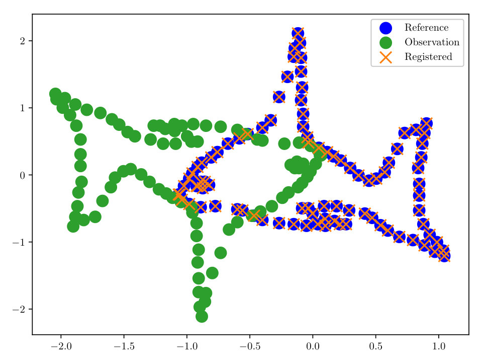 Figure 1
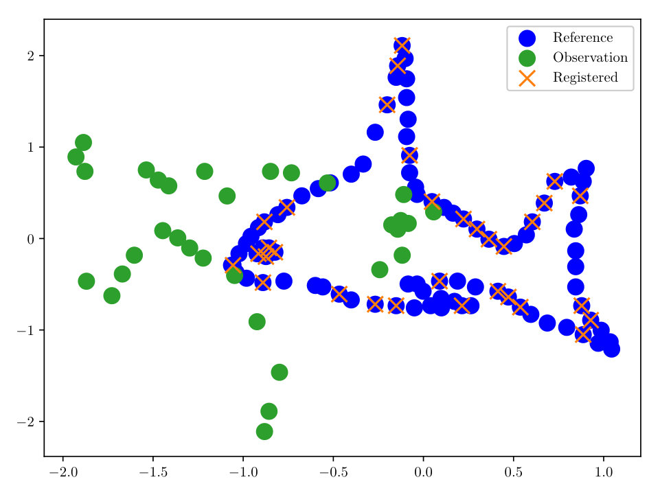 Figure 2
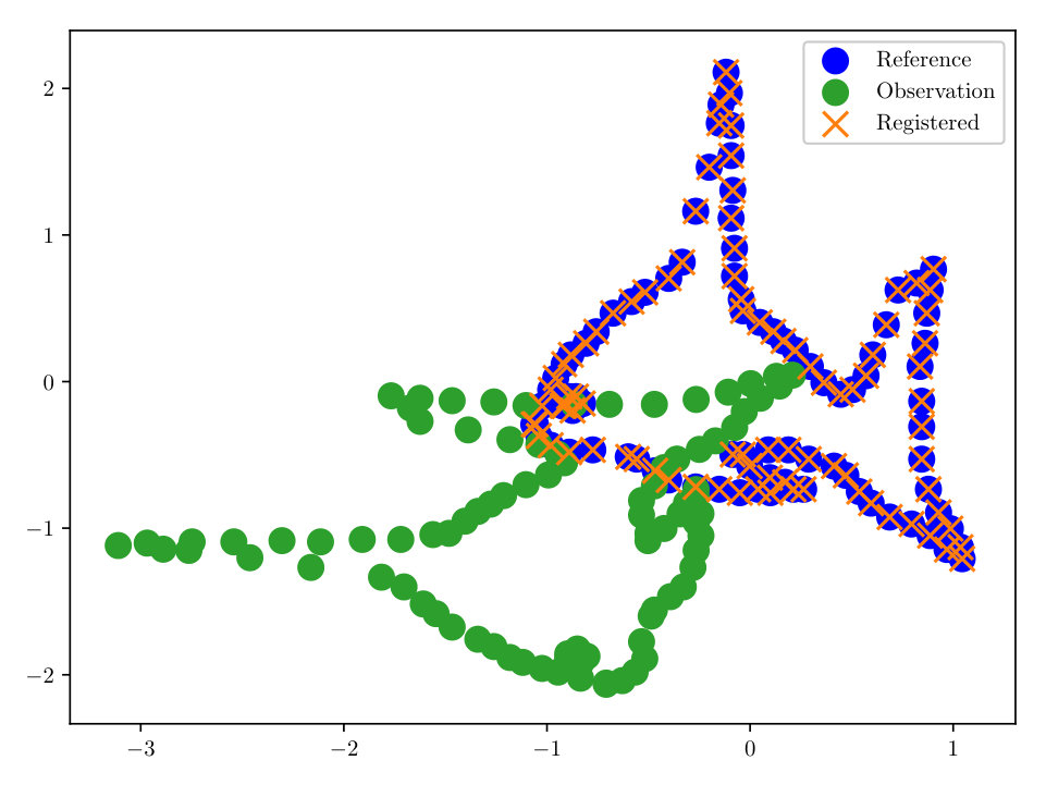 Figure 3
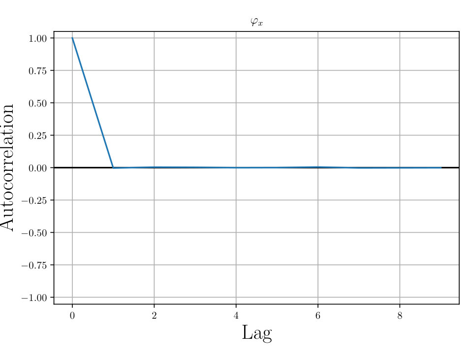 Figure 4
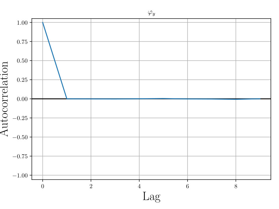 Figure 5
 Figure 6
 Figure 7
 Figure 8
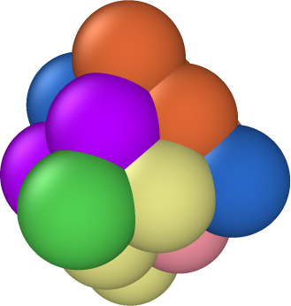 Figure 9
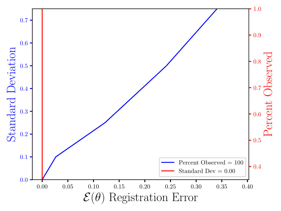 Figure 10
 Figure 11
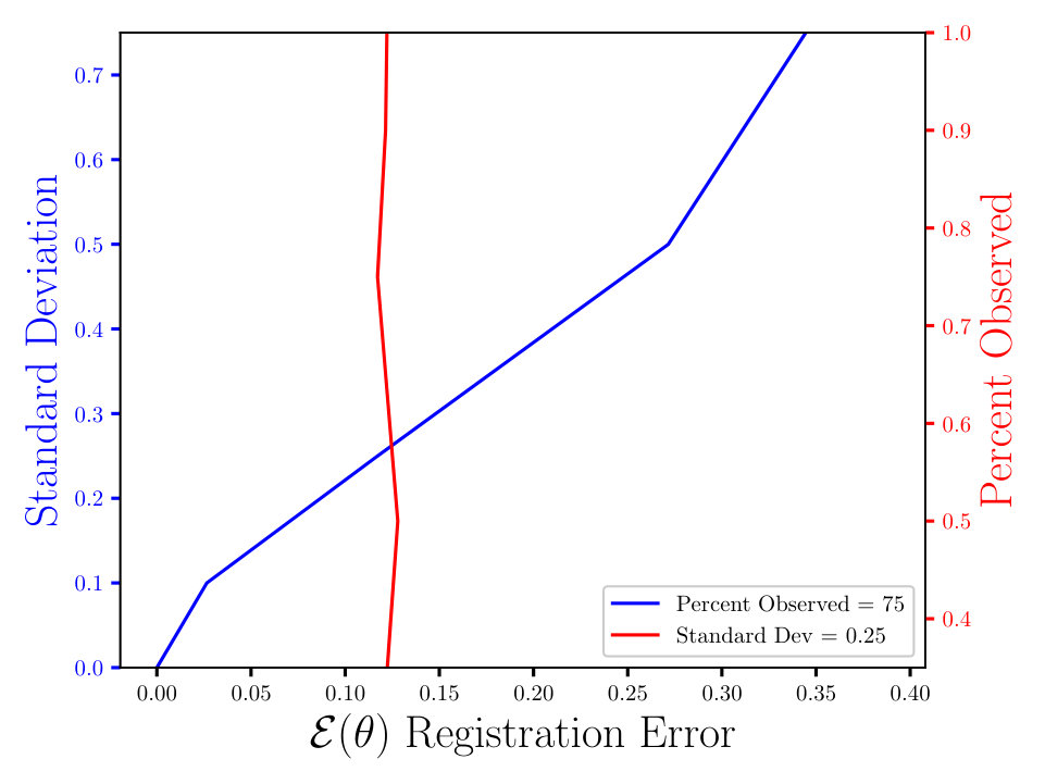 Figure 12
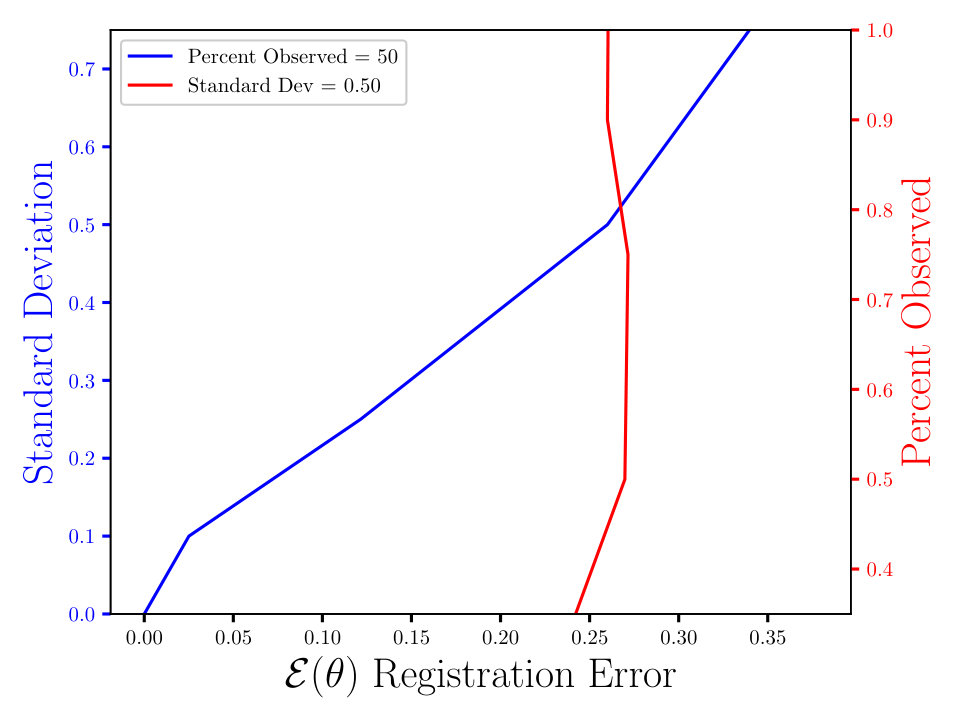 Figure 13
 Figure 14
 Figure 15
 Figure 16
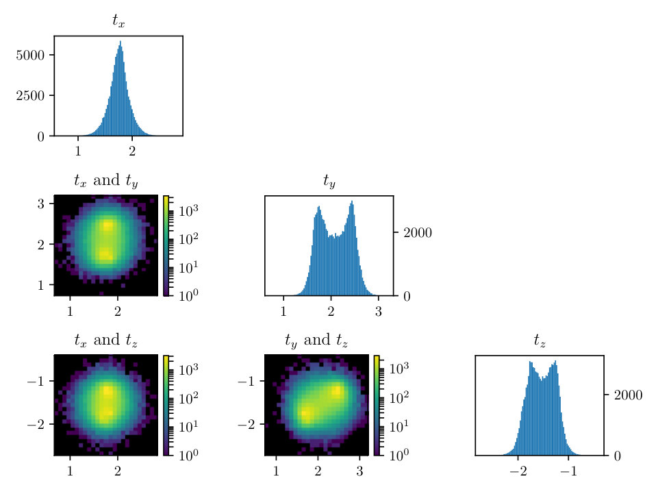 Figure 17
 Figure 18
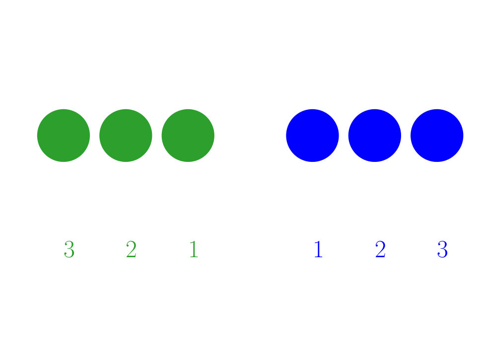 Figure 19
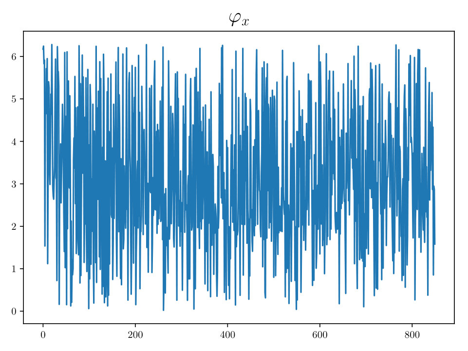 Figure 20
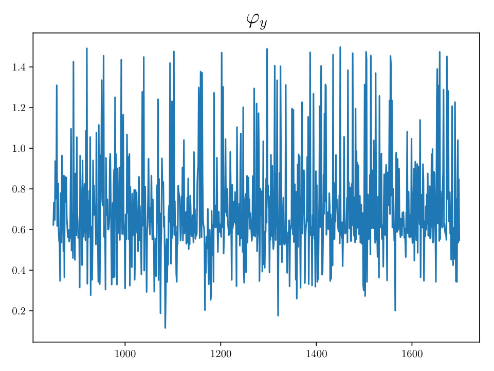 Figure 21
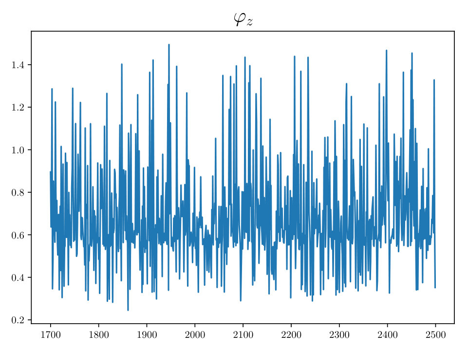 Figure 22
 Figure 23
 Figure 24
 Figure 25
 Figure 26
 Figure 27
 Figure 28
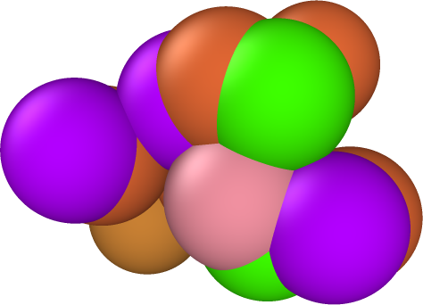 Figure 29
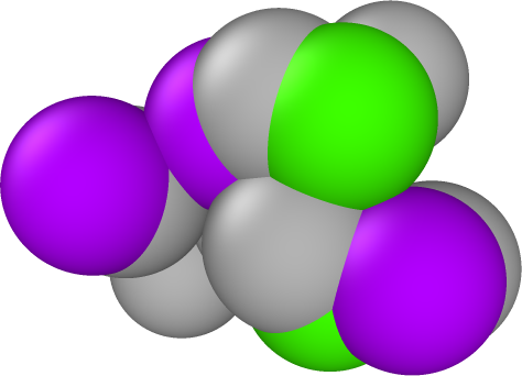 Figure 30
 Figure 31
 Figure 32
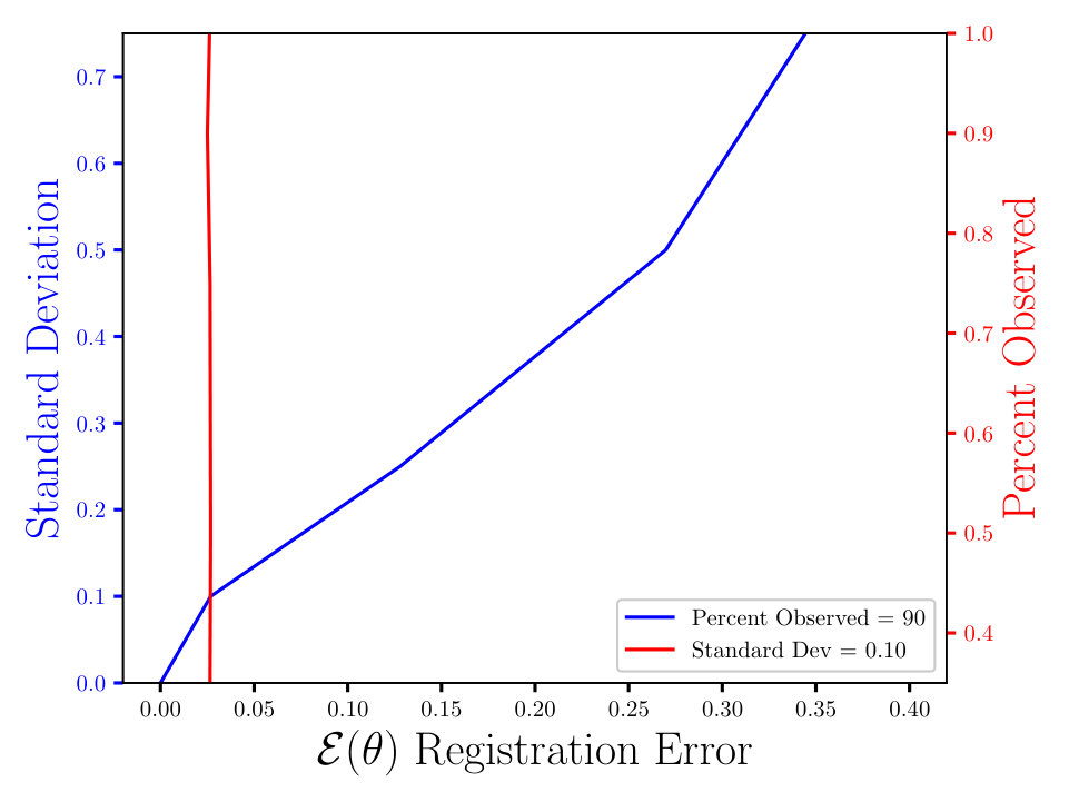 Figure 33
 Figure 34
 Figure 35
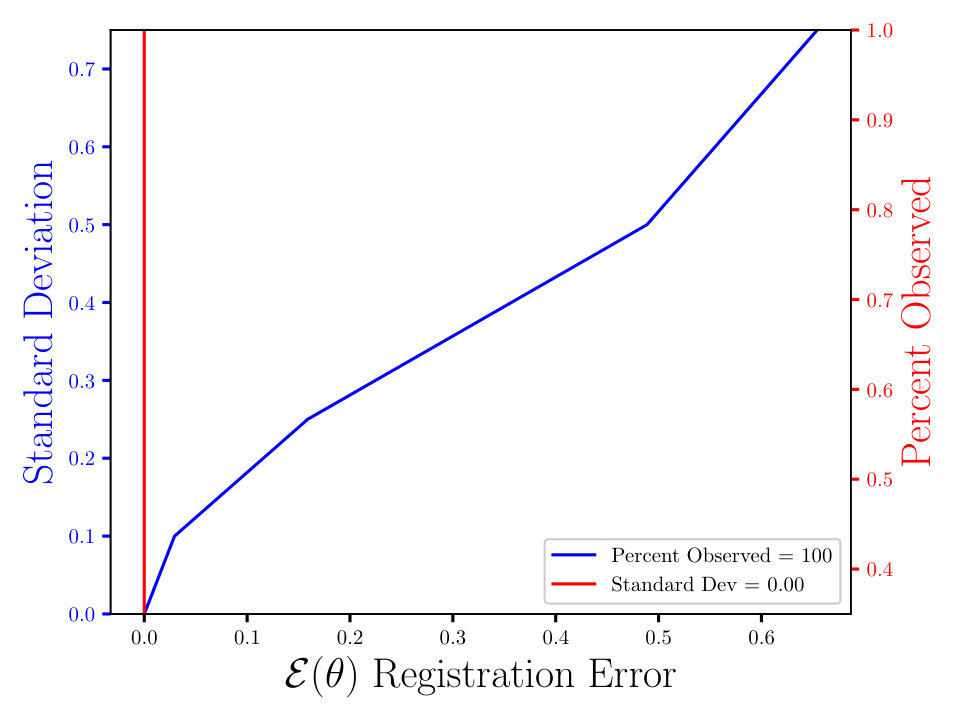 Figure 36
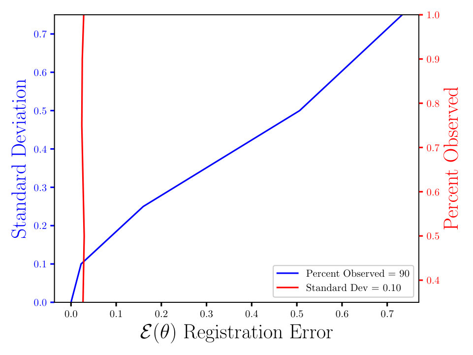 Figure 37
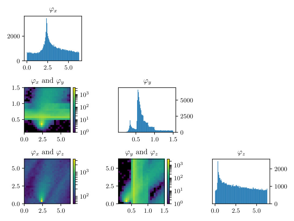 Figure 38
 Figure 39
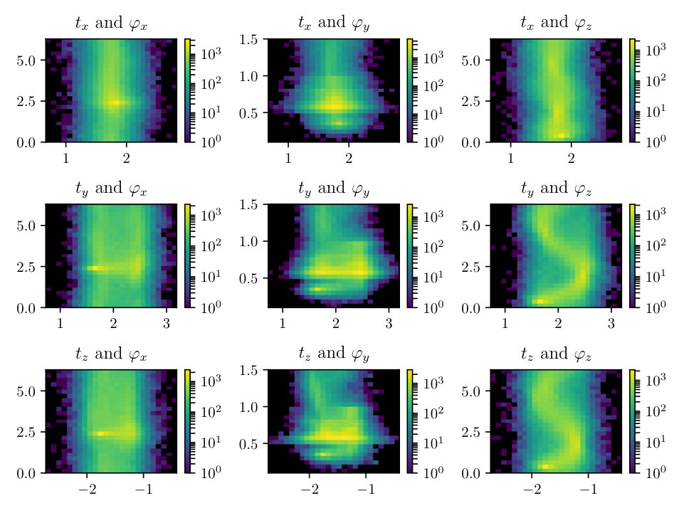 Figure 40
| Standard Deviation | Percent Observed | Registration Error |
|---|---|---|
| 0.0 | 75% | |
| 0.0 | 45% | |
| 0.25 | 75% | 0.1702529649951198 |
| 0.25 | 45% | 0.1221555853433331 |
| 0.5 | 75% | 0.3445684328735114 |
| 0.5 | 45% | 0.3643178111314804 |
| Standard Deviation | Percent Observed | Error |
|---|---|---|
| 0.25 | 75% | 0.04909611134835241 |
| 0.5 | 75% | 0.07934531875006196 |
| 0.25 | 45% | 0.07460005923988245 |
| 0.5 | 45% | 0.11978598998930728 |
Peer Reviews
No public reviews on file for this paper yet. If you reviewed it on a platform where reviews are public (OpenReview, ICLR, NeurIPS, ICML), you can paste yours below so the community can read it here.
Videos
No videos yet. Explain this paper in a talk, walkthrough, or lecture? Add one.
Taxonomy
TopicsArchaeology and ancient environmental studies · Geochemistry and Geologic Mapping · Cultural Heritage Materials Analysis
Bayesian Point Set Registration
Adam Spannaus
Department of Mathematics, University of Tennessee, Knoxville TN, USA 37996
,
Vasileios Maroulas
Department of Mathematics, University of Tennessee, Knoxville TN, USA 37996
,
David J. Keffer
Department of Materials Science and Engineering, University of Tennessee, Knoxville TN, USA 37996
and
Kody J. H. Law
School of Mathematics, University of Manchester, UK
Abstract.
Point set registration involves identifying a smooth invertible transformation between corresponding points in two point sets, one of which may be smaller than the other and possibly corrupted by observation noise. This problem is traditionally decomposed into two separate optimization problems: (i) assignment or correspondence, and (ii) identification of the optimal transformation between the ordered point sets. In this work, we propose an approach solving both problems simultaneously. In particular, a coherent Bayesian formulation of the problem results in a marginal posterior distribution on the transformation, which is explored within a Markov chain Monte Carlo scheme. Motivated by Atomic Probe Tomography (APT), in the context of structure inference for high entropy alloys (HEA), we focus on the registration of noisy sparse observations of rigid transformations of a known reference configuration. Lastly, we test our method on synthetic data sets.
Key words and phrases:
Point Set Registration, Bayesian Inference, MCMC, MALA
1. Introduction
In recent years, a new class of materials has emerged, called High Entropy Alloys (HEAs). The resulting HEAs possess unique mechanical properties and have shown marked resistance to high-temperature, corrosion, fracture and fatigue [5, 18]. HEAs demonstrate a ‘cocktail’ effect [7], in which the mixing of many components results in properties not possessed by any single component individually. Although these metals hold great promise for a wide variety of applications, the greatest impediment in tailoring the design of HEAs to specific applications is the inability to accurately predict their atomic structure and chemical ordering. This prevents Materials Science researchers from constructing structure-property relationships necessary for targeted materials discovery.
An important experimental characterization technique used to determine local structure of materials at the atomic level is Atomic Probe Tomography (APT) [8, 10]. APT provides an identification of the atom type and its position in space within the sample. APT has been successfully applied to the characterization of the HEA, AlCoCrCuFeNi [16]. Typically, APT data sets consist of to atoms. Sophisticated reconstruction techniques are employed to generate the coordinates based upon the construction of the experimental apparatus. APT data has two main drawbacks: (i) up to 66% of the data is missing and (ii) the recovered data is corrupted by noise. The challenge is to uncover the true atomic level structure and chemical ordering amid the noise and missing data, thus giving material scientists an unambiguous description of the atomic structure of these novel alloys. Ultimately, our goal is to infer the correct spatial alignment and chemical ordering of a dataset, herein referred to as a configuration, containing up to atoms. This configuration will be probed by individual registrations of the observed point sets in a neighborhood around each atom.
In this paper we outline our approach to this unique registration problem of finding the correct chemical ordering and atomic structure in a noisy and sparse dataset. While we do not solve the problem in full generality here, we present a Bayesian formulation of the model and a general algorithmic approach, which allows us to confront the problem with a known reference, and can be readily generalized to the full problem of an unknown reference.
In Section 2 we describe the problem and our Bayesian formulation of the statistical model. In Section 3, we describe Hamiltonian Monte Carlo, a sophisticated Markov chain Monte Carlo technique used to sample from multimodal densities, which we use in our numerical experiments in Section 4. Lastly, we conclude with a summary of the work presented here and directions for future research.
2. Problem Statement and Statistical Model
An alloy consists of a large configuration of atoms, henceforth “points”, which are rotated and translated instances of a reference collection of points, denoted for which is the matrix representation of the reference points. The tomographic observation of this configuration is missing some percentage of the points and is subject to noise, which is assumed additive and Gaussian. The sample consists of a single point and its nearest neighbors, where is of the order 10. If is the percent observed, i.e. means all points are observed and means no points are observed, then the reference point set will be comprised of points. We write the matrix representation of the noisy data point as , for .
The observed points have labels, but the reference points do not. We seek to register these noisy and sparse point sets, onto the reference point set. The ultimate goal is to identify the ordering of the labels of the points (types of atoms) in a configuration. We will find the best assignment and rigid transformation between the observed point set and the reference point set. Having completed the registration process for all observations in the configuration, we may then construct a three dimensional distribution of labeled points around each reference point, and the distribution of atomic composition is readily obtained.
The point-set registration problem has two crucial elements. The first is the correspondence, or assignment of each point in the observed set to the reference set. The second is the identification of the optimal transformation from within an appropriate class of transformations. If the transformation class is taken to be the rigid transformations, then each of the individual problems is easily solved by itself, and naive methods simply alternate the solution of each individually until convergence.
One of the most frequently used point set registration algorithms is the iterative closest point method, which alternates between identifying the optimal transformation for a given correspondence, and then corresponding closest points [1]. If the transformation is rigid, then both problems are uniquely solvable. If instead we replace the naive closest point strategy with the assignment problem, so that any two observed points correspond to two different reference points, then again the problem can solved with a linear program [9]. However, when these two solvable problems are combined into one, the resulting problem is non-convex [14], and no longer admits a unique solution, even for the case of rigid transformations as considered here. The same strategy has been proposed with more general non-rigid transformations [3], where identification of the optimal transformation is no longer analytically solvable. The method in [11] minimizes an upper bound on their objective function, and is thus also susceptible to getting stuck in a local basin of attraction. We instead take a Bayesian formulation of the problem that will simultaneously find the transformation and correspondence between point sets. Most importantly, it is designed to avoid local basins of attraction and locate a global minimum.
We will show how alternating between finding correspondences and minimizing distances can lead to an incorrect registration. Consider now the setup in Fig. (1). If we correspond closest points first, then all three green points would be assigned to the blue ‘1’. Then, identifying the single rigid transformation to minimize the distances between all three green and the blue ‘1’ would yield a local minimum, with no correct assignments. If we consider instead assignments, so that no two observation points can correspond to the same reference point, then again it is easy then to see two equivalent solutions with the eye. The first is a pure translation, and the second can be obtained for example by one of two equivalent rotations around the mid-point between ‘1’s, by or . The first only gets the assignment of ‘2’ correct, while the second is correct. Note that in reality the reference labels are unknown, so both are equivalent for us.
Here it is clear what the solutions are, but once the problem grows in scale, the answer is not always so clear. This simple illustration of degenerate (equal energy) multi-modality of the registration objective function arises from physical symmetry of the reference point-set. This will be an important consideration for our reference point sets, which will arise as a unit cell of a lattice, hence with appropriate symmetry. We will never be able to know the registration beyond these symmetries, but this will nonetheless not be the cause of concern, as symmetric solutions will be considered equivalent. The troublesome multi-modality arises in the presence of noisy and partially observed point sets, where there may be local minima with higher energy than the global minima.
The multi-modality of the combined problem, in addition to the limited information in the noisy and sparse observations, motivates the need for a global probabilistic notion of solution for this problem. It is illustrated in the following subsection that the problem lends itself naturally to a flexible Bayesian formulation which circumvents the intrinsic shortcomings of deterministic optimization approaches for non-convex problems. Indeed at an additional computational cost, we obtain a distribution of solutions, rather than a point estimate, so that general quantities of interest are estimated and uncertainty is quantified. In case a single point estimate is required we define an appropriate optimal one (for example the global energy minimizer or probability maximizer).
2.1. Bayesian Formulation
We seek to compute the registration between the observation set and reference set. We are concerned primarily with rigid transformations of the form
[TABLE]
where is a rotation and is a translation vector.
Write for , , and where is the ith column of . Now let with entries , and assume the following statistical model
[TABLE]
for and independent.
The matrix of correspondences , is such that , and each observation point corresponds to only one reference point. So if matches then , otherwise, . We let be endowed with a prior, for and . Furthermore, assume a prior on the transformation parameter given by . The posterior distribution then takes the form
[TABLE]
where is the likelihood function associated with Eqn. (1).
For a given , an estimate can be constructed a posteriori by letting for and zero otherwise, where
[TABLE]
For example, may be taken as the maximum a posteriori (MAP) estimator or the mean. We note that can be constructed either with a closest point approach, or via assignment to avoid multiple registered points assigned to the same reference.
Lastly, we assume the observation only depends on the column of the correspondence matrix, and so are conditionally independent with respect to the matrix for . This does not exclude the case where multiple observation points are assigned to the same reference point, but as mentioned above such scenario should have zero probability.
To that end, instead of considering the full joint posterior in Eqn. (3) we will focus on the marginal of the transformation
[TABLE]
Let denote the column of . Since is completely determined by the single index at which it takes the value 1, the marginal likelihood takes the form
[TABLE]
The above marginal together with the conditional independence assumption allows us to construct the likelihood function of the marginal posterior, Eqn. (5), as follows
[TABLE]
Thus the posterior in question is
[TABLE]
At its heart, point set registration is an optimization problem. Consider a prior on such that , where . Then we have the following objective function
[TABLE]
The minimizer, , of the above, Eqn. (9) is also the maximizer of a posteriori probability under Eqn. (2.1). It is called the maximum a posteriori estimator. This can also be viewed as maximum likelihood estimation regularized by .
By sampling consistently from the posterior, we may estimate quantities of interest, such as moments, together with quantified uncertainty. Additionally, we may recover other point estimators, such as local and global modes.
3. Hamiltonian Monte Carlo
Monte Carlo Markov chain (MCMC) methods are a natural choice for sampling from distributions which can be evaluated pointwise up to a normalizing constant, such as the posterior Eqn. (2.1). Furthermore, MCMC comprises the workhorse of Bayesian computation, often appearing as crucial components of more sophisticated sampling algorithms. Formally, an MCMC simulates a distribution over a state space by producing an ergodic Markov chain that has as its invariant distribution, i.e.
[TABLE]
with probability 1, for .
The Metropolis-Hastings method is a general MCMC method defined by choosing and iterating the following two steps for
- (1)
Propose: .
- (2)
Accept/reject: Let with probability
[TABLE]
and otherwise.
In general, random-walk proposals can result in MCMC chains which are slow to explore the state space and susceptible to getting stuck in local basins of attraction. Hamiltonian Monte Carlo (HMC) is designed to improve this shortcoming. HMC is a Metropolis-Hastings method [4, 13] which incorporates gradient information of the log density with a simulation of Hamiltonian dynamics to efficiently explore the state space and accept large moves of the Markov chain. Heuristically, the gradient yields pieces of information, for a -valued variable and scalar objective function, as compared with one piece of information from the objective function alone. Our description here of the HMC algorithm follows that of [2] and the necessary foundations of Hamiltonian dynamics for the method can be found in [17].
Our objective here is to sample from a specific target density
[TABLE]
over , where is as defined in Eqn. (9) and is of the form given by Eqn. (2.1).
First, an artificial momentum variable , independent of , is included into Eqn. (11), for a symmetric positive definite mass matrix , that is usually a scalar multiple of the identity matrix. Define a Hamiltonian now by
[TABLE]
where is the “potential energy” and is the “kinetic energy”.
Hamilton’s equations of motion for are, for :
[TABLE]
In practice, the algorithm creates a Markov chain on the joint position-momentum space , by alternating between independently sampling from the marginal Gaussian on momentum , and numerical integration of Hamiltonian dynamics along an energy contour to update the position. If the initial condition and we were able to perfectly simulate the dynamics, this would give samples from because the Hamiltonian remains constant along trajectories. Due to errors in numerical approximation, the value of will vary. To ensure the samples are indeed drawn from the correct distribution, a Metropolis-Hastings accept/reject step is incorporated into the method.
In particular, after a new momentum is sampled, suppose the chain is in the state . Provided the numerical integrator is reversible, the probability of accepting the proposed point takes the form
[TABLE]
If is rejected, the next state remains unchanged from the previous iteration. However, note that a fresh momentum variable is drawn each step, so only remains fixed. Indeed the momentum variables can be discarded, as they are only auxiliary variables. To be concrete, the algorithm requires an initial state , a reversible numerical integrator, integration step-size , and number of steps . Note that reversibility of the integrator is crucial such that the proposal integration is symmetric and drops out of the acceptance probability in Eqn. (12). The parameters and are tuning parameters, and are described in detail [2, 13].
The HMC algorithm then proceeds as follows:
for do HMC:
for
function Integrator() return
end function
with probability ** otherwise**
end for
Under appropriate assumptions [13], this method will provide samples , such that for bounded
[TABLE]
4. Numerical Experiments
To illustrate our approach, we consider numerical experiments on synthetic datasets in and , with varying levels of noise and percentage of observed data. We focus our attention to rigid transformations of the form Eqn. (1).
For all examples here, the observation points are simulated as , for a rotation matrix parameterized by , and some and . So, . To simulate the unknown correspondence between the reference and observation points, for each , the corresponding index is chosen randomly and without replacement. Recall that we define percentage of observed points here as .We tested various percentages of observed data and noise on the observation set, then computed the mean square error (MSE), given by Eqn. (13), between the reference points and the registered observed points,
[TABLE]
4.1. Two Dimensional Registration
First we consider noise-free data, i.e. (however in the reconstruction some small is used). The completed registration for the 2-dimensional ‘fish’ set is shown in Figs. (3, 3). The ‘fish’ set is a standard benchmark test case for registration algorithms in [6, 12]. Our methodology, employing the HMC sampler described in Sect. 3 allows for a correct registration, even in the case where we have only 33% of the initial data, see Fig. (3).
As a final experiment with the ‘fish’ dataset, we took 25 independent identically distributed (i.i.d.) realizations of the reference, all having the same transformation, noise, and percent observed. Since we have formulated the solution of our registration problem as a density, we may compute moments, and find other quantities of interest. In this experiment we evaluate , where is our MAP estimator of from the HMC algorithm. We then evaluated the transformation under . The completed registration is shown in Fig. (4). With a relatively small number of configurations, we are able to accurately reconstruct the data, despite the noisy observations.
4.2. Synthetic APT Data
The datasets from APT experiments are perturbed by additive noise on each of the points. The variance of this additive noise is not known in general, and so in practice it should be taken as a hyper-parameter, endowed with a hyper-prior, and inferred or optimized. It is known that the size of the displacement on the order of several Å (Angstroms), so that provides a good basis for choice of hyper prior. In order to simulate this uncertainty in our experiments, we incorporated additive noise in the form of a truncated Gaussian, to keep all the mass within several Å . The experiments consider a range of variances in order to measure the impact of noise on our registration process.
In our initial experiments with synthetic data, we have chosen percentages of observed data and additive noise similar to what Materials Scientist experimentalists have reported in their APT datasets. The percent observed of these experimental datasets is approximately 33%. The added noise of these APT datasets is harder to quantify. Empirically, we expect the noise to be Gaussian in form, truncated to be within 1-3 Å. The standard deviation of the added noise is less well-known, so we will work with different values to asses the method’s performance. With respect to the size of the cell, a displacement of 3Å is significant. Consider the cell representing the hidden truth in Fig. (5). The distance between the front left and right corners is on the scale of 3Å. Consequently a standard deviation of 0.5 for the additive noise represents a significant displacement of the atoms.
As a visual example, the images in Fig. (5) are our synthetic test data used to simulate the noise and missing data from the APT datasets. The leftmost image in Fig. (5) is the hidden truth we seek to uncover. The middle image is the first with noise added to the atom positions. Lastly, in the right-most image we have ‘ghosted’ some atoms, by coloring them grey, to give a better visual representation of the missing data. In these representations of HEAs, a color different from grey denotes a distinct type of atom. What we seek is to infer the chemical ordering and atomic structure of the left image, from transformed versions of the right, where .
For our initial numerical experiments with simulated APT data, we choose a single reference and observation, and consider two different percentages of observed data, 75% and 45%. For both levels of observations in the data, we looked at results with three different levels of added noise on the atomic positions: no noise, and Gaussian noise with standard deviation of 0.25 and 0.5. The MSE of the processes are shown in Table 1. We initially observe the method is able, within an appreciably small tolerance, find the exact parameter in the case of no noise, with both percentages of observed data. In the other cases, as expected, the error scales with the noise. This follows from our model, as we are considering a rigid transformation between the observation and reference, which is a volume preserving transformation. If the exact transformation is used with an infinite number of points, then the RMSE (square root of Eqn. (13)) is .
Now we make the simplifying assumption that the entire configuration corresponds to the same reference, and each observation in the configuration corresponds to the same transformation applied to the reference, with i.i.d. noise added to it. This enables us to approximate the mean and variance of Eqn. (13) over these observation realizations, i.e. we obtain a collection of errors, where is the MSE corresponding to replacing and its estimated registration parameters into Eqn. (13), where is the total number of completed registrations. The statistics of this collection of values provide robust estimates of the expected error for a single such registration, and the variance we can expect over realizations of the observational noise. In other words
[TABLE]
We have confidence intervals as well, corresponding to a central limit theorem approximation based on these samples.
In Figs. (7 - 9) we computed the registration for i.i.d. observation sets corresponding to the same reference, for each combination of noise and percent observed data. We then averaged all 125 registration errors for a fixed noise/percent observed combination, as in Eqn. (14), and compared the values. What we observe in Figs. (7 - 9) is the registration error scaling with the noise, which is expected. What is interesting to note here is that the registration error is essentially constant with respect to the percentage of observed data, for a fixed standard deviation of the noise. More information will lead to a lower variance in the posterior on the transformation , following from standard statistical intuition. However, the important point to note is that, as mentioned above, for exact transformation, and infinite points, Eqn. (13) will equal . So, for sufficiently accurate transformation, one can expect a sample approximation thereof. Sufficient accuracy is found here with very few observed points, which is reasonable considering that in the zero noise case 2 points is sufficient to fit the 6 parameters exactly.
The MSE registration errors shown in Figs. (7 - 9), show the error remains essentially constant with respect to the percent observed. Consequently, if we consider only Fig. (7), we observe that the blue and red lines intersect, when the blue has a standard deviation of 0.1, and the associated MSE is approximately 0.05. This same error estimate holds for all tested percentages of observed data having a standard deviation of 0.1. Similar results hold for other combinations of noise and percent observed, when the noise is fixed.
Furthermore, the results shown in Figs. (7 - 9) are independent of the algorithm, as the plots in Figs. (11 - 11) show. For the latter, we ran a similar experiment with 125 i.i.d. observation sets, but to compute the registration, we used the Metropolis Adjusted Langevin Algorithm (MALA) [15], as opposed to HMC in Figs. (7 - 9). Both algorithms solve the same problem and use information from the gradient of the log density. In the plots shown in Figs. (7 - 9), we see the same constant error with respect to the percent observed and the error increasing with the noise, for a fixed percent observed. The MSE also appears to be proportional to , which is expected, until some saturation threshold of or so. This can be understood as a threshold beyond which the observed points will tend to get assigned to the wrong reference point.
To examine the contours of our posterior described by Eqn. (2.1), we drew samples from the density using the HMC methodology described previously. For this simulation we set the noise to have standard deviation of 0.25 and the percent observed was 35%, similar values to what we expect from real APT datasets. The rotation matrix is constructed via Euler angles denoted: , where and These parameters are especially important to making the correct atomic identification, which is crucial to the success of our method.
In Figs. (12 - 14), we present marginal single variable histograms and all combinations of marginal two-variable joint histograms for the individual components of . We observe multiple modes in a number of the marginals. In Figs. (15 - 20) we present autocorrelation and trace plots for the rotation parameters from the same instance of the HMC algorithm as presented in the histograms above in Figs. (12 - 14). We focus specifically on the rotation angles, to ensure efficient mixing of the Markov chain as these have thus far been more difficult for the algorithm to optimize. We see the chain is mixing well with respect to these parameters and appears not to become stuck in local basins of attraction.
Additionally, we consider the following. Define null sets . For each and , let , and increment . This provides a distribution of registered points for each index , , from which we estimate various statistics such as mean and variance. However, note that the cardinality varies between . We are only be concerned with statistics around reference points such that or so, assuming that the other reference points correspond to outliers which were registered to by accident. Around each of these reference points , we have a distribution of some registered points. We then computed the mean of these points, denoted by and finally we compute the MSE . The RMSE is reported in Table 2. Here we note that a lower percentage observed is correlated with a larger error. Coupling correct inferences about spatial alignment with an ability to find distributions of atoms around each lattice point is a transformative tool for understanding High Entropy Alloys.
5. Conclusion
We have presented a statistical model and methodology for point set registration. We are able to recover a good estimate of the correspondence and spatial alignment between point sets in and despite missing data and added noise. As a continuation of this work, we will extend the Bayesian framework presented in section to incorporate the case of an unknown reference. In such a setting, we will seek not only the correct spatial alignment and correspondence, but the reference point set, or crystal structure. The efficiency of our algorithm could be improved through a tempering scheme, allowing for easier transitions between modes, or an adaptive HMC scheme, where the chain learns about the sample space in order to make more efficient moves.
Being able to recover the alignment and correspondences with an unknown reference will give Materials Science researchers an unprecedented tool in making accurate predictions about High Entropy Alloys and allow them to develop the necessary tools for classical interaction potentials. Researchers working in the field will be able to determine the atomic level structure and chemical ordering of High Entropy Alloys. From such information, the Material Scientists will have the necessary tools to develop interaction potentials, which is crucial for molecular dynamics simulations and designing these complex materials.
Acknowledgments
A.S. would like to thank ORISE as well as Oak Ridge National Laboratory (ORNL) Directed Research and Development funding. In addition, he thanks the CAM group at ORNL for their hospitality. K.J.H.L. gratefully acknowledges the support of Oak Ridge National Laboratory Directed Research and Development funding.
The reference list from the paper itself. Each links out to its DOI / PubMed record.
- 1[1] P. J. Besl and N. D. Mc Kay , A method for registration of 3-d shapes , IEEE Transactions on Pattern Analysis and Machine Intelligence, 14 (1992), pp. 239–256.
- 2[2] S. Brooks, A. Gelman, G. Jones, and X.-L. Meng , Handbook of markov chain monte carlo , CRC press, 2011.
- 3[3] H. Chui and A. Rangarajan , A new point matching algorithm for non-rigid registration , Computer Vision and Image Understanding, 89 (2003), pp. 114–141.
- 4[4] S. Duane, A. D. Kennedy, B. J. Pendleton, and D. Roweth , Hybrid monte carlo , Physics letters B, 195 (1987), pp. 216–222.
- 5[5] M. C. Gao, J.-W. Yeh, P. K. Liaw, and Y. Zhang , High-entropy alloys: fundamentals and applications , Springer, 2016.
- 6[6] B. Jian and B. C. Vemuri , Robust point set registration using gaussian mixture models , IEEE Transactions on Pattern Analysis and Machine Intelligence, 33 (2011), pp. 1633–1645.
- 7[7] Y. Jien-Wei , Recent progress in high entropy alloys , Ann. Chim. Sci. Mat, 31 (2006), pp. 633–648.
- 8[8] D. Larson, T. Prosa, R. Ulfig, B. Geiser, and T. Kelly , Local Electrode Atom Probe Tomography: A User’s Guide , Springer, 2013.