Quantum Information Geometry in the Space of Measurements
Warner A. Miller

TL;DR
This paper introduces a novel information geometry approach to analyze entangled quantum networks by examining measurement data, providing new insights into quantum state characterization and potential scalability benefits.
Contribution
It extends information geometry methods from bipartite to tripartite quantum states using measurement outcome data, offering a new way to characterize complex quantum networks.
Findings
Applied to GHZ, W, and separable states, demonstrating the method's effectiveness.
Generalized geometric measures to higher dimensions like area and volume.
Potential for improved scalability in quantum state analysis.
Abstract
We introduce a new approach to evaluating entangled quantum networks using information geometry. Quantum computing is powerful because of the enhanced correlations from quantum entanglement. For example, larger entangled networks can enhance quantum key distribution (QKD). Each network we examine is an n-photon quantum state with a degree of entanglement. We analyze such a state within the space of measured data from repeated experiments made by n observers over a set of identically-prepared quantum states -- a quantum state interrogation in the space of measurements. Each observer records a 1 if their detector triggers, otherwise they record a 0. This generates a string of 1's and 0's at each detector, and each observer can define a binary random variable from this sequence. We use a well-known information geometry-based measure of distance that applies to these binary strings of…
Click any figure to enlarge with its caption.
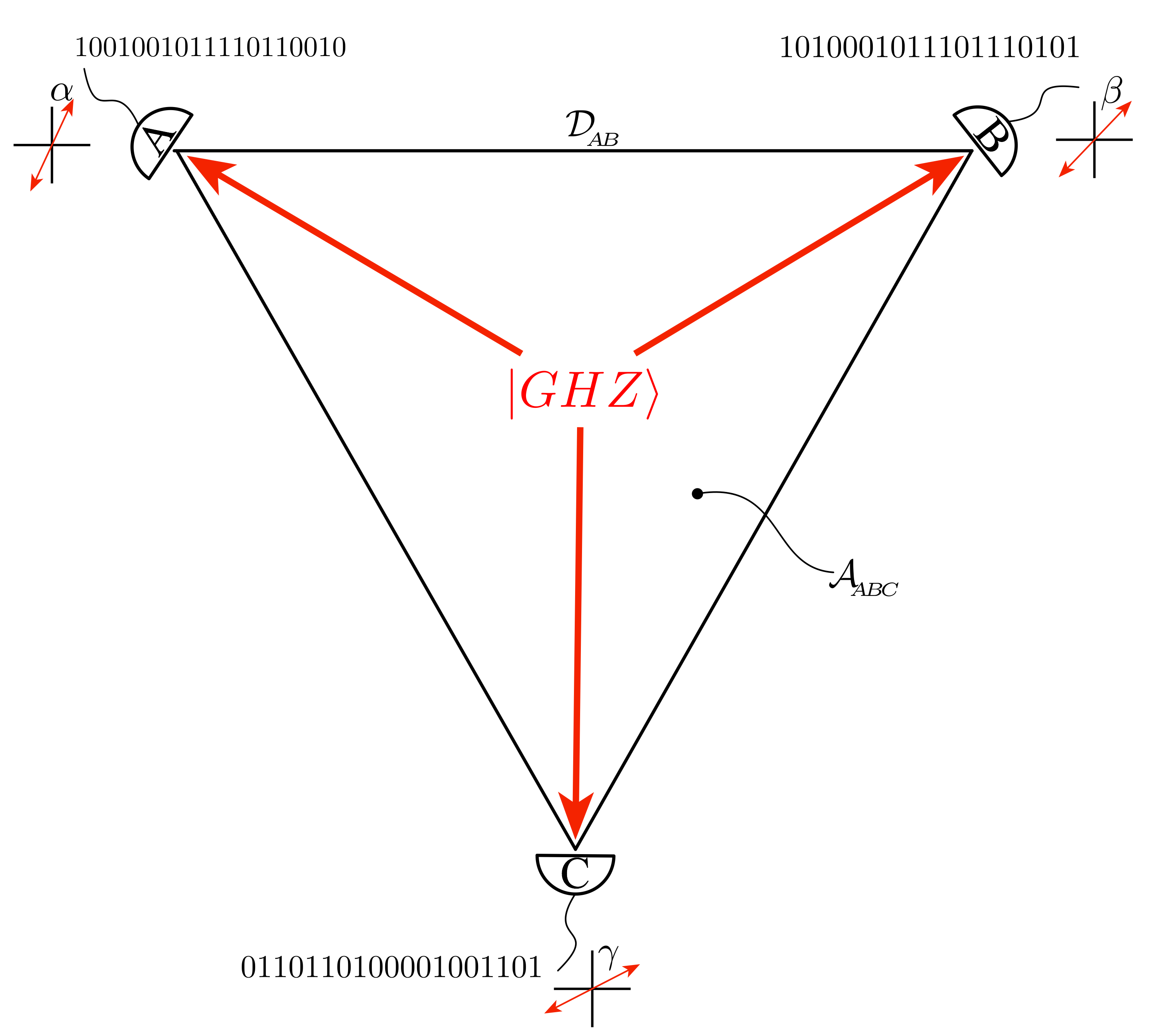 Figure 1
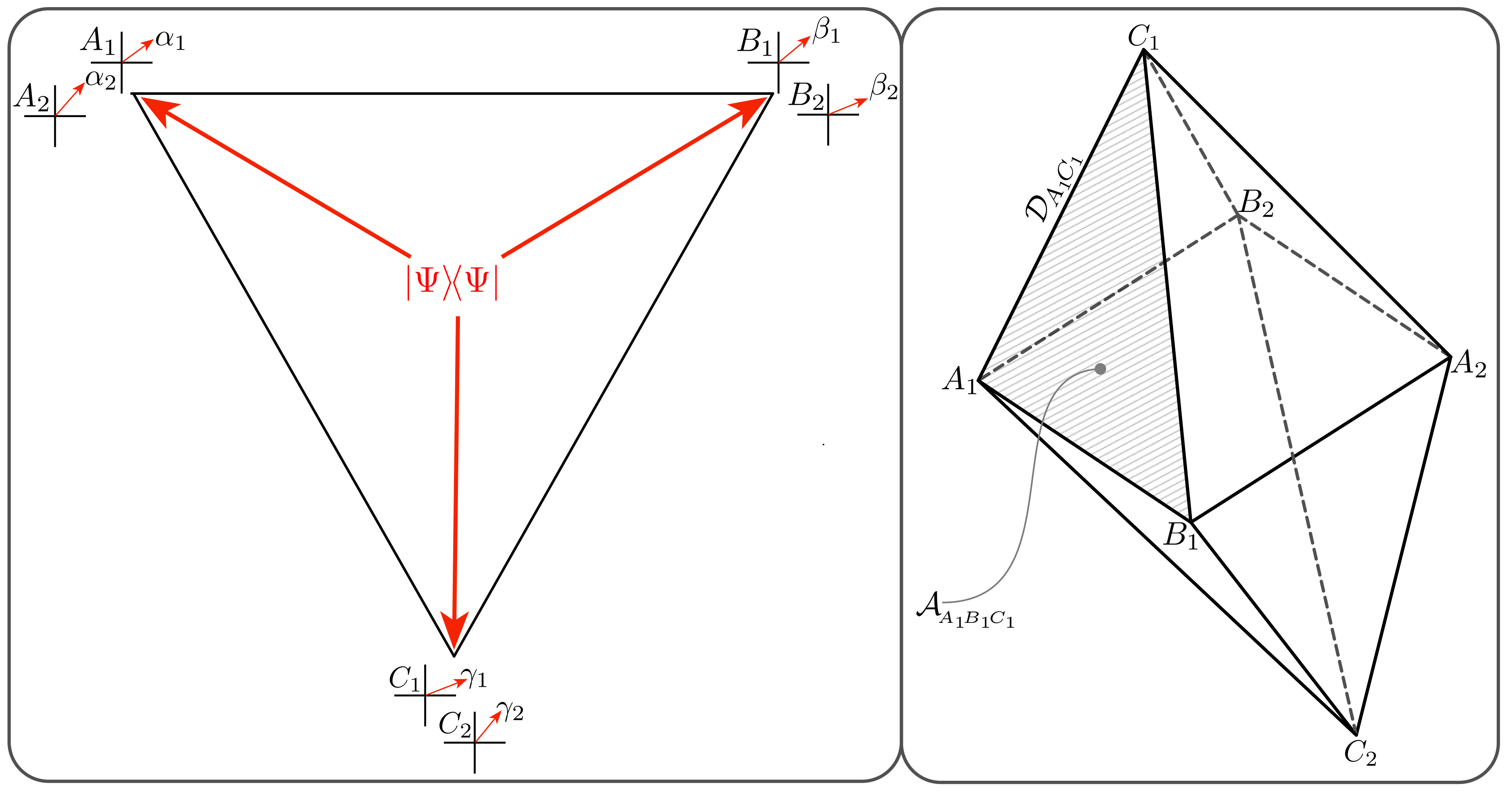 Figure 2
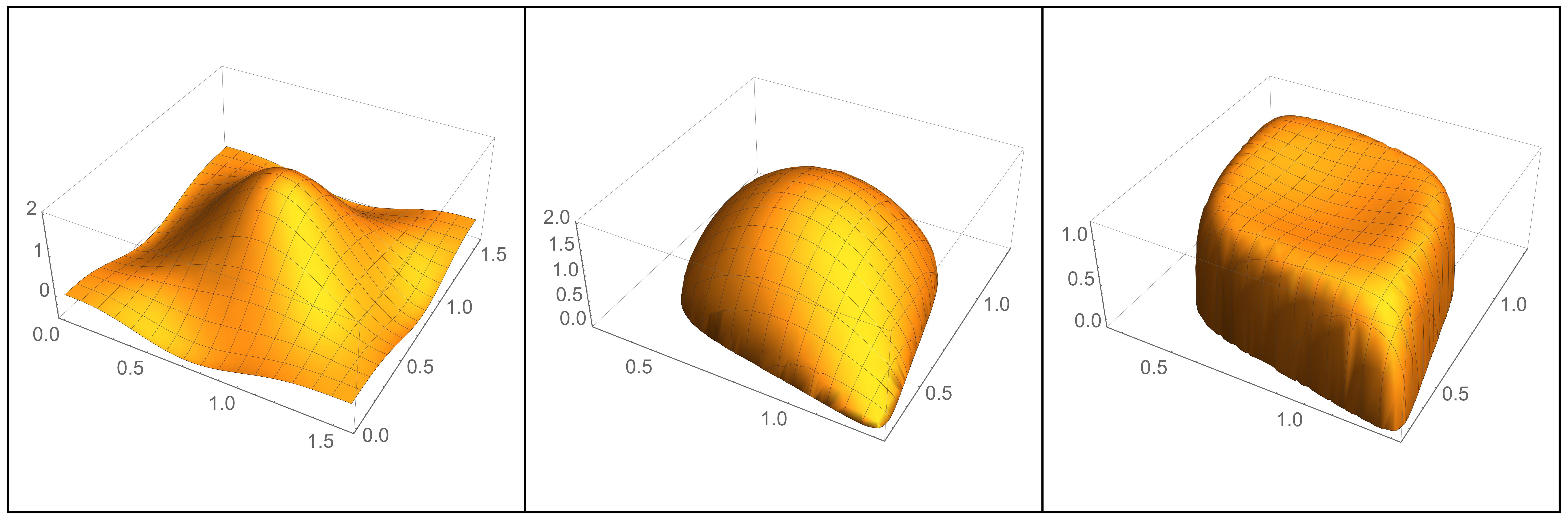 Figure 3
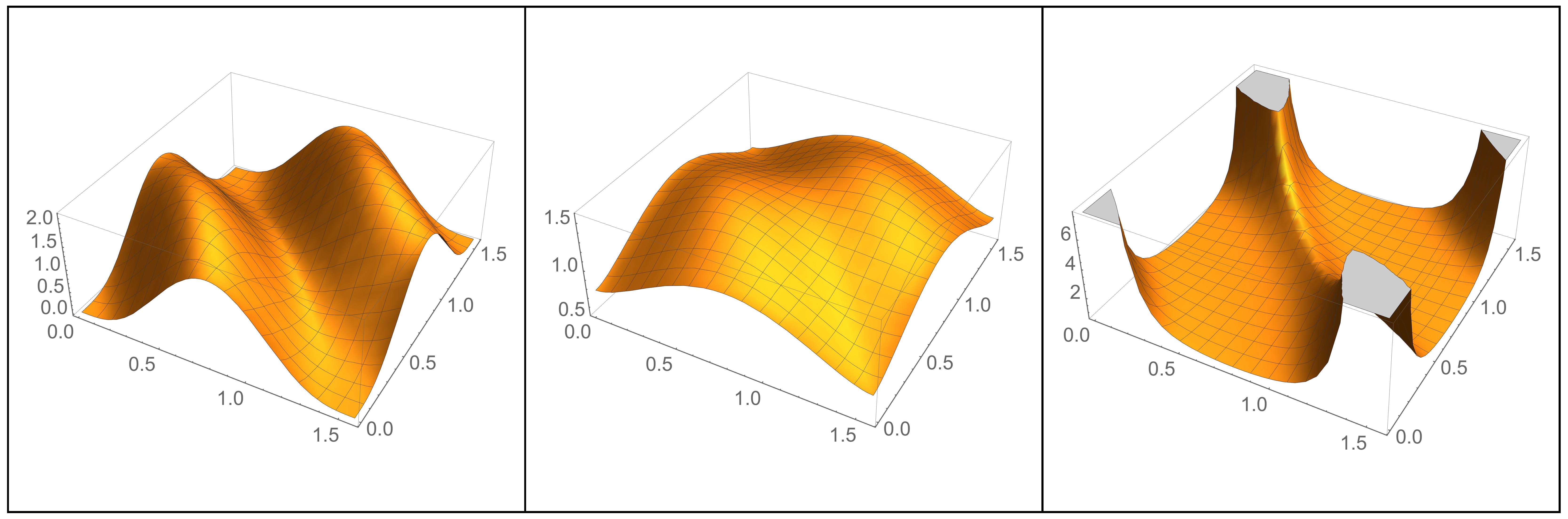 Figure 4
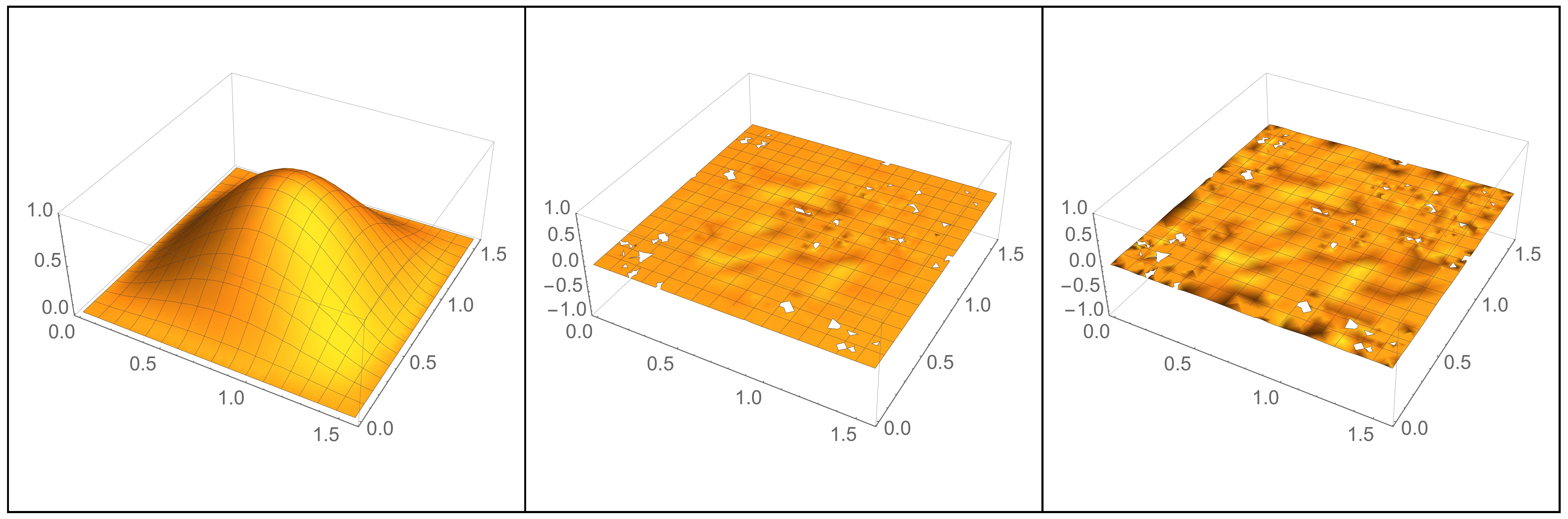 Figure 5
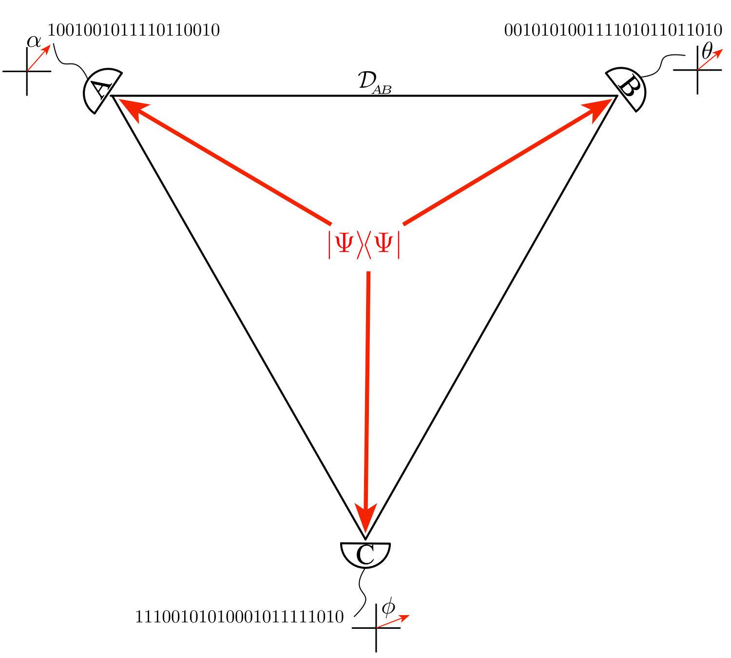 Figure 6
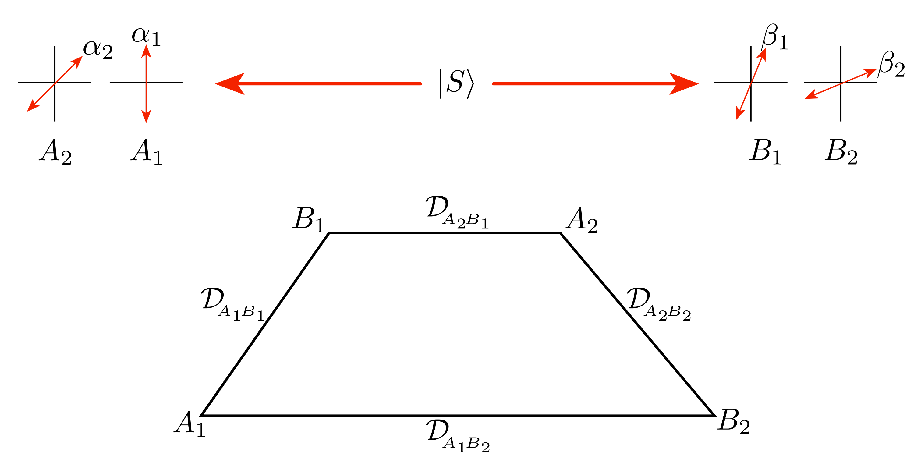 Figure 7
Peer Reviews
No public reviews on file for this paper yet. If you reviewed it on a platform where reviews are public (OpenReview, ICLR, NeurIPS, ICML), you can paste yours below so the community can read it here.
Videos
No videos yet. Explain this paper in a talk, walkthrough, or lecture? Add one.
Quantum Information Geometry in the
Space of Measurements
Warner A. Miller
Department of Physics, Florida Atlantic University, Boca Raton, FL, 33431
Abstract.
We introduce a new approach to evaluating entangled quantum networks using information geometry. Quantum computing is powerful because of the enhanced correlations from quantum entanglement. For example, larger entangled networks can enhance quantum key distribution (QKD). Each network we examine is an -photon quantum state with a degree of entanglement. We analyze such a state within the space of measured data from repeated experiments made by observers over a set of identically-prepared quantum states – a quantum state interrogation in the space of measurements. Each observer records a if their detector triggers, otherwise they record a [math]. This generates a string of ’s and [math]’s at each detector, and each observer can define a binary random variable from this sequence. We use a well-known information geometry-based measure of distance that applies to these binary strings of measurement outcomes [9, 7, 14], and we introduce a generalization of this length to area, volume and higher-dimensional volumes [2]. These geometric equations are defined using the familiar Shannon expression for joint and mutual entropy [11]. We apply our approach to three distinct tripartite quantum states: the state, the state, and a separable state . We generalize a well-known information geometry analysis of a bipartite state to a tripartite state. This approach provides a novel way to characterize quantum states, and it may have favorable scaling with increased number of photons.
1. INTRODUCTION
“No elementary quantum phenomenon is a phenomenon until it is brought to close by an irreversible act of amplification.” This Niels Bohr-inspired quantum adage of John Archibald Wheeler, together with the Principle of Complementarity, is at the very heart of Wheeler’s It-from-Bit framework [13]. In this manuscript, we explore entanglement networks within this information-centric approach. The quantum network we consider in this manuscript is a quantum state with photons with varying degrees of entanglement. Observers examine the space of measured data from repeated experiments on a set of identically-prepared quantum states. Each observer records a if their detector triggers, otherwise a ”0” is recorded. This generates a string of ’s and [math]’s at each detector as illustrated in Fig. 1. The string of numbers can be represented by a binary random variable. The observers may have more than one detector, and therefore each observer may acquire more than one binary random variable. Once these random variables are formed, we can apply an information geometry measure of distance, area, volume and n-volumes to the network of observers [9, 7, 2, 14]. These measures are defined using the familiar Shannon expression for mutual and conditional entropy [11]. This will be discussed in Sec. 2. In Sec. 4, we apply our approach to three distinct tripartite quantum states: the state, the state, and a separable state . This novel approach provides us with a natural generalization an information geometry model of Bell’s inequality for a bipartite singlet state to a similar analysis tripartite states [10]. We provide a brief review of this 2-photon geometry in Sec. 3 and its generalization in Sec. 5.
The power of quantum computing stems from a network of quantum entanglement, and larger networks can enhance quantum key distribution (QKD)[5, 6, 8]. Consequently, a primary focus of this field is to find a scalable method to characterize a quantum state, e.g. a measure of its entanglement, and entanglement quality. Such measures have been elusive [8, 4]. Quantum state tomography is impractical as it involves analyzing an exponentially large matrix. This difficulty is not so surprising as the very power of quantum computing lies with this exponential scaling. We seek a scalable information geometry entanglement measure that is grounded solely upon the space of measured data from repeated experiments — a quantum state interrogation in the space of measurements. This It-from-Bit approach is based on a projection of the quantum world by measurement, (i.e. an irreversible act of amplification) onto a classical world of bit strings of data (bits). After all, any quantum information processing system must “meet” the classical world of information to communicate its information content. It is this network of detectors that we analyze within the “It-from-Bit” framework. The usual conceptual ambiguities that may accompany the quantum measurement process are minimized within this approach; nevertheless, the non-classical and non-intuitive features of the quantum remain. The uniqueness of quantum phenomenon are now encoded in the correlations of our observers bits. The two questions we ask are: “Can information geometry provide us with a better understanding of the entanglement structure and function in quantum networks?”; and “Can this information geometry approach scale favorably with larger multipartite systems?”.
Scalability is the single salient sign signaling a superior quantum strategy. Quantum information processing is driven by exponential scaling, and this must be a concern for any approach to measure or characterize entanglement. For this reason, our approach will try to emulate the exponential scaling suggested by Vedral [12]. The scalability of this approach through the Quantum Sanov’s Theorem [12] shows that the fidelity of distinguishing two quantum density matrices from improves exponentially with the number of measurements, ,
[TABLE]
Here, is a relative entropy. We are animated by this “information thermodynamic” structure, although we are far from making progress on this front. We outline here an approach to the answers to our two questions that is based on quantum state interrogation in a space of measurements. We introduce potential measures that utilize quantum information geometry, and look forward in the future to verify if our “large ” thermodynamic-like collection of bits from measurements share the structure of the exponential scaling suggested by Vedral [12].
2. Outline of Information Geometry: From Distances to Area and Volumes
Information geometry is defined through the entropy of a network of random variables. For example if we examine the binary outcomes of Alice’s detector in Fig. 1, we can obtain the probability distribution for Alice’s () detector labeled . In particular, we separately summing the number of times the detector fires and gives a , and the number non-detections [math] that she measured. We then divide each of these by the total number of measurements. In this way we can assign a binary random variable, , to Alice’s 19 measurements (Fig. 1).
[TABLE]
Whereas probability measures uncertainty about the occurrence of a single event, entropy provides a measure the uncertainty of a collection of events. If is a -state random variable, then
[TABLE]
Here is the probability that the random variable has the value . In this manuscript, we use only binary random variables (). The entropy is the largest when our uncertainty of the value of the random variable is complete (e.g. uniform distribution of probabilities), and the entropy is zero if the random variable always takes on the same value,
[TABLE]
In this sense, entropy is a measure of our ignorance. We will make use of the mutual entropy and conditional entropy over an ensemble of random variables. The mutual entropy is defined over the joint probability distributions,
[TABLE]
and the conditional entropy is defined over conditional probability distributions,
[TABLE]
Here the probability that , and is the joint probability , and the probability that given that we know a priori that and is the conditional probability , and these are related by
[TABLE]
We use use an extension of the Shannon-based information distance defined by Rokhlin[9] and Rajski[7],
[TABLE]
to construct a geometric triangle from these measurement outcomes. Here in Eq. 9, and are binary random variables derived from a joint probability distribution with . This information distance has desirable properties.
- (1)
It is constructed to be symmetric, . 2. (2)
It obeys the triangle inequality, . 3. (3)
It is nonnegative, , and equal to [math] when “=”.
Furthermore, if and are uncorrelated to each other then,
[TABLE]
and is bounded,
[TABLE]
In addition to the three edge lengths of the triangle in Fig. 1, we can assign an information area that we developed earlier with Caves, Kheyfets, Lloyd, Miller, Schumacher and Wotters [2],
[TABLE]
This can be generalized to higher-dimensional simplexes, e.g. the information volume for a tetrahedron can be defined as,
[TABLE]
For classical probability distributions these formulas are well defined and have all of the requisite symmetries, positivity, bounds and structure usually required for such formulae. In particular,
[TABLE]
and
[TABLE]
with their minimum values taken when the random variables are completely correlated, and their maximum values obtained when the random variables are completely uncorrelated. We have shown that for classical probability distributions these formulas are well defined and have all requisite symmetries, positivity, bounds and structure required for such formulae [2]. However, for probability distributions based on measurements of quantum systems these assumptions must be weakened, and triangle inequalities may be violated. We will outline such an example in Sec. 3.
We are confident that these novel formulae, Eqns. 14-15, can provide a new characterization of quantum states and their degree of entanglement. We may need far fewer measurements than one would think to distinguish these states. In particular, the Quantum Sanov’s Theorem [12] shows that the fidelity of distinguishing two quantum states from improves exponentially with the number of measurements, as seen in Eq. 1. This “information thermodynamic” feature may lay credence our scalability assumption; however this requires further investigation.
3. Quantum State Interrogation of the Singlet State: A Review
For a bipartite quantum system we can explore the information geometry through the distance formula given in Eq. 9. One can look for a relationship between the entanglement and its geometry. Based on this approach Schumacher examined the relationship between the violation of the Bell inequality for a singlet state and the triangle inequality in information geometry [10]. This is illustrated in Fig. 2. Here we review his results in detail as this is the simplest non-trivial application of this formalism. We provide many identical copies of a singlet state,
[TABLE]
and two observers Alice and Bob as shown in Fig. 2. Alice receives the photon propagating to the left, and Bob receives the photon traveling to the right. Alice choses randomly one of two detectors. Alice’s first detector, , is a linear polarizer rotated clockwise from the vertical state by an angle , and her second detector is rotated by an angle . Similarly, Bob’s first and second detectors are rotated by and ; respectively.
We perform this calculation for arbitrary angles and for a symmetric photon singlet state. Schumacher considered an anti-symmetric spin singlet state and used the angles , , and . When we project the state in Eq. 18 on these four detectors, we find the eight probabilities for the measurement outcomes of , , and , and they are all equally likely.
[TABLE]
We then calculate two consecutive local measurements on each pair of detectors in order to determine the four sets of conditional probabilities (-, -, - and -) In particular for the two detectors and ,
[TABLE]
The conditional probability expressions for and are the same as those in Eq. 20 except we must substitute . For and we modify Eq. 20 with , and for and we substitute both angles, i.e. and . The joint probabilities can be recovered from Eqs. 19-20 using Eq. 55. In this example, each joint probability is just half its conditional probability.
We are now in a position to use Eq. 3 and Eq. 6 to calculate the entropy, the conditional entropy as well as the information distance in Eq. 9. We find that the entropies are maximal and consistent with the complete uncertainty in the outcome of each measurement by or . This is reflected in Eq. 19) where
[TABLE]
The joint entropies are more interesting, and can be obtained from Eq. 20 and Eq. 55,
[TABLE]
We find the four lengths of the quadrilateral in the lower part of Fig. 2 using Eqs. 10, 22 and 21,
[TABLE]
If the quadrilateral formed by the four detectors as illustrated in Fig. 2 was embedded in a Euclidean surface, then the direct route should always be greater than or equal to the indirect route ,
[TABLE]
However, Schumacher showed that this triangle inequality is violated for certain angles [10]. For our symmetric 2-photon singlet state we obtain the same violation. In particular, we find a maximal violation within a symmetric sub-space where three of the pairwise detectors have the same difference in their relative angular settings, whilst the relative angular setting between the direct connection between and is three times larger,
[TABLE]
and therefore,
[TABLE]
This yields a violation in the triangle inequality which Schumacher suggests is an information geometry realization of the violation of the Bell Inequality for the maximally entangled singlet state . Here,
[TABLE]
While we can further explore this bipartite example, it will be reported in our future work. Nevertheless, this bipartite example of information geometry motivates us to begin to explore tripartite states. We will outline an analysis of two entangled tripartite states and a seperable state in the next section.
4. Extending from Bipartite to Tripartite Quantum Networks
In this section we examine the information geometry of a tripartite state function — a generalization of the bipartite work of Schumacher that was discussed in the previous section [10]. We will focus on the information geometry for three distinct states, one seperable quantum state and two well studied entangled states. In particular, we examine the following three states:
- (1)
; 2. (2)
; and 3. (3)
.
In the next three subsections, Sec. 4.1-4.3, we examine the geometry of Fig. 1 for each of these states. Once again, we will restrict ourselves to only linear polarization measurements on the equator of the Bloch sphere. In Sec. 5, we describe a octagonal network for our tripartite system that is the analogue of the quadrilateral in Fig 2 for the bipartite system of Schumacher [10].
4.1. Quantum State Interrogation: the State
We analyze the information geometry of the triangle shown in Fig: 1 for the Greenberger, Horne & Zeilinger (GHZ) tripartite state,
[TABLE]
We will calculate the three edge lengths using the techniques introduced in Sec. 2 and applied in Sec: 3. We will also calculate the information area Eq. 14 for this triangle. This is something we could not do with the bipartite system in Sec. 3.
We consider three observers Alice (), Bob () and Charlie () as shown in Fig. 3. , and measure the GHZ state using their choice of detectors,
[TABLE]
respectively. Here the ’s are the usual Pauli matrices. The probability of measuring a photon is
[TABLE]
where is the density matrix for the GHZ state. If the initial state was then after ’s measurement the state would be left in
[TABLE]
For the remainder of this section we will set .
The eight joint probabilities from the three measurements on this entangled state are:
[TABLE]
Tracing these joint probability over each observer yields the pairwise joint probabilities,
[TABLE]
Finally, tracing the joint probability over all pairs of observers gives us the six probabilities for the measurement outcomes of , and to be
[TABLE]
The pairwise conditional probabilities can be recovered from these pairwise joint probabilities since
[TABLE]
However, since then the joint probabilities for the state are just half the conditional probabilities.
We are now in a position to use Eqs. 3-6 to calculate the entropy, the conditional entropy as well as the information distance in Eq. 9. The entropy of our observers are maximal,
[TABLE]
and the joint entropy between pairs of our observers are,
[TABLE]
Finally, we use Eq. 55 to find the joint entropy of , and ,
[TABLE]
The three lengths of the edges of the triangle for this GHZ state are derived from Eq. 9, and are
[TABLE]
To determine the area of the triangle formed by , and , we use the definition in Eq. 14. We have all the entropies and the conditional entropies we need for this calculation by using the chain rule for multiple random variables,
[TABLE]
to solve for . The information triangle area can be obtained by Eq, 14 using our expressions for the joint entropies. Since the information area is an involved function of the two detector angles and , we will not display this explicitly. However we evaluate it numerically, and show our results in Fig. 3. It is interesting to us that this entangled state, there is a relatively large region where the Euclidean area is close to the information area. The information area is well behaved with a local maximum at . At this particular maximum, the geometry of the triangle is and isosceles triangle and is embeddable in the Euclidean plane. Its embedded area () achieves the upper bound for the area formula in Eq. 17 and is different from the Euclidean area (). At this local minimum,
[TABLE]
as illustrated in Fig. 4.
The Euclidean area plotted in the middle box of Fig. 4 is defined using Heron’s formulae,
[TABLE]
The missing sections of the domain is where the triangle inequality is violated. Eq. 68 is ideally suited to detect triangle inequality violations as the radical becomes imaginary. Perhaps, this is not so surprising since the three-tangle obtains its maximum permitted value of unity for the state [3]. The tangle is the square of the concurrence. We will look at the state in the next section whose three-tangle is , but whose pairwise-tangle is maximal and greater than the pairwise tangle for the state [1].
4.2. Quantum State Interrogation: the State
Following the last two subsections, we briefly outline the information geometry of the triangle shown in Fig: 1 for the state,
[TABLE]
We will calculate the three edge lengths using the techniques introduced in Sec. 2 and applied in Sec: 3. We will also calculate the information area Eq. 14 for this triangle. For the rest of this section we set .
Again we consider the same three observers Alice (), Bob () and Charlie (). , and measure the state with measurement operators given in Eq. 31. We also set for the remainder of the section.
The eight joint probabilities from the three measurements on this entangled state are:
[TABLE]
Tracing these joint probability over each observer yields the pairwise joint probabilities,
[TABLE]
Finally, tracing the joint probability over all pairs of observers gives us the six probabilities for the measurement outcomes of , and ,
[TABLE]
The pairwise conditional probabilities can be recovered from these pairwise joint probabilities since using Eq 55.
We are now in a position to use Eqs. 3-6 to calculate the entropy, the conditional entropy as well as the information distance in Eq. 9. The entropy of our observers are all equal,
[TABLE]
The joint entropy between pairs of our observers are,
[TABLE]
Finally, we use Eq. 55 to find the joint entropy of , and
[TABLE]
The three lengths of the edges of the triangle for this state are derived from Eq. 9, and are
[TABLE]
To determine the area of the triangle formed by , and we use the definition in Eq. 14. We have all the entropies, conditional entropies, and chain rule for multiple random variables in Eq. 65 to solve for . The information triangle area can be obtained by Eq, 14 using our expressions for the joint entropies. As it is an involved function of the two detector angles and , we will not display this explicitly. However we evaluate it numerically and illustrate our results in Fig. 5. It is interesting that this entangled state is significantly different than the state. It has a saddle point rather than a local minimum. The information area is well behaved with a local saddle point at . The Euclidean area based on Eq. 68 is well defined over the entire range indicating that the information triangles never violate the triangle inequality. At the saddle point in the geometry, the triangle is embeddable in the Euclidean plane and its embedded area () is substantially larger than the information area indicating curvature. At this point,
[TABLE]
as illustrated in Fig. 5.
It would be interesting to see if this is related to the large two-way tangle for this state. We can conclude two things thus far, (1) triangle inequality violations do not appear here, and (2) the information area of the state is qualitatively different from the state. Obviously, more needs to be done to measure entanglement.
4.3. Quantum State Interrogation: a Separable State
Following the last two subsections, we briefly outline the information geometry of the triangle shown in Fig: 1 for the separable state,
[TABLE]
We calculate the three edge lengths using the techniques introduced in Sec. 2 and applied in Sec: 3. We will also calculate the information area for this triangle that is given by Eq. 14.
Again we consider three observers Alice (), Bob () and Charlie (). , and measure the separable state using their choice of detectors defined in Eq. 31. For the rest of this section we also set .
The only four non-vanishing joint probabilities from the three measurements on this separable state are,
[TABLE]
Tracing the joint probability successively over the three observers gives us the eight non-vanishing pairwise joint probabilities,
[TABLE]
Finally, tracing the joint probability over all pairs of observers gives us the six probabilities for the measurement outcomes of , and ,
[TABLE]
The conditional probabilities can be recovered from these probabilities using Eq.55 and we find the following three sets of conditional probabilities (-, - and -):
[TABLE]
[TABLE]
[TABLE]
We are now in a position to use Eqs. 3-6 to calculate the entropy, the conditional entropy as well as the information distance in Eq. 9. The entropy of our observers are
[TABLE]
and the joint entropy between pairs of our observers are,
[TABLE]
Finally, we use Eq. 55 to find the joint entropy of , and , it simplifies to
[TABLE]
where is given explicitly in Eq. 117. We find the three lengths of the edges of the triangle for this separable state from Eq. 9,
[TABLE]
The area of the triangle for this separable state using Eq. 14 and Eq. 118 is,
[TABLE]
It is interesting that for this separable state, the Euclidean area is essentially zero for all values of and . The information area is well behaved with a maximum at . In this particular case the geometry of the triangle collapses in the Euclidean plane to a line. At this global maximum in information area we find,
[TABLE]
This is illustrated in Fig. 6.
5. From Bipartite Quadrilateral to Tripartite Octagon: Future Prospects
What we outlined in this manuscript is the beginning of our exploration of our approach to information geometry. We do not have a definitive entanglement measure or actual scalability results. However, the analysis of the triangles for the , and separable state yielded qualitatively unique features. The relative differences between the perimeters of each of the triangles and the corresponding information area suggests that a curvature measure might be useful for differentiating quantum states, and in particular the separable state showed an interesting feature of nearly zero area from Heron’s formulae. We also observed that the triangle inequality was not violated for these entangled states in the measurement space we considered. In particular, there were no violations for the and, we observed that there were never triangle inequality violations for the state. It is clear that an exhaustive exploration is needed, and this seems feasible. We have the six Bloch sphere detector angles to explore, as well as the need to explore a sampling of the space of symmetric tripartite states. It is equally clear that new measures and ideas are needed. We discuss a promising avenue in the remainder of this section.
We have generalized the Schumacher approach from bipartite states to tripartite states. If each of our observers, , and can choose randomly between two separate detectors then the triangle becomes an octahedron as illustrated in Fig. 7. For the bipartite system each of the two observers had two detectors so the line connecting the observer became the quadrilateral illustrated in the lower half of Fig. 2. In our generalization to tripartite states, each of our three observers has two detectors, and the triangle connecting them becomes an octahedron as shown in the right box of Fig. 7.
In this configuration we can calculate the 12 lengths of the edges of the octahedron, we can also calculate the 8 triangle areas. We can then ask questions as to the embeddability of the octahedron in Euclidean and Minkowski space, its curvature, and other measures. This work is in progress and will be reported at a later date.
ACKNOWLEDGMENTS
This research benefited form discussions with P. M. Alsing and his group, and from discussions with M. Corne and S. Mostafanazhad Aslmarand. We thank AFRL/RITA and the Griffiss Institute for providing a stimulating research environment and support under the Summer Faculty Fellowship Program. This research was supported under AFOSF/AOARD grant #FA2386-17-1-4070.
The reference list from the paper itself. Each links out to its DOI / PubMed record.
- 1[1] H. J. Briegel and R. Raussendorf, Persistent entanglement in arrays of interacting particles , Phys. Rev. Lett. 86 (2001), 910.
- 2[2] C. Caves, A. Kheyfets, S. Lloyd, W. A. Miller, B. Schumacher, and W. K. Wootters, Notes , unpublished, April 18, 1990.
- 3[3] V. Coffman, J.; Kundu, and W. K. Wootters, Distributed entanglement , Phys. Rev. A 61 (2000), 052306.
- 4[4] R. Horodecki, P. Horodecki, M. Horodecki, and K. Horodecki, Quantum entanglement , Rev. Mod. Phys. 81 (2009), 865–942.
- 5[5] Richard Jozsa and Noah Linden, On the role of entanglement in quantum-computational speed-up , Proceedings of the Royal Society of London A: Mathematical, Physical and Engineering Sciences 459 (2003), no. 2036, 2011–2032.
- 6[6] M. Piani and J. Watrous, All entangled states are useful for channel discrimination , Phys. Rev. Lett. 102 (2009), 250501.
- 7[7] C. Rajski, A metric space of discrete probability distributions , Information and Control 4 (1961), 373–377.
- 8[8] B. Regula and G Adesso, Entanglement quantification made easy: polynomial measures invariant under convex decomposition , Phys. Rev. Lett. 116 (2016), 070504.