Deep Learning for Inferring the Surface Solar Irradiance from Sky Imagery
Mehdi Zakroum, Mounir Ghogho, Mustapha Faqir, Mohamed Aymane, Ahajjam

TL;DR
This paper introduces a deep learning approach using sky imagery and clustering features to accurately classify sky conditions and estimate solar irradiance, aiding photovoltaic energy prediction.
Contribution
It presents a novel method combining clustering and deep neural networks for precise estimation of solar irradiance from sky images.
Findings
Classification accuracy of 99.7% for clear/cloudy sky detection
Irradiance estimation accuracy of 95% using deep neural networks
Effective feature extraction with mini-batch k-means clustering
Abstract
We present a novel approach to perform ground-based estimation and prediction of the surface solar irradiance with the view to predicting photovoltaic energy production. We propose the use of mini-batch k-means clustering to extract features, referred to as per cluster number of pixels (PCNP), from sky images taken by a low-cost fish eye camera. These features are first used to classify the sky as clear or cloudy using a single hidden layer neural network; the classification accuracy achieves 99.7%. If the sky is classified as cloudy, we propose to use a deep neural network having as input features the PCNP to predict intra-hour variability of the solar irradiance. Toward this objective, in this paper, we focus on estimating the deep neural network model relating the PCNP features and the solar irradiance, which is an important step before performing the prediction task. The proposed…
Click any figure to enlarge with its caption.
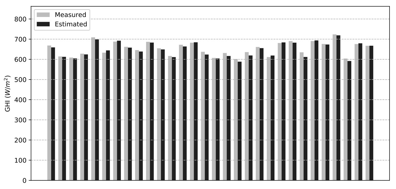 Figure 1
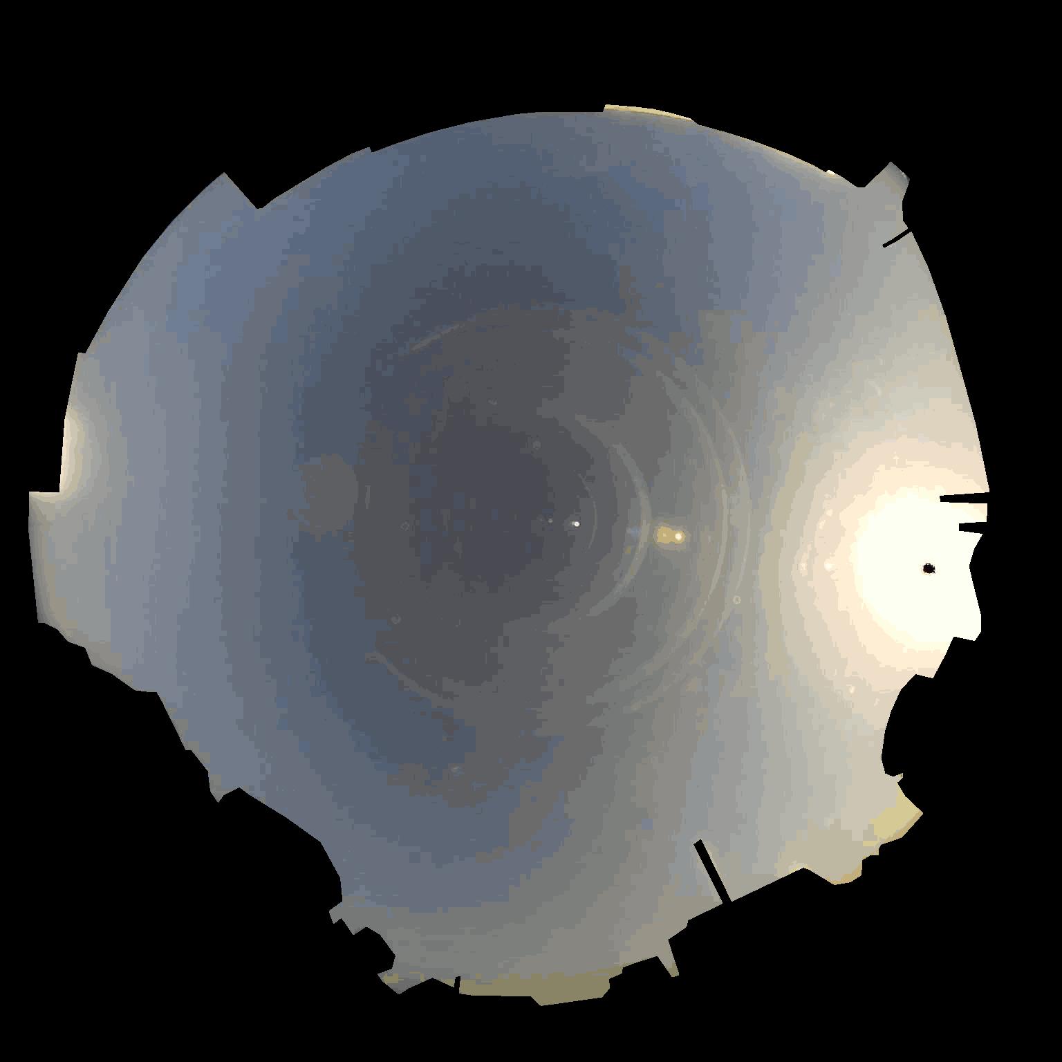 Figure 2
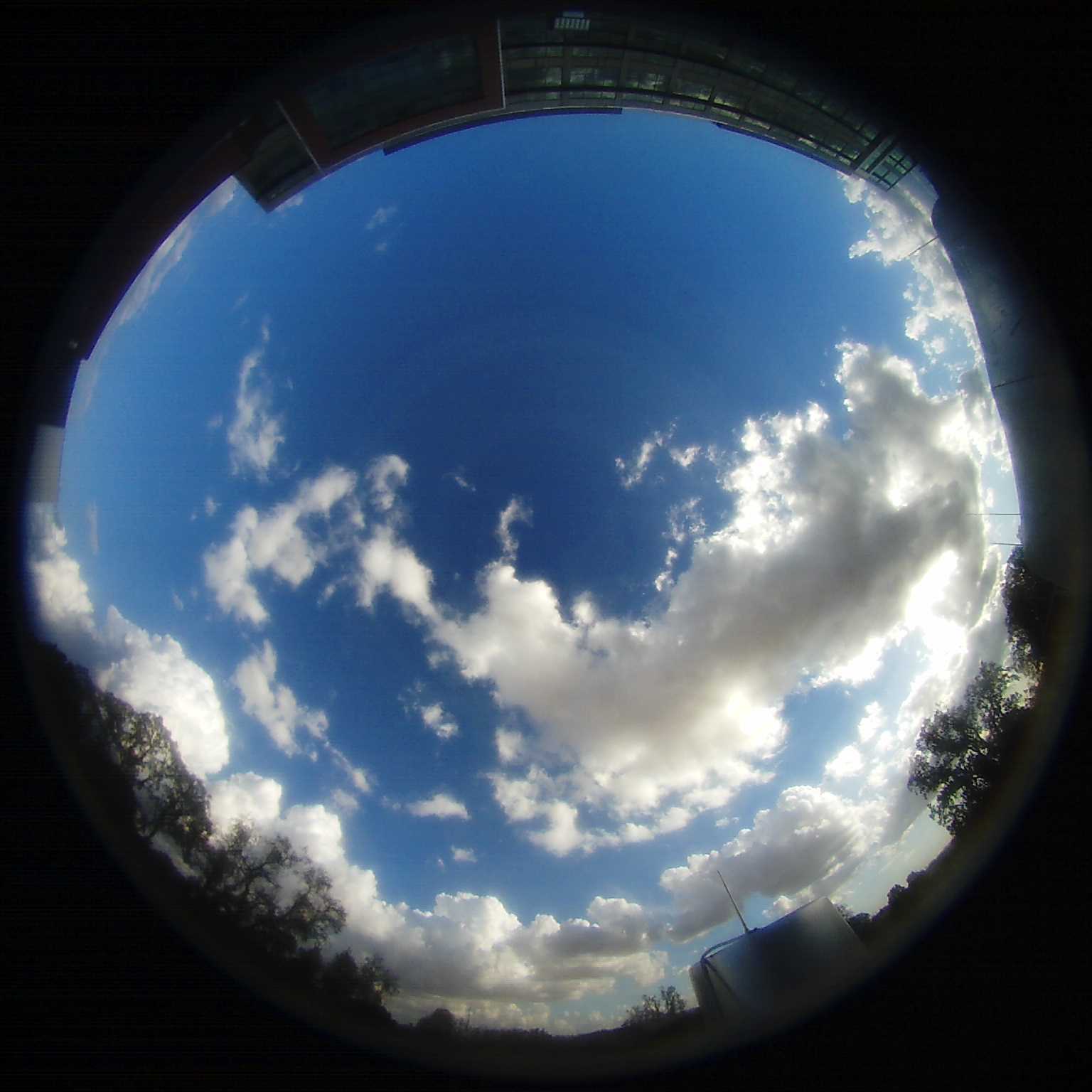 Figure 3
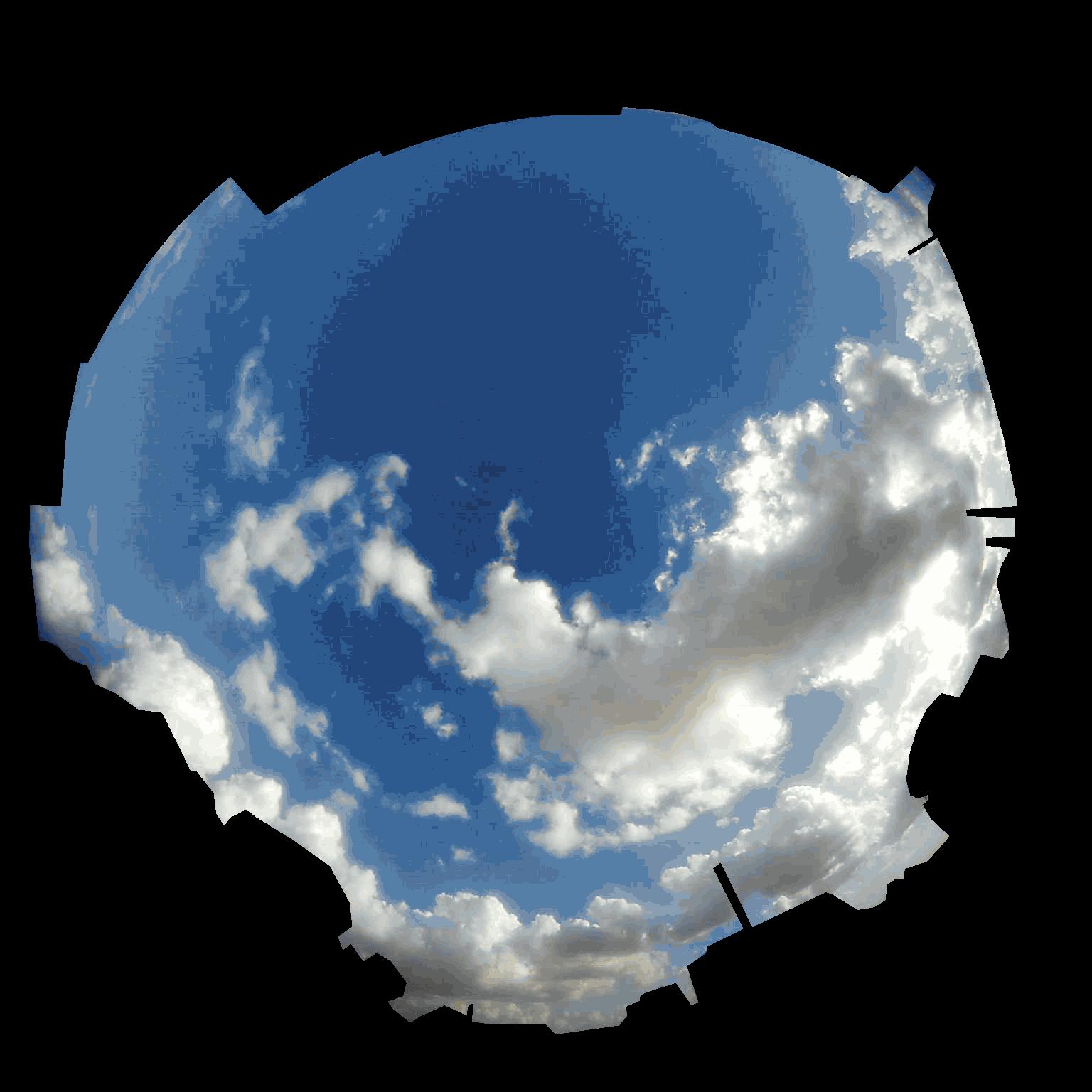 Figure 4
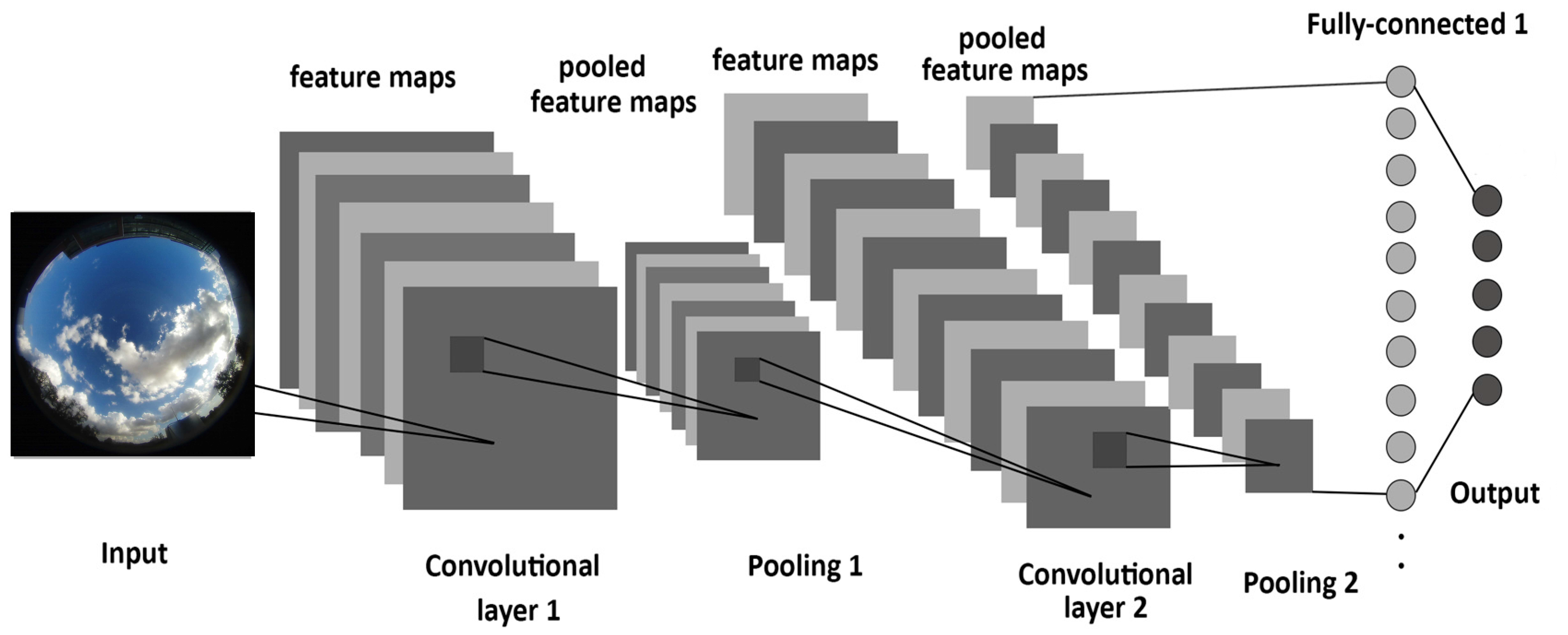 Figure 5
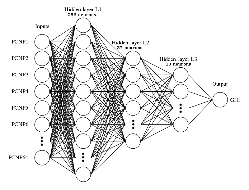 Figure 6
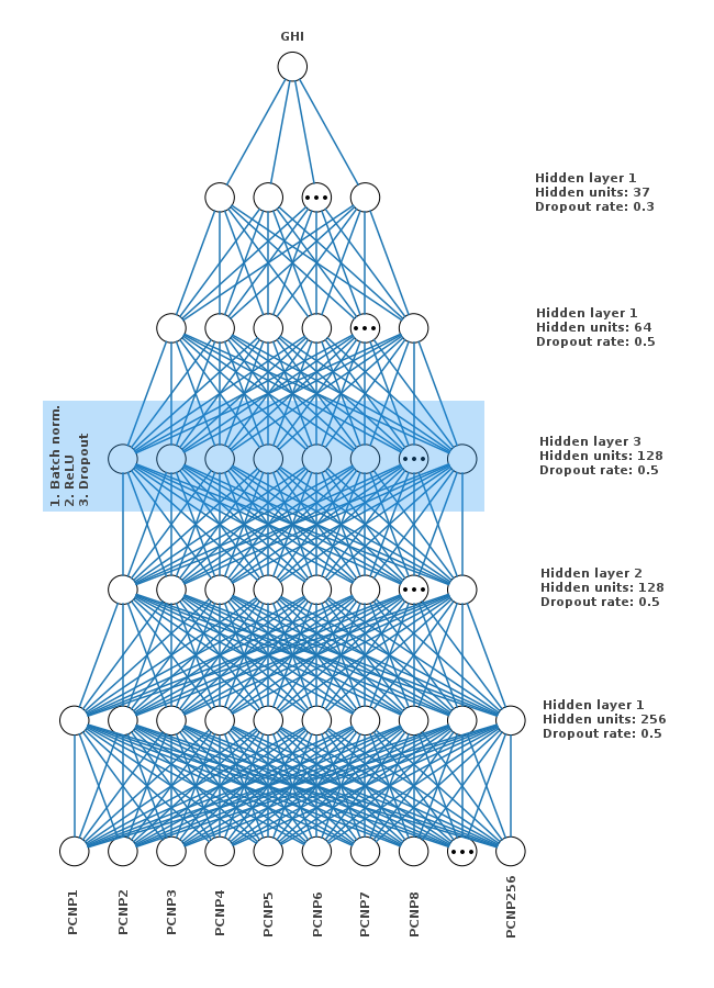 Figure 7
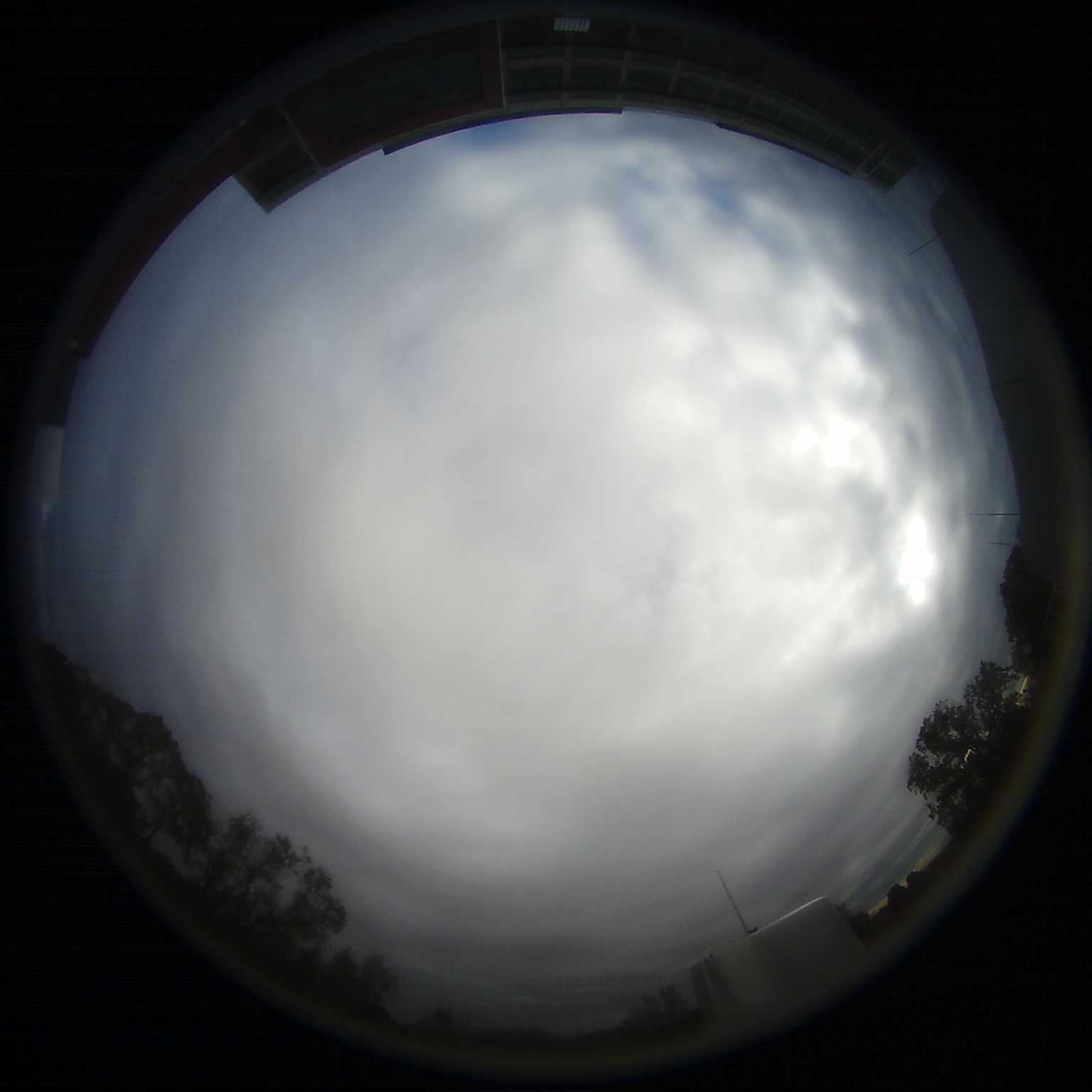 Figure 8
 Figure 9
 Figure 10
 Figure 11
| Parameter | Value |
|---|---|
| Features | |
| Target | sky class: “clear” or “cloudy” |
| Number of hidden layers | 1 |
| Number of hidden units | 27 |
| Activation function | sigmoid |
| regularization parameter | |
| Optimizer | Limited-memory BFGS |
| Parameter | Value |
|---|---|
| Features | |
| Target | GHI |
| Number of hidden layers | 5 |
| Number of hidden units | , , , and |
| Activation function | |
| Dropout rates | and for the last hidden layer |
| Optimizer | Stochastic gradient descent |
| Optimizer learning rate | |
| Optimizer momentum | Nesterov with parameter |
Peer Reviews
No public reviews on file for this paper yet. If you reviewed it on a platform where reviews are public (OpenReview, ICLR, NeurIPS, ICML), you can paste yours below so the community can read it here.
Videos
No videos yet. Explain this paper in a talk, walkthrough, or lecture? Add one.
Taxonomy
Methodsk-Means Clustering
Deep Learning for Inferring the Surface Solar Irradiance from Sky Imagery
Mehdi Zakroum1, Mounir Ghogho13, Mustapha Faqir1 and Mohamed Aymane Ahajjam1
1International University of Rabat, TICLab, Morocco
3University of Leeds, School of IEEE, UK
{mehdi.zakroum,mounir.ghogho,mustapha.faqir,aymane.ahajjam}@uir.ac.ma
Abstract
We present a novel approach to perform ground-based estimation and prediction of the surface solar irradiance with the view to predicting photovoltaic energy production. We propose the use of mini-batch -means clustering to extract features, referred to as per cluster number of pixels (PCNP), from sky images taken by a low-cost fish eye camera. These features are first used to classify the sky as clear or cloudy using a single hidden layer neural network; the classification accuracy achieves 99.7%. If the sky is classified as cloudy, we propose to use a deep neural network having as input features the PCNP to predict intra-hour variability of the solar irradiance. Toward this objective, in this paper, we focus on estimating the deep neural network model relating the PCNP features and the solar irradiance, which is an important step before performing the prediction task. The proposed deep learning-based estimation approach is shown to have an accuracy of 95%.
Index Terms:
photovoltaic, solar irradiance, sky imaging, machine learning, k-means clustering, deep learning, neural networks.
I Introduction
With the proliferation of photovoltaic (PV) energy systems, it is important to develop a reliable energy management system for operators to optimize the integration of PV energy into the electrical grid. Predicting the energy generated by the PV installation is a key feature in such a system, since it allows to detect faulty performance, to perform load scheduling, and in general to make better operational decisions [1]. Forecasting surface solar irradiance (SSI) is the basis of forecasting the PV energy because of the direct relation between these two.
If the sky is clear, physics-based prediction models perform well. Since some of the parameters in these models may be difficult to obtain, data-driven methods have been proposed to predict the SSI. For example, the Global Horizontal Irradiance (GHI) was shown to be accurately predicted with the nonlinear auto-regressive with exogenous inputs (NARX) model, having as input past GHI values [2].
Predicting the SSI in the case of a cloudy sky is much more challenging than in the case of clear sky conditions. This is due to the non-stationarity of the clouds introduced by the stochastic behaviour of the wind in the spatial (e.g. height of the clouds) and temporal dimensions. To address this issue, two categories of methods have been proposed in the literature: ground-based methods and geostationary satellite-based methods. Satellite-based prediction is primarily carried out using numerical weather prediction and satellite cloud monitoring. However, this approach only provides rough estimation due to the spatial and temporal resolution limitations of satellite images [3]. Ground-based methods, using sky imaging, have the potential to provide better performance, particularly for the prediction of intra-hour variability of the irradiance [4]. This is the approach adopted in this paper.
Toward the objective of forecasting the SSI, in this paper, we propose to use deep learning to accurately estimate the mapping function between the sky image and the corresponding irradiance, which is an important step before addressing the forecasting task. The data set used in this paper consists of sky images, taken with a low-cost fish eye camera, and their corresponding Global Horizontal Irradiance (GHI). First, the size of the images is reduced by clustering the colors of the images’ pixels into a relatively small number of color clusters; this is carried out using the mini-batch -means clustering algorithm. The resulting segmented sky image is used to classify the sky as either clear or cloudy; the classifier was learned using manually labeled images and a single hidden layer neural network. Using the cloudy sky image subset, a deep neural network is trained to model the relationship between the sky images and the corresponding irradiances.
II Data set
We use a data set consisting of RGB hemispheric sky images of size pixels, taken with a Vivotek FE8174 fish-eye camera, and their corresponding GHI, recorded with Kipp & Zonen CMP11 pyranometer. The data set was recorded during a period of three months (October, November and December of 2016) in Folsom, CA, USA. A record is taken every minute. More details about this data set can be found in [4]. Figure 1 shows a sample of three sky images corresponding to different weather conditions.
III Sky image segmentation and feature extraction
Segmenting an image consists of reducing it to salient pixels that reflect its global perceptual aspects. These representative pixels, also called super-pixels, define the segments of a reduced image. Each segment has a label, usually a color, and is present in one or more regions in the image. This task provides a convenient representation of the image for further analysis. It also serves to lower the computational cost because of the reduced number of values taken by the channels of the color model in use.
Our goal is to simplify the representation of the RGB sky images without losing much information about the three sky components, which are the clear sky, the clouds and the solar disk. These three sky components are represented by different sets of a relatively small number of RGB colors, with each one of them contributing to the GHI with a certain weight. For instance, clouds might have different levels of brightness, depending on the light they receive from the sun, going from white near the solar disk to dark gray in the surroundings. The intuition behind extracting different segments of the sky component is that we could infer the GHI by knowing the number of pixels of each segments of the segmented sky image. Indeed, a decrease in the GHI due the presence of clouds, particularly when (partially) obscuring the sun, is manifested in the segmented sky image by a reduction of the number of pixels present in the sun segments, an increase of the number of pixels in the cloud segments, and a reduction of the number of pixels representing the clear-sky.
Clustering is one of the commonly used methods to segment an image. The most widely used clustering algorithm is -means. The statement of the problem is as follows: given pixels in the -dimensional space defined by the R, G and B channels (the axes of the space), and an integer , find a set of super-pixels, so as to minimize the mean squared distance between each pixel and its nearest super-pixel. The caught super-pixels should be representative of all the colors present in the sky images of the whole data set, knowing that the colors vary with the time of day and the weather conditions, as depicted in Figure 1.
The standard version of the -means algorithm, first proposed by Lloyd [5], is suitable for relatively small data sets (which is not our case), because it requires to load all the images in memory before processing. A workaround to this memory limitation problem is to train the -means algorithm on a manually selected set of sky images that catch most of the typical colors representing the sky components. A better solution is to use the stochastic gradient descent implementation of the -means algorithm. To reduce the stochastic noise and thus allow convergence to better centroids, a mini-batch version of the stochastic gradient descent -means algorithms was proposed in [6]. Figure 2 shows clustered sky images using a trained -means model with . It is worth pointing out that before running the -means algorithm, a mask hiding the surrounding components which are not part of the sky is applied to the images in order to intercept exclusively sky pixels.
After training the mini-batch -means algorithm on the entire set of sky images, we perform the segmentation using the resultant centroids. Then, for each segmented image, we extract the number of pixels present in each segment. We refer to these features in the following sections as per cluster number of pixels (PCNP).
IV Sky image classification
Many studies in the literature used NARX neural networks to forecast the PV energy [1, 2]. Even though this model showed excellent ability in predicting the solar irradiance (and directly the PV energy) under clear sky conditions, there are no studies, to our knowledge, that cover the problem of the noise generated by the clouds that affects the solar irradiance, making the NARX model performance to degrade. The aim of this study is to enhance the prediction capabilities of such a model by taking into account the configuration of the sky. In order to decide about the prediction strategy, we first need a classifier that separates clear sky images from cloudy ones.
We use a data set consisting of sky images labeled manually, from which 75% serve as a training set and the remaining sky images as a testing set. The classifier is a single hidden layer neural network that takes as inputs the PCNP features extracted from the raw sky images and outputs two probability scores corresponfding to the two labels. We use the sigmoid function as neurons’ activations. The neural network is trained using Limited-memory BFGS algorithm which is known to converge to better solutions on small data sets. Table I outlines information about the classifier.
V GHI estimation
In this section, we estimate the transfer function between the extracted PCNP features and the measured GHI. The data set we use consists of 256 PCNP features (i.e. , with each feature representing the count of one of the super-pixels, and a target variable which is the GHI. The data set counts records after removing elements having a GHI of [math].
Our modeling approach utilizes a deep neural network. The model’s architecture consists of five hidden layers , …, having , , , and hidden units, respectively. We use as activation function the Rectified Linear Unit which gives better results than the hyperbolic tangent usually used in regression problems. Dropout regularization is applied to each hidden layer of the network during the training phase, which helps prevent over-fitting by reducing hidden units co-adaptation. This technique gives major improvement to our model over penalizing the weights with the regularization. We also apply batch normalization to each hidden layer in order to maintain the mean activation close to [math] and the activation standard deviation close to . This has the effect of accelerating the training phase by allowing the use of a higher learning rate. It should be pointed out that the PCNP features were preprocessed by scaling them to zero mean and unit standard deviation. Figure 3 depicts our deep neural network’s architecture.
The model is trained using Stochastic Gradient Descent algorithm with Nesterov momentum, which is better suited for our large data set. The hyper-parameters of the deep neural network such as the number of hidden layers and neurons, the activation function and the regularization parameters are determined using 10-fold cross validation. Table II summarizes the parameters of our model.
VI Results and discussion
The estimation of the transfer function between the PCNP features and the GHI shows on the testing set a coefficient of determination of . The corresponding mean absolute error on GHI estimation is about , where the measured GHI ranges from [math] to . These scores are validated using -fold cross validation.
Figure 4 shows the GHI output by the deep neural network versus the real values acquired by the pyranometer for different weather conditions. The entries are randomly selected from the testing set.
Concerning the neural network classifier, the metric we use to measure the model’s performance is the accuracy (i.e. the frequency with which predictions matches labels).
[TABLE]
The classifier shows an accuracy of % on the testing set and is able to distinguish between clear sky images having the glare surrounding the center (c.f. Figure 1a) and sky images having partial clouds. It is worth mentioning that the model may be improved by making it able to detect overcast sky conditions as well.
VII Conclusion and future work
In this paper, we presented a new method for modeling the relationship between hemispheric sky images and their corresponding surface solar irradiances. We first used mini-batch -means clustering in order to reduce the size of sky images. The extracted PCNP features were used an inputs to train a deep learning neural network to predict the irradiance associated with each sky image. A real dataset was used to illustrate the merits of the proposed method. As a future work, we will investigate how the extracted PCNP features can be used to forecast intra-hour variability of the irradiance in the case of cloudy and overcast sky conditions.
Acknowledgment
This research work was supported by the Institute for Research in Solar Energy and New Energies (IRESEN) and the United States Agency for International Development (USAID). The authors would like to thank Yinghao Chu, Hugo T. C. Pedro, Lukas Nonnenmacher, Rich H. Inman, Zhouyi Liao and Carlos F. M. Coimbra for providing the data set used in this paper.
The reference list from the paper itself. Each links out to its DOI / PubMed record.
- 1[1] M. Cococcioni, E. D’Andrea, and B. Lazzerini, “24-hour-ahead forecasting of energy production in solar PV systems,” in 2011 11th International Conference on Intelligent Systems Design and Applications , Nov 2011, pp. 1276–1281.
- 2[2] A. E. Hendouzi and A. Bourouhou, “Forecasting of PV power application to PV power penetration in a microgrid,” in 2016 International Conference on Electrical and Information Technologies (ICEIT) , May 2016, pp. 468–473.
- 3[3] C. W. Chow, B. Urquhart, M. Lave, A. Dominguez, J. Kleissl, J. Shields, and B. Washom, “Intra-hour forecasting with a total sky imager at the UC san diego solar energy testbed,” Solar Energy , vol. 85, no. 11, pp. 2881 – 2893, 2011.
- 4[4] Y. Chu, H. T. C. Pedro, L. Nonnenmacher, R. H. Inman, Z. Liao, and C. F. M. Coimbra, “A smart image-based cloud detection system for intrahour solar irradiance forecasts,” Journal of Atmospheric and Oceanic Technology , vol. 31, no. 9, pp. 1995–2007, 2014.
- 5[5] S. Lloyd, “Least squares quantization in PCM,” IEEE Transactions on Information Theory , vol. 28, no. 2, pp. 129–137, March 1982.
- 6[6] D. Sculley, “Web-scale k-means clustering,” in Proceedings of the 19th International Conference on World Wide Web , ser. WWW ’10. New York, NY, USA: ACM, 2010, pp. 1177–1178.