ALMA Observations of the massive molecular outflow G331.512-0.103 II: physical properties, kinematics, and geometry modeling
Carlos Herv\'ias-Caimapo, Manuel Merello, Leonardo Bronfman, Lars, \r{A}ke-Nyman, Guido Garay, Nadia Lo, Neal J. Evans II, Cristian, L\'opez-Calder\'on, Edgar Mendoza

TL;DR
This paper presents ALMA observations of the massive molecular outflow G331.512-0.103, analyzing its physical properties, kinematics, and geometry through detailed modeling, revealing an expanding cavity driven by stellar winds and a high-velocity outflow.
Contribution
It provides a comprehensive analysis of the outflow's physical conditions and models its geometry using 3D radiative transfer, advancing understanding of massive star formation processes.
Findings
Ambient medium density ~5x10^6 cm^-3 and temperature ~70 K.
Shock regions traced by SiO and SO2 have densities ~10^9 cm^-3 and temperatures 160-200 K.
Model successfully reproduces outflow and shell features using MOLLIE.
Abstract
We present observations and analysis of the massive molecular outflow G331.512-0.103, obtained with ALMA band 7, continuing the work from Merello et al. (2013). Several lines were identified in the observed bandwidth, consisting of two groups: lines with narrow profiles, tracing the emission from the core ambient medium; and lines with broad velocity wings, tracing the outflow and shocked gas emission. The physical and chemical conditions, such as density, temperature, and fractional abundances are calculated. The ambient medium, or core, has a mean density of cm and a temperature of K. The SiO and SO emission trace the very dense and hot part of the shocked outflow, with values of cm and K. The interpretation of the molecular emission suggests an expanding cavity geometry powered by stellar winds…
Click any figure to enlarge with its caption.
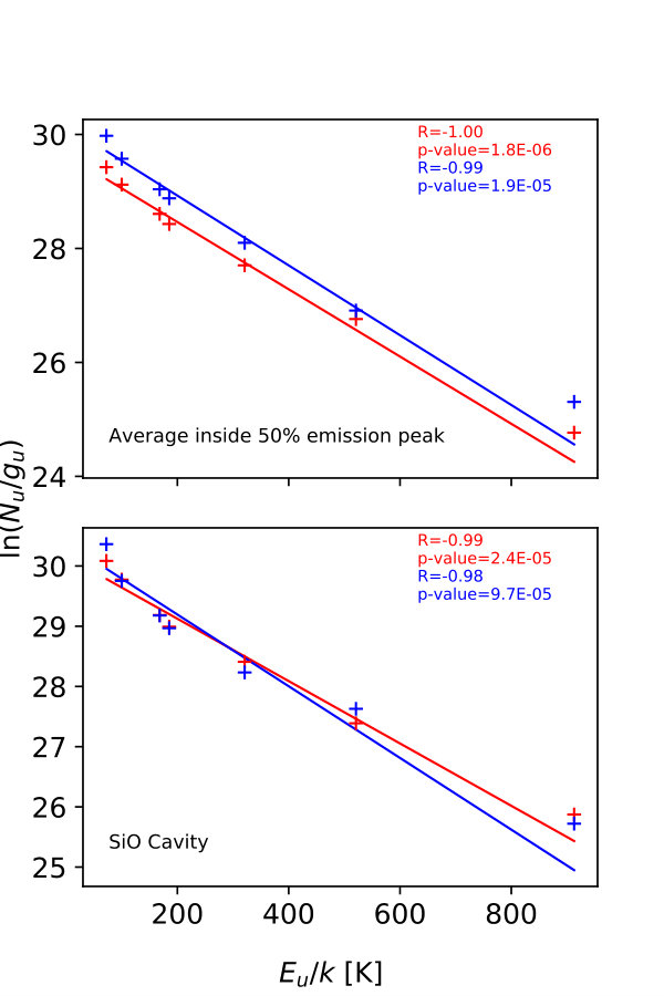 Figure 1
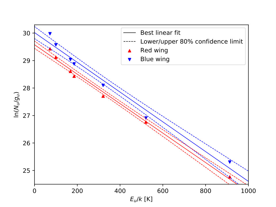 Figure 2
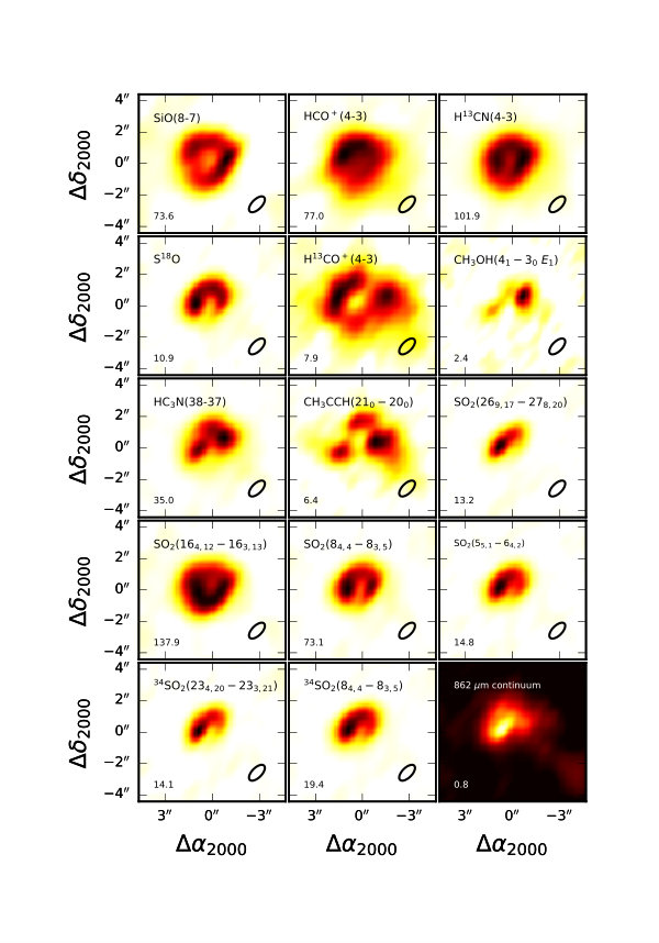 Figure 3
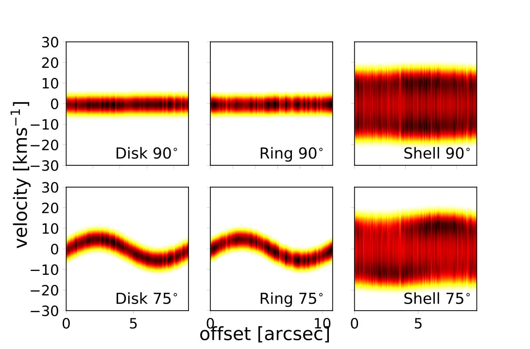 Figure 4
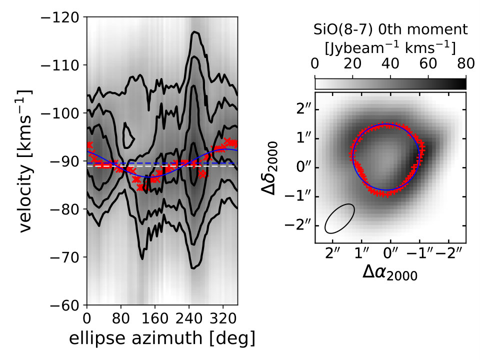 Figure 5
 Figure 6
 Figure 7
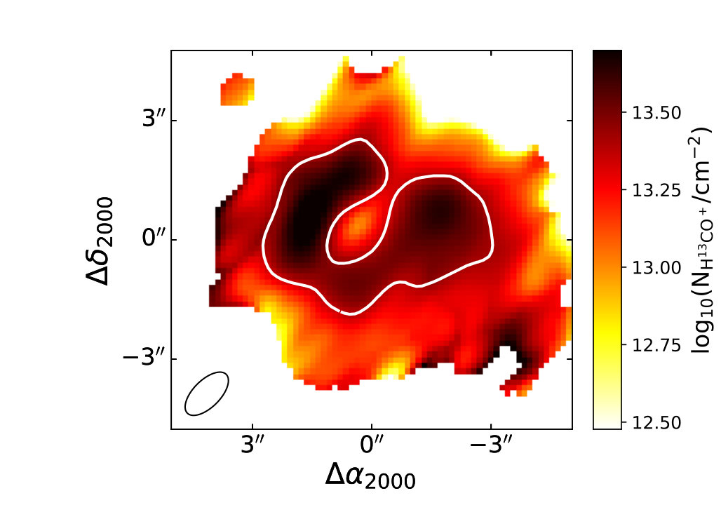 Figure 8
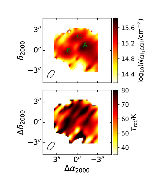 Figure 9
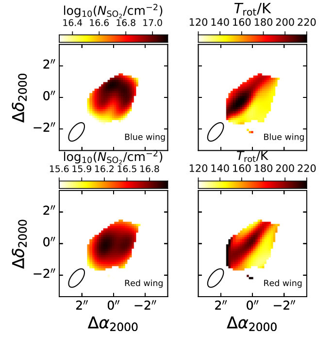 Figure 10
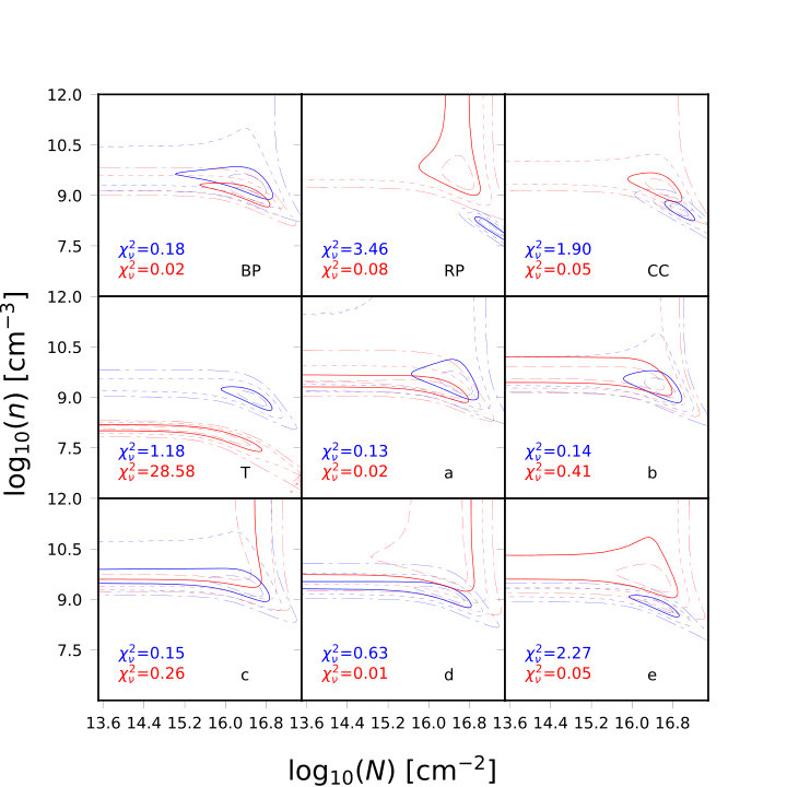 Figure 11
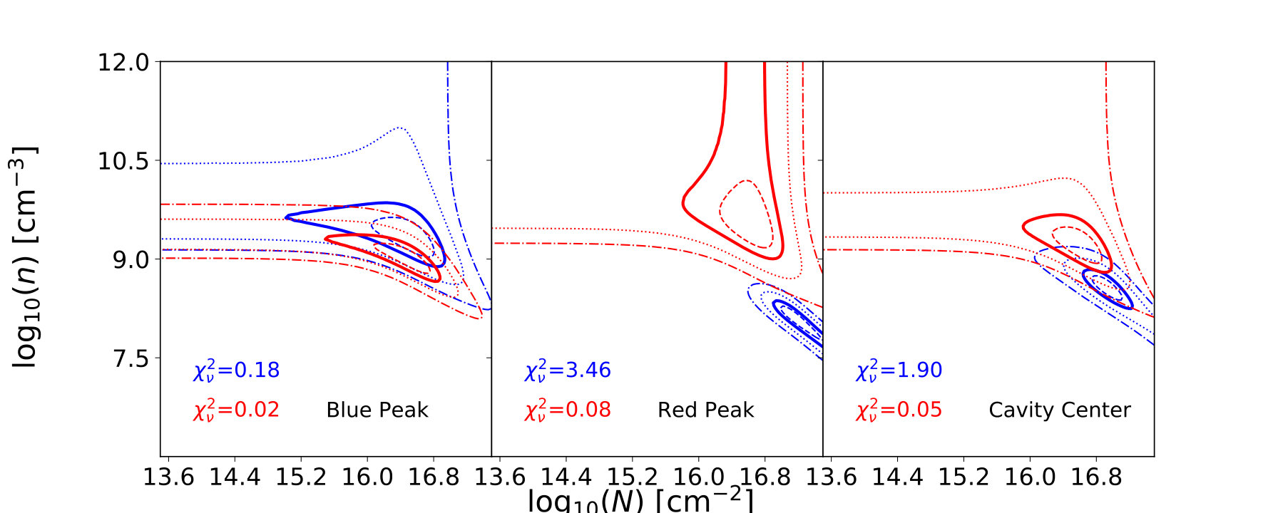 Figure 12
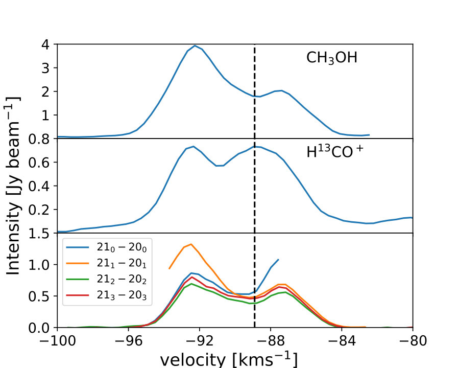 Figure 13
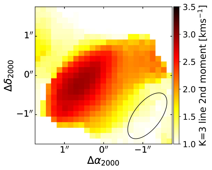 Figure 14
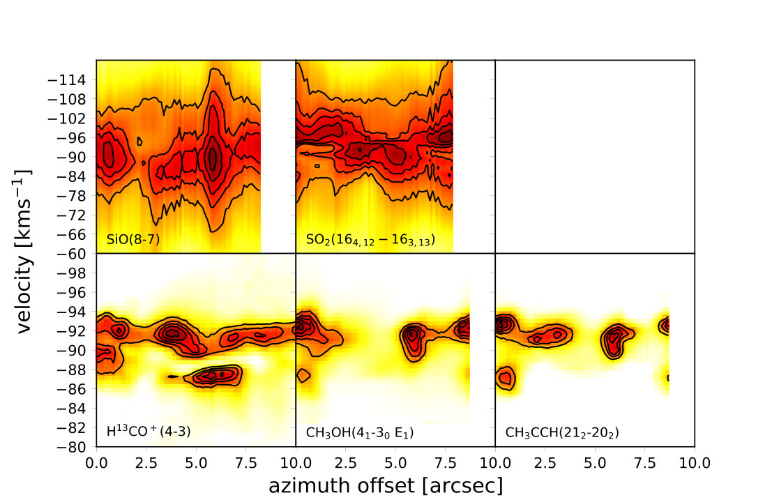 Figure 15
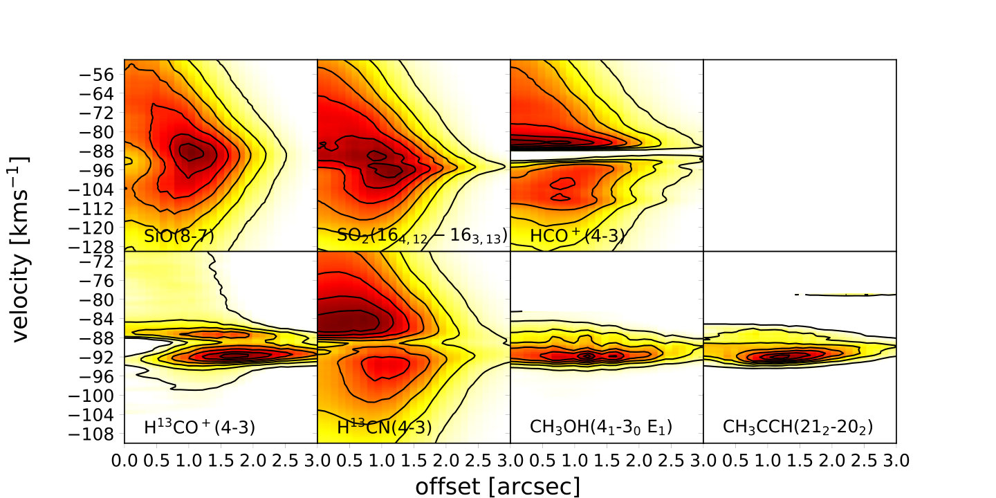 Figure 16
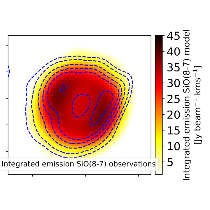 Figure 17
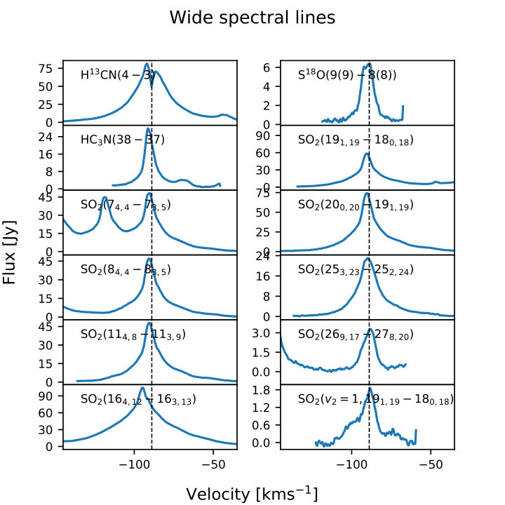 Figure 18
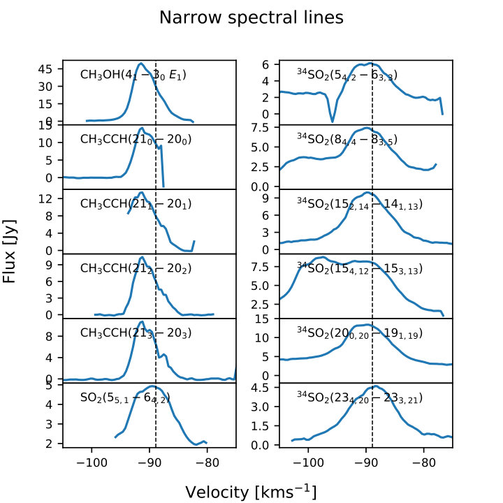 Figure 19
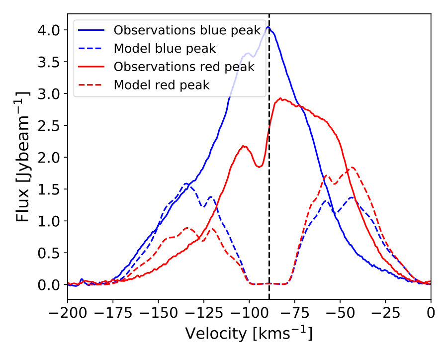 Figure 20
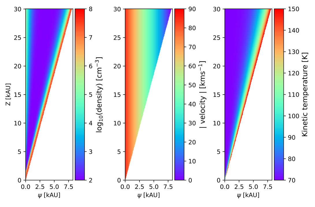 Figure 21
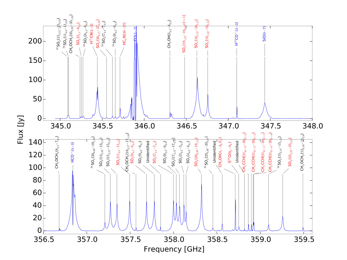 Figure 22
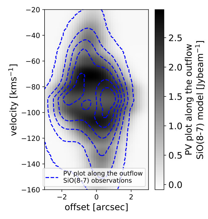 Figure 23
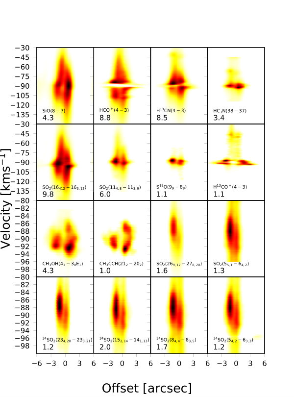 Figure 24
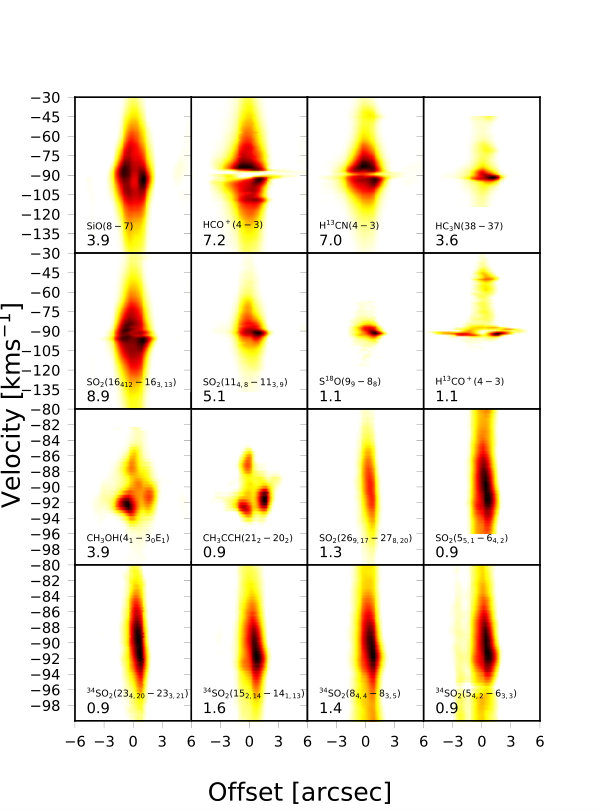 Figure 25
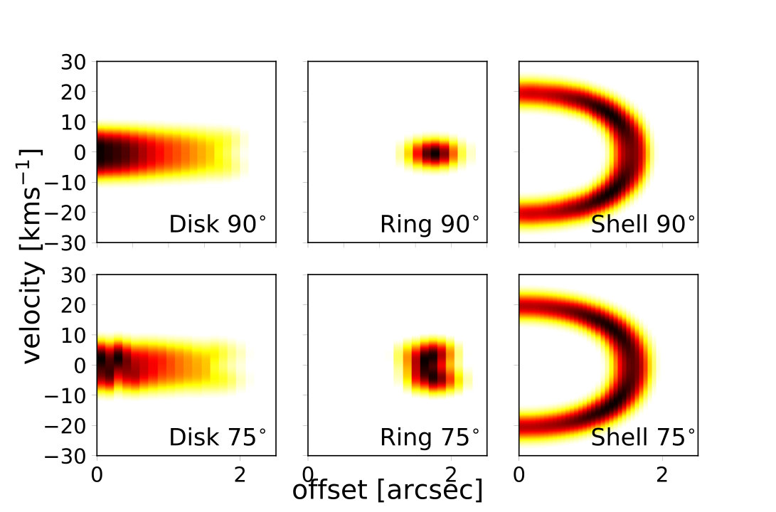 Figure 26
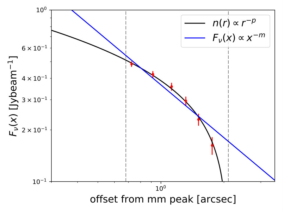 Figure 27
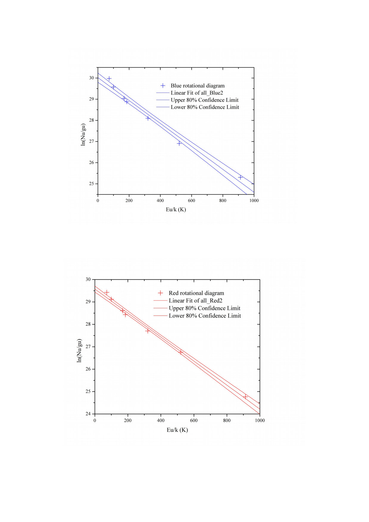 Figure 28
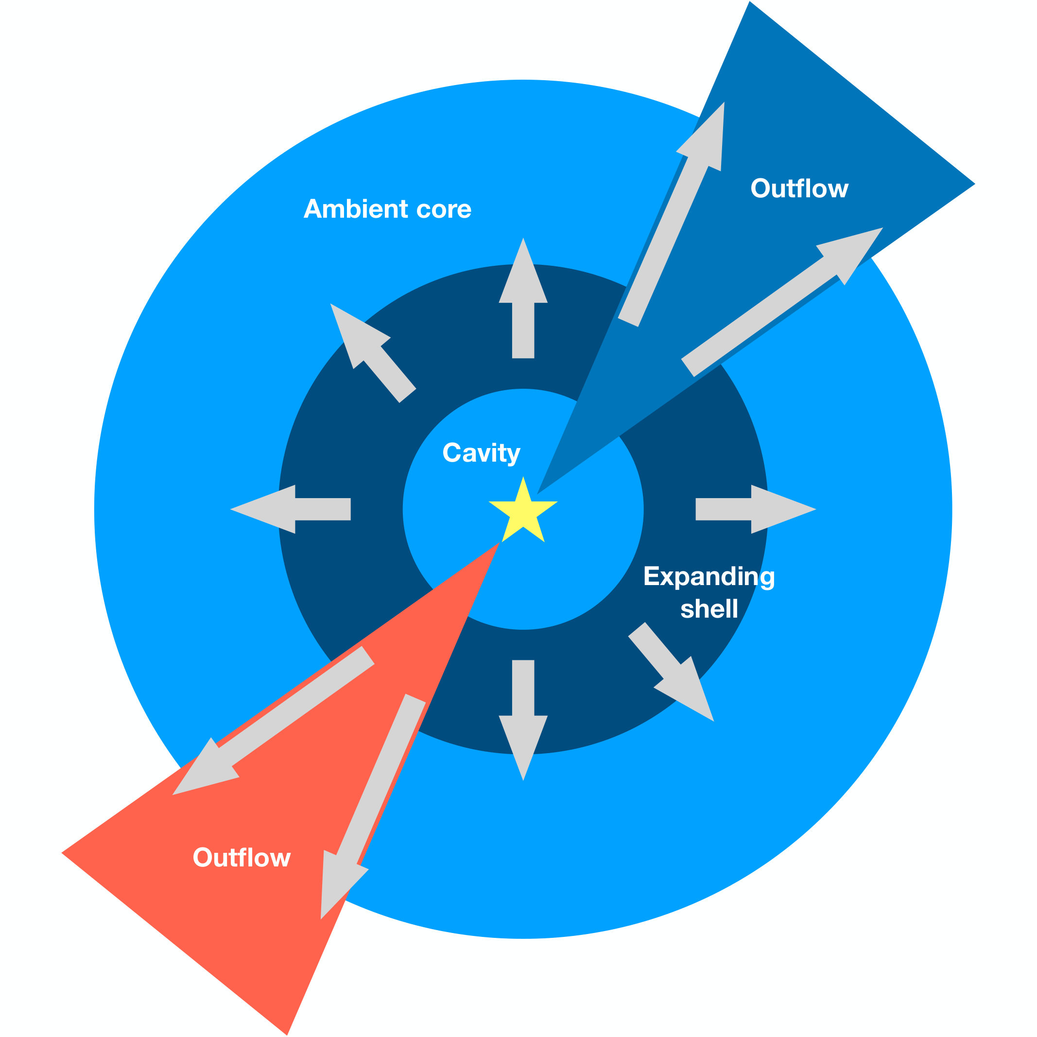 Figure 29
| Location | Using SiO | Using SO2 | ||
|---|---|---|---|---|
| Column density | Rot. temperature | Column density | Rot. temperature | |
| blue/red wing | blue/red wing | blue/red wing | blue/red wing | |
| [ cm-2] | [K] | [ cm-2] | [K] | |
| 50% emission peak | / | / | / | / |
| cavity | / | / | / | |
| blue peak | / | / | / | |
| red peak | / | / | / | |
| G331, =70 K | G331, =400 K | G5.89-0.39 | Orion-KL | G34.26+0.15 | |
|---|---|---|---|---|---|
| SiO | |||||
| SO2 |
| Location | ||||
|---|---|---|---|---|
| J2000 | J2000 | [cm-3] | [cm-2] | |
| SiO blue peak | 16:12:09.91 | -51:28:37.4 | ||
| SiO red peak | 16:12:10.08 | -51:28:37.6 | ||
| SiO cavity center | 16:12:09.99 | -51:28:37.5 |
| Parameter | Value |
|---|---|
| Center J2000 | 16:12:10.0 -51:28:37.4 |
| Line of sight angle | -8∘ |
| Position angle | 72∘ |
| Radius | |
| Expansion velocity | 21 km s-1 |
| Systemic velocity | -90 km s-1 |
| Property | Value |
|---|---|
| Distance | 7.5 kpc |
| Mass of core | |
| Mass outflow lobes | each |
| Kinetic age | yrs |
| Velocity range of the outflow | kms-1 |
| Expansion velocity of cavity | kms-1 |
| Mean density | cm-3 |
| Density power law index | |
| Temperature of core | K |
| Outflow inclination |
Peer Reviews
No public reviews on file for this paper yet. If you reviewed it on a platform where reviews are public (OpenReview, ICLR, NeurIPS, ICML), you can paste yours below so the community can read it here.
Videos
No videos yet. Explain this paper in a talk, walkthrough, or lecture? Add one.
ALMA Observations of the massive molecular outflow G331.512-0.103 II: physical properties, kinematics, and geometry modeling
Carlos Hervías-Caimapo1,2⋆, Manuel Merello3, Leonardo Bronfman1, Lars Åke-Nyman4, Guido Garay1, Nadia Lo1, Neal J. Evans II5,6, Cristian López-Calderón4, and Edgar Mendoza3
1Departamento de Astronomía, Universidad de Chile, Casilla 36-D, Santiago, Chile
2Jodrell Bank Centre for Astrophysics, School of Physics and Astronomy, University of Manchester, Oxford Road, Manchester M13 9PL, UK
3Universidade de São Paulo, IAG Rua do Matão, 1226, Cidade Universitária, 05508-090, São Paulo, Brazil
4Joint ALMA Observatory (JAO), Alonso de Córdova 3107, Vitacura, Santiago, Chile
5Department of Astronomy, The University of Texas at Austin, 2515 Speedway, Stop C1400, Austin, TX 78712-1205, USA
6Korea Astronomy and Space Science Institute, 776 Daedeokdae-ro, Yuseong-gu, Daejeon, 34055, Republic of Korea
Abstract
We present observations and analysis of the massive molecular outflow G331.512-0.103, obtained with ALMA band 7, continuing the work from Merello et al. (2013a). Several lines were identified in the observed bandwidth, consisting of two groups: lines with narrow profiles, tracing the emission from the core ambient medium; and lines with broad velocity wings, tracing the outflow and shocked gas emission. The physical and chemical conditions, such as density, temperature, and fractional abundances are calculated. The ambient medium, or core, has a mean density of cm*-3* and a temperature of K. The SiO and SO2 emission trace the very dense and hot part of the shocked outflow, with values of cm*-3* and K. The interpretation of the molecular emission suggests an expanding cavity geometry powered by stellar winds from a new-born UCHII region, alongside a massive and high-velocity molecular outflow. This scenario, along with the estimated physical conditions, is modeled using the 3D geometry radiative transfer code MOLLIE for the SiO(J) molecular line. The main features of the outflow and the expanding shell are reproduced by the model.
Subject headings:
ISM: clouds — ISM: molecules — ISM: jets and outflows — stars: formation
1. Introduction
The formation of massive stars is an important topic in stellar astrophysics that is open for debate. Despite the wealth of knowledge that has been obtained on young massive stellar sources, still there is no universal agreement on how massive stars are formed and evolve (Garay & Lizano, 1999; Zinnecker & Yorke, 2007; Kennicutt & Evans, 2012).
There is an accepted paradigm on how low-mass stars form and evolve (Shu et al., 1987). However, problems such as scarcity of young sources, large heliocentric distances (several kpc in some cases) and the lack of appropriate spatial resolution (that has been addressed with interferometers such as ALMA just in recent years) make the subject of formation of massive stars an open question. Two main theories compete on trying to explain this mechanism: the monolithic gravitational collapse/turbulent core accretion model (McKee & Tan, 2003), which is basically the extension of the model of formation of low-mass stars to the massive ones, but with higher accretion rates and energetics; and the competitive accretion model (Bonnell et al., 2001, 2004), which states that low-mass seeds that will eventually form massive stars compete for the available gas in the gravitational potential of their native cluster.
Since massive stars have very short lifetimes, sources that are currently in the process of formation are very valuable. Molecular outflows are commonly detected toward protostellar objects, and observed physical properties such as outflow power, force and mass loss rate, seems to correlate over a large range of luminosities, suggesting that outflows found in massive star forming regions are a scaled-up version of those found in their low-mass star counterparts (Tan et al., 2014). The injection of momentum and energy from outflows are important in star forming regions at small and large spatial scales, although the role of feedback at different stages of protostellar evolution is still not clear (Frank et al., 2014; Bally, 2016). Thus, from an observational point of view, a principal objective is to identify and characterize examples of young, massive and powerful outflow-associated sources, as is the case for the work here.
The present work focuses on arcsecond-resolution ALMA observations of the massive molecular outflow G331.512-0.103 (Bronfman et al., 2008). This source is located in the tangent of the Norma spiral arm, at a heliocentric distance of kpc, and corresponds to a bright MYSO object associated with the central region of the G331.5-0.1 giant molecular cloud (García et al., 2014, with a H2 mass of M*⊙*), which shows evidence of ongoing massive star formation (Merello et al., 2013b, which we will refer to as MM13b). There are several characteristics that make this object valuable and unique: the presence of very broad emission wings in CO, CS and SiO, which indicate the presence of a very powerful outflow; the compact emission (not resolved at resolution with APEX, Bronfman et al., 2008), which we interpret as the outflow lobes being closely aligned with the line of sight; an expanding bubble geometry, which indicates the presence of stellar winds possibly arising from the exciting star within the hyper compact HII region (Merello et al., 2013a, which we will refer to as MM13a); and high energetics, which makes this source one of the most powerful massive outflows discovered. For example, in the compilation of outflows in O-type young stellar objects by López-Sepulcre et al. (2009), only five objects have higher bolometric luminosity.
Part of the ALMA observations and the main results are summarized in MM13a. The SiO(J) and CO(J) lines show broad velocity wings ( kms*-1*). The SiO line shows ring-like emission, suggesting an expanding motion, probably a cavity being blown-out by the powerful stellar output from the central source. The H13CO+(J) line traces the systemic velocity structure, as well as the surrounding core with its narrow emission.
This work is the follow-up of MM13a. Here we investigate for the first time 18 newly analyzed lines, along with the 4 already analyzed there, with the goal of characterizing the physical conditions, kinematics and morphology of the massive molecular outflow. In this new work, we analyze the SiO and SO2 molecules, widely recognized as outflow tracers (Schilke et al., 1997b); CH3CCH, which thermalizes at densities of cm*-3* and is a very good estimator of temperature (Fontani et al., 2002; Molinari et al., 2016); and SO isotopologues, which are tracing the hot-core chemistry (Charnley, 1997; Wakelam et al., 2004). The paper is organized as follows: Section 2 describes the ALMA band 7 observations, giving the main parameters of the observed spectral lines. Section 3 presents the results of the observations, including integrated emission maps and position-velocity plots. Section 4 presents the analysis of physical conditions, geometry, and kinematics performed on the source. A 3D radiative transfer model of the SiO(J) line is also included. Our conclusions are summarized in Section 5.
2. Observations
The observations were performed with the Atacama Large Millimeter/submillimeter Array (ALMA) during Cycle 0, as described in MM13a. The primary beam was and the synthesized beam was , with a position angle of . The interferometric observations miss the recovery of large spatial scales above .
The data were processed using the Common Astronomy Software Application (CASA; McMullin et al., 2007). The four spectral windows (SW) are centered at 345.8, 347.2, 357.3 and 358.6 GHz, each extending over 1875 MHz and consisting on 3840 channels. The generated maps considered a “briggs” weighting mode on the data (robust parameter = 0.5).
Figure 15, in Appendix A, shows the composite spectra of SW3-SW2 (top), and SW0-SW1 (bottom), integrated over a region of centered at , . The identified lines are marked across both bands. The image shows several blended lines that required a careful channel-by-channel determination of the emission mask during the cleaning reduction process. The rich spectra exhibit sulphur-bearing, carbon chains and other complex molecules, characteristic of hot core line emission found toward other well-studied sources at similar frequency bands, such as Cepheus A East (e.g., Brogan et al., 2007, 2008), Orion KL (Schilke et al., 1997a), and G5.89-0.39 (e.g., Hunter et al., 2008).
For the present work, we focus on 18 (new) + 4(from MM13a) lines, including, among others, the hot-core chemistry/shock tracer SO2, a K-ladder of four CH3CCH lines (commonly used as a source temperature test), the optically-thin line H13CN probing densities up to cm*-3*, and HC3N, which is found toward warm and dense regions such as hot cores, where it is shielded against destruction by photo-dissociation and C+ ions (Rodriguez-Franco et al., 1998; Prasad & Huntress, 1980). Figure 1 shows the integrated spectrum of each of these lines as a function of velocity (the systemic velocity of the source is kms*-1*). A couple of these lines appear blended or contaminated with emission at similar frequencies. We leave the analysis of the rest of the lines observed in the spectra, mostly associated with complex organic molecules such as dimethyl ether (CH3OCH3) and ethyl cyanide (C2H5CN), for upcoming studies.
The H13CO+() line shows a secondary peak of emission at kms*-1*. MM13a reports this as a “molecular bullet”, or gas expelled at very high velocity by the powerful energetics of the outflow. Their presence has been reported previously in star formation region outflows (Tafalla & Bachiller, 2011). However, once we analyzed the full band and the other lines contained in it, this might be no longer the case. A line with an excited vibrational level, HC3N(,) at 346.9491233 GHz, matches with this secondary peak. Other star forming regions, observed at similar frequencies, show the presence of this line (Brogan et al., 2008; Nagy et al., 2015). We also observed, in our band-7 data, the HC3N() line at 345.60901 GHz. Comparison between them in velocity and morphology might indicate that both belong to emission of the same molecule, so the presence of a molecular bullet can be discarded, instead appearing to be another line that was not recognized in the first analysis of the ALMA data.
3. Results
3.1. Moment 0 maps
Figure 2 shows imaging of the 0th moment maps of emission, integrated in the velocity range to km s*-1* (systemic velocity range).
In the integrated spectra, from Figure 1, we can identify two groups of lines. The first group (labeled wide lines) are the ones with broad velocity wings. They are the SiO, S18O, HCO+, H13CN, HC3N, and most of the SO2 lines. At the systemic velocity, most of these lines, especially the SiO emission, trace an emission with a ring-like shape (see Figure 2).
The second group (labeled narrow lines) includes lines that have narrow emission at systemic velocity. They are the CH3CCH, CH3OH, and H13CO+ lines 111H13CO+ also shows evidence of high-velocity wings, but with a signal-to-noise ratio .
Spatially, the emission from all lines comes roughly from the same central region, shown in Figure 2, with a diameter of . Most of the lines trace the ring-like emission that is clearly seen at the systemic velocity.
The 862 m continuum emission is shown in Figure 2 as the inverted color map in the bottom right corner. It is composed of a single peak that almost coincides with the center of the SiO emission ring, and weaker emission that follows the edge of the ring feature.
{turnpage}
3.2. Position-velocity (PV) plots
To study the gas kinematics traced by the line emission, we made PV plots of most of the observed lines along two axes: parallel and perpendicular to the outflow axis with a position angle of , as defined in MM13a. A “slit” of 11 pixels () is used. Both kinds of PV plots are shown in Figure 3.
4. Analysis
We interpret the wide group of lines as tracers of shocked high-velocity hot gas. The narrow group of lines trace the ambient core cold gas emission at the systemic velocity. As reported in MM13a, we interpret the kinematics seen in the PV plots of SiO as an expanding shell.
We present our interpretation of the source, shown in Figure 4. The bipolar outflow is outlined by emission from shock tracers, such as SiO and SO2. We consider the presence of an expanding shell, which we interpret as shocked gas material being blown out by the stellar wind from the ultra compact HII region at the center. The ring-like emission we see in the maps of the lines would correspond to this expanding shell. The narrow group of lines traces emission at systemic velocities (e.g. CH3CCH) and the ambient dense and warm gas core.
4.1. Physical conditions
4.1.1 Estimation of column density and temperature
*SiO analysis - * Assuming a common for the SiO transitions and that they are optically thin, we calculate the column densities of the outflow wings. See, for example, the analysis in the similar outflow source W51 North (Zapata et al., 2009). In this ALMA data set, we only have observed one line of SiO at high resolution. Therefore, for the excitation temperature value, we consider the estimate from MM13b, using only two transitions of SiO, obtained with APEX, for each outflow wing: K (blue wing) and K (red wing).
The estimated averaged column densities are listed in Table 1. The significant values are the ones calculated in the blue and red peak, cm*-2* and cm*-2*, respectively, which are taken as the column densities of the outflow wings. Estimating the size of the emission from the 50% peak contour level in the 0th moment maps in the blue and red peaks, and using an abundance of (see Section 4.1.2), we estimated the masses to be , for each outflow wing. This value is about half of the mass calculated for the wings in Bronfman et al. (2008), with CO.
*SO2 analysis - * One of the principal molecules observed in the ALMA data set corresponds to SO2, since several transitions fall in the observed bandwidth. In this case, assuming optically thin emission, we use the rotational diagram technique (Linke et al., 1979; Goldsmith & Langer, 1999) to obtain its column density and rotational temperature.
The partition function for SO2 is (Claude et al., 2000)
[TABLE]
where =60778.5511 MHz, =10317.96567 MHz and =8799.80750 MHz.
Since some SO2 lines are blended, a compromise must be reached between the range of the wings to be used and the number of lines. In the ideal case, one wants to include the complete width of the wings and use as many lines as available. Using a narrow range of velocities is not advisable since the column density is underestimated. Two SO2 lines (J= and J) were discarded since they are blended. Another line (J) has a clear excess over the other lines, and may be contaminated by an unknown line. In total, 7 lines were used in the blue and red wings.
We consider the spatially averaged spectrum inside the contour of the 50% of the peak emission, as well as inside a circle with of diameter (corresponding to one beam) centered in the blue wing peak, the red wing peak, and the cavity center. These circles average roughly 40 pixels from the original data cube. With the averaged spectra in these four locations, we calculate the rotational diagrams and fit a straight line with a linear regression, from which we estimate column densities and rotational temperatures, listed in Table 1. The 1 errors are calculated from the covariance matrix from the linear fit. The blue and red peaks show the highest column density, of and cm*-2*, respectively. This is consistent with the same tendency observed in SiO. The average rotational temperature in the SO2 emitting region is K. The red peak is hotter than the blue peak, 202 and 146 K, respectively. As an example, in Figure 5, we show the SO2 rotational diagram for the flux averaged inside the 50% peak emission contour. For the linear fit, we consider a conservative error of 20% for the values. We show the 80% confidence intervals.
The estimated SO2 column density and rotational temperature maps for each outflow wing are shown in Figure 6. The ring-like emission is traced in SO2 by the blue and red wing emission. The rotational temperature maps show an elongated peak at K on both wings. The bright peak of emission, seen in most of the SO2 lines, corresponds to the peak in temperature in the blue wing, and also seen in in the red wing. This means that SO2 is likely tracing the most dense, hot, and shocked part of the proto-stellar core.
4.1.2 Fractional abundances
One physical parameter that is hard to measure, yet needed for modeling is the fractional abundance of each molecule. The fractional abundance , where stands as a particular molecule, is measured as where is the column density of the correspondent molecule.
In order to calculate the fractional abundances, some evaluation of the mass is needed. The virial mass can be used to estimate it (e.g. Shirley et al., 2003), or the mass estimated from the thermal continuum emission, the dust mass, can also be used (e.g. Fontani et al., 2002). The latter method is used in this work, and the mass is calculated from the 862 m continuum emission.
The equation to calculate the gas mass from dust thermal continuum, when the emission is optically thin, is
[TABLE]
where is the observed flux, is the dust mass coefficient, is the distance to the source, is the Planck function, is the dust temperature and is the gas to dust ratio, which is uncertain, but usually set to 100 in the literature. The following values will be used: cm2g*-1* (interpolated from model OH5 in Ossenkopf & Henning, 1994) and kpc. On the other hand, the gas mass () can be estimated from
[TABLE]
where is the mass of the hydrogen atom times the mean molecular weight (that accounts for a fraction of helium, equal to 2.29), is the area of the emitting region (which must be consistent with the area used to calculate the dust flux ) and corresponds to the measured column density of the molecule . Equating to , and using the fact that corresponds to the solid angle that the source subtends, we have
[TABLE]
One quantity that is highly uncertain and sensitive for the dust mass estimation is the dust temperature. MM13b estimates the dust temperature to be 35 K, based on the Spectral Energy Distribution (SED) of the source. This value is for the entire clump though, so the dust temperature at the ALMA resolution is probably higher. A rotational diagram analysis of the CH3CCH lines shows that the ambient core temperature is K. MM13a uses an equilibrium dust temperature of 400 K within the central arcsec. We use these two limits to calculate a range of possible abundances, listed in Table 2.
We compare our fractional abundances results with similar sources studied in the literature. As stated in MM13a, one of the most similar sources to G331.512-0.103 is G5.89-0.39, an UCHII region which exhibits a powerful and compact bipolar molecular outflow. Klaassen et al. (2006) mapped this outflow with the James Clerk Maxwell Telescope (JCMT) at . The fractional abundances for SiO and SO2 are listed in Table 2, column 4. The Orion-KL region (Genzel & Stutzki, 1989) has shown chemical richness. Tercero et al. (2010) and references therein, reported a spectral line survey in the 90-300 GHz range. We list their fractional abundances, for comparison, in Table 2, column 5. Similarly, the UCHII region G34.26+0.15 (Garay et al., 1986; Wood & Churchwell, 1989) is also a well studied massive star forming source. For comparison, the fractional abundances are listed in Table 2, column 6.
4.1.3 Density and column density estimation with RADEX
The radiative transfer code RADEX (van der Tak et al., 2007) is a non-LTE radiative code that uses radiative/collision rates information and basic geometries to solve the statistical equilibrium and radiative transfer equations, estimating the intensities of several transitions of the most typical molecules observed in the sub-mm range.
Since the statistical equilibrium/population levels and the radiative transfer/radiation field are coupled, RADEX uses the Large Velocity Approximation (LVG) approximation by Sobolev (1960), where the mean intensity is expressed as a function of the source function and a photon escape probability . All the knowledge of the geometry/optical depth goes into this probability . An estimate is given by
[TABLE]
which coincides with the expression for a radially expanding sphere.
The procedure consists of using the integrated intensity ratio of several SO2 lines to constrain the physical parameters (e.g. Fu et al., 2012). Since RADEX does not include data on every SO2 transition, and also some lines of SO2 cannot be used (they are blended with neighboring lines in the blue and/or red wing), only 4 lines were used for this analysis. The lines should be as far away as possible in terms of energy, for the same reason that in the rotational diagram case. Two of them have low and two of them have high upper-level energies (), hence 4 line ratios are defined: (J)/(J), (J)/(J), (J)/(J) and (J)/(J).
The code needs several input values. Density and column density are left as free parameters. The kinetic temperature is fixed to K, which is the value constrained by SO2. The line-width is set to km s*-1*, which is the average of the FWHM of the 4 lines. The background temperature is set to K. The main collision partner that RADEX handles is H2. The output of the code for each pair of density and column density values are the line temperature , the excitation temperature , the optical depth of the line and the integrated intensity assuming a Gaussian shape. The latter is used to calculate the line intensity ratio.
Our method is similar to the one used by Plume et al. (1997) and van der Tak et al. (2000). It consists of the following: given line ratios (in this case ) and given the RADEX model that will predict line ratios as a function of density and column density, the quantity that must be minimized is
[TABLE]
where stands for each of the defined 4 ratios, is the observed line ratio, is the RADEX modeled line ratio and is an estimation of the error in the line ratio.
The wing emission in the SO2 lines must be used to measure the line ratios. These ranges were set as to km s*-1* for the blue wing and to km s*-1* for the red wing. These limits are slightly different than the ones defined in Section 4.1.1, since we are considering a subset of SO2 lines. We estimate the errors in the following way: the error due to the RMS of the spectra is %. The calibration error (phase and bandpass) is %. Considering an error of 15% in the integrated intensity, the resulting error in line ratios is %, which will be the adopted value. For each location, the averaged spectra within a circle of of diameter was used, which corresponds to roughly the size of one synthesized beam. Three relevant locations were chosen: the center of the cavity, as well as the red and blue peaks defined by the SiO emission. Their coordinates are listed in Table 3.
Using the standard interpretation of the space, the confidence levels are estimated as contours at chosen . The results for each of the locations probed are shown in Figure 7. The contours corresponding to 0.5, 1, 2, and 3 are shown as dashed, solid, dotted, and dashed-dotted lines, respectively. The results are tabulated in Table 3. The blue and red peak conditions are representative of the conditions in the outflow. The measured density is quite high ( cm*-3*). These conditions are representative of the dense and shocked gas in the outflow, as traced by SO2.
4.1.4 Density radial gradient, dust continuum observations
One way to estimate the density distribution of the proto-stellar core is to use the thermal dust continuum observations: in our case, a line-free band in our ALMA data set. In the literature, this is usually performed assuming that the density and temperature will follow a power law with the radius, i.e. and . For example, in Garay et al. (2007), 19 IRAS point sources were imaged with the SEST telescope in 1.2 mm. They find that most of these sources are single peaked, with a density power-law index in the range , which means that massive dense cores can be described as centrally condensed. In Beuther et al. (2002), they characterize 69 massive star forming regions using the 1.2 mm continuum emission. They conclude that a unique power-law is not enough to characterize the radial distribution, but a flat center, followed by an inner and an outer radial power-law is adequate. The mean value for the inner power-law they found is . However, all of these studies are using single-dish observations and are appropriate on clump scales of pc. The theory says that assuming a density power-law , a temperature distribution and an observed flux distribution , in the optically thin emission, the three coefficients are related by (Adams, 1991), where is a frequency correction factor ( for 0.87 mm continuum). In a related method, (e.g. Looney et al., 2003), the density power law is directly estimated from the interferometric visibility space, rather than fitting in the deconvolved flux (mimicking what it is performed on single-dish flux observations).
Using the 862 m continuum ALMA observations, a radial profile is calculated using contours of equal flux. Given two contiguous levels, all the pixels in between the two levels are averaged. This flux is associated to a radius where , i.e., the average of the two radii associated to the effective area between contour and . As external radius of the clump, we use , which is the radius of the contour level in the 862 m emission. The radial profile is presented in Figure 8. Assuming a density function , the column density in a sphere can be calculated straightforwardly with the following equation (Dapp & Basu, 2009)
[TABLE]
where is the angle distance with respect to the peak (the impact parameter), is the radial distance with respect to the center and is the sphere radius. In the optically thin limit, the flux is given by (Kauffmann et al., 2008)
[TABLE]
where is the Planck spectral law and is the dust temperature.
A zeroth-order approximation is to consider the dust temperature of the core to be constant. On the one hand, our estimation of temperature comes from the rotational diagram of CH3CCH, which indicates that the core has a temperature around 70 K. On the other hand, a direct fit to the observed flux radial profile with a power-law gives an index of . If we consider K in equation 8, we can fit a density power-law with an index .
We only have one image of the dust continuum and we do not have an independent estimate for the dust temperature profile. Assuming a constant temperature is not ideal, as we have done in the previous paragraph. We can perform an improvement as a first approximation to consider a temperature profile, assuming that the mean dust temperature of the core is K and looking into the literature for massive star-forming cores profiles. We perform the following steps:
We assume that the temperature profile follows a power-law with index , value used for high-mass star forming cores in the literature (e.g. van der Tak et al., 2000; Garay et al., 2010). 2. 2.
We assume that the mean temperature is 70 K between the radii of and . This is
[TABLE] 3. 3.
Under these conditions, the dust temperature profile is given by .
In this more realistic approach, the fitted density model is a power-law with index . This measured density power law is less steep than values reported for massive dense clumps, which could be due to the outflow moving gas outwards, therefore flattening the density profile. We note the lack of large scale emission by the interferometric observations (missing scales above ) and the flattening at small scales towards the center.
The fitted dust density power law is cm*-3*, so assuming a gas-to-dust ratio of 100, the mean gas density is cm*-3*, which agrees with the high-density environments reported for massive star formation sources in the literature ( cm*-3* in small scales pc, Evans, 1999). This density is orders of magnitude smaller than the constraint from Section 4.1.3. However, the estimate from the 862 m thermal dust continuum traces all the warm gas coupled with the dust. We would expect this to be less dense than the shocked and compressed outflow gas.
4.1.5 SiO shocks: model and properties
Following the model of Gusdorf et al. (2008), we compare our observations of SiO(J) with the rotational spectra simulated in that work. They give a grid of models that allows to constrain the properties of the shock and outflow.
In this model, the release of SiO and related molecules is through the erosion of charged dust grains and their ice mantles by collision with neutral particles driven by a steady-state C-type shock. They consider multiple variables, such as the dynamics of the dust grains, the accurate description of the sputtering, the thermal balance, and a complex gas and solid phase chemical network. Finally, the intensities of the emission of the SiO spectrum are calculated through a LVG code (Section 4.1.3).
Leurini et al. (2013) applies this model to the MYSO IRAS 17233-3606, Klaassen et al. (2006) uses the related model of Schilke et al. (1997b) for the G5.89-0.39 outflow. They conclude that the SiO rotational emission spectra can be modeled in shocks located in high-mass star forming regions, using the tools developed for more quiescent low-mass star forming regions, but using higher values for pre-shock densities. Gusdorf et al. (2016) uses the shock model for Cepheus A, a massive star nursery, but for CO and OH line observations.
The parameters of the model that can be constrained and affect the model significantly are the pre-shock density and the shock velocity . The transverse magnetic field and the viewing angle are also considered in the model, but found to have a minor influence.
For this analysis, we use the single-beam () observations of SiO(J) and (J) from MM13b obtained with APEX. According to MM13a, the differences between the single APEX spectrum and the integrated ALMA spectrum of SiO(J) are less than 10%. The (J)/(J) line ratio from the APEX data is (red wing) and (blue wing). The best model of shock that fits this is from Figure 9 in Gusdorf et al. (2008). Noting that most shock models have line intensity ratios decreasing at high , only two models can give an SiO(J) intensity greater than the SiO(J) one. Both have cm*-3* and and km s*-1*. The modeled line ratios are and , respectively. We conclude that the shocks traced by the SiO observations have a speed of km s*-1* and pre-shock densities of cm*-3*. Similar values are found by other works in massive outflows (Leurini et al., 2013, 2014; Gusdorf et al., 2016).
4.2. Geometry and kinematics
4.2.1 Radial and Azimuthal PV plots
PV plots along a straight line axis can give information only along that particular axis, so it is helpful to plot the same information in a different fashion. We use the two natural directions of polar coordinates: radial and azimuthal. The radial PV plot is constructed by choosing a center point, and the pixels at the same radius within a ring are averaged, using the function kshell, part of the KARMA package (Gooch, 1995). The azimuthal PV plot is constructed by fitting an ellipse to trace the ring-like emission in the integrated intensity map. At each azimuthal angle around the perimeter of the ellipse, we average in a slit of 11 pixels, perpendicular to the tangent of the ellipse (López-Calderón et al., 2016). For a full description, see Section 4.2.2.
An expanding shell geometry should show an “inverted C” pattern in the radial PV plot (Purcell et al., 2009). At the center of the shell, there is little emission at the systemic velocity, and at the expansion velocity we see the emission. The radial PV plots for several observed lines are shown in Figure 10. In this figure, the SiO panel presents the described “inverted C” profile, which hints an expanding shell. The shape is not sharply defined though, so estimating the expansion velocity only from this plot is difficult. The peak of emission is clearly defined, peaking at a radius of ( pc at the source distance). The SO2 and HCO+ lines have a very similar radial PV plot, however the latter is completely self-absorbed, and we cannot draw further conclusions. H13CO+, CH3OH and CH3CCH show the systemic velocity emission, but the first also shows weak high-velocity wings. The H13CN and H13CO+ lines show a small self absorption dip at the systemic velocity. The CH3OH and the CH3CCH lines have a single peak of emission, located at a radius of ( pc). In H13CO+, the emission peaks at ( pc), which makes H13CO+ the line that traces the most extended emission.
An expanding perfect sphere appears isotropic in an azimuthal PV plot. However, a shell, which in principle can have an ellipsoidal shape, should be sinusoidal in the azimuthal PV plot (e.g. López-Calderón et al., 2016). For the same lines shown in Figure 10, the azimuthal PV plots are shown in Figure 11. The SiO line can be more readily interpreted. Around km s*-1*, the sinusoidal oscillation can be seen in the peaks as a function of azimuth angle. In Section 4.2.2, an analytical ring model is fitted to this sinusoidal oscillation, shown in Figure 9. The SO2 azimuthal plot has a similar shape. However, in the latter case, the oscillation is at an offset velocity with respect to the SiO. A sinusoidal shape could be invoked, but the fact that it is centered at a slightly bluer velocity than the systemic km s*-1* makes this plot harder to interpret. The H13CO+, CH3CCH and CH3OH lines are very similar, showing clumpiness at the systemic velocity.
4.2.2 Ring model for the SiO(J) azimuthal PV plot
Figure 11 shows that the azimuthal PV emission of the SiO line seems to trace some sort of expanding motion, as mentioned above. Using the best-fit ellipse points, together with the azimuthal PV plot, a simple mathematical model of a ring is fitted. When referring to ring, we mean the ring-like emission seen in SiO. The method follows from López-Calderón et al. (2016).
Consider a ring in the plane XY of the sky expanding in the outwards direction at a constant velocity. The equations that describe each XY coordinate and the projected velocity in the Z direction perpendicular to the plane of the sky are
[TABLE]
where is the angle along the perimeter of the ellipse (the azimuth angle), is the radius of the ring, is the systemic velocity, is the constant expansion velocity of the ring, is the inclination respect to the plane of the sky, and is the position angle (rotation of the XY plane). Using the best-fit ellipse, the observed and coordinates are chosen for each ellipse azimuth angle as an intensity-weighted mean of the 10 pixels, belonging to the perpendicular “slit”, that are considered when averaging the spectra. In this way, the best-fit ellipse acts as a guide for the “real” points on the ring. In the same way, the direction projected velocities are chosen as the velocity where the peak of the emission takes place for each ellipse azimuth angle, in the PV plot shown in Figure 11.
There is a list of observed coordinates , and for each ellipse azimuth angle. Further, there is a list of , and values, calculated with equations 10-12 and between [math] and . A function calculating the sum of the distance in the 3D space (,,) between the observed and modeled coordinates is defined. Then, this function is minimized for the best fit 7 parameters: and . The results are shown in Figure 9. On the left panel, the peaks at each corresponding ellipse azimuth are shown as red crosses. These trace the proposed inclined ring with their sinusoidal shape. The model of projected VZ velocity is shown as the solid blue line. On the right panel, the modeled projected ellipse in the plane of the sky is shown against the SiO 0th moment map at systemic velocities.
The best fit parameters for the model are listed in Table 4. The center of the ellipse naturally will coincide with the measured cavity center in MM13a. The angle is small, which supports the hypothesis that the cavity-outflow complex is closely aligned with the line of sight. The expansion velocity of km s*-1* is very similar to the one determined by MM13a, derived by only analyzing the position-velocity plot along or perpendicular to the outflow axis.
To measure the significance of the model, we performed a -test. The estimation of the error is critical for this purpose, since the value of can change greatly depending on the error. The error is estimated from the Gaussian distribution of the measured velocities around the velocity where the peak is located. The method to estimate the error in the determination of the peak velocity is the following: given a level of noise in the measurement of flux (or temperature) of the spectrum, , we calculate the error as the width in velocity in the gaussian-fit maximum temperature to the gaussian-fit maximum temperature minus . That is, we look for () such that , where and are the maximum temperature and the standard deviation of the Gaussian fit, respectively. We set as the error for the -test for each spectrum at each azimuth angle. Then, we calculate a statistic only based on the projected velocity fit, given by , where runs through each of the offset angles in the perimeter of the ellipse and is given by eq. 12. The resulting reduced- is , implying that the model might overfit the data and the consideration of errors is conservative.
4.3. Radiative transfer modeling of the SiO(J) line data cube
This section presents a radiative transfer model of the SiO(J) line emission using all the knowledge gathered in the two previous subsections. The parameters that we use as input in the model are listed in Table 5. This model is performed with the 3D radiative transfer code MOLLIE. The full detailed description of how the model is generated is in Appendix B. Here, we limit ourselves to present only the results.
We simulated the emission in two steps: one for an expanding shell, and one for a bi-conical outflow. The results of the outflow simulation are shown in Figure 12. We show the spectrum averaged over 1 beam ( diameter), for both observations and model, towards both the blue and red peaks. The wing emission is fairly matched by the model. While the high-velocity emission is present, as the velocity diminishes, the column of gas in the line of sight decreases (Figure 16 in Appendix B). Therefore, the column of gas in the line of sight may be large, explaining the lack of flux at systemic velocities.
The averaged spectrum towards the SiO expanding shell is shown in Figure 13. The observed SiO profile of the shell exhibits an asymmetric profile, most likely evidence of the expanding motion. In this case, the red-shifted peak is stronger than the blue-shifted one, with a dip at the systemic velocity. However, it should be noted that the dip is not at the exact systemic velocity of km s*-1*, but rather km s*-1* blue-shifted. The modeled spectrum shows this same behavior, even though the intensity might not reproduce exactly the observed levels. It should also be noted that the red peak of the outflow is closer to the cavity center than the blue peak, therefore explaining the asymmetry between the blue and red wings in the spectrum in Figure 13.
In order to compare the emission of the SiO line observations with the modeled data cube, we add up both the shell and outflow models, since they are at non-overlapping velocities. However, we are ignoring any possible radiative interaction between the outflow and the shell. We compare with the observations using an integrated emission map at systemic velocities and the position-velocity plot along the outflow axis. Figure 14 shows both of these. In general terms, the model is able to qualitatively reproduce the observations. Therefore, we can state that the following is consistent with the G331.512-0.103 massive outflow:
A bipolar outflow with an opening angle of , a maximum velocity around km s*-1* at the axis that decreases with the cylindrical radius, as stated in Stahler (1994); and with an inclination of with respect to the line of sight. The interior of the outflow has low density ( cm*-3*) and high velocity. The outer layer of the outflow, that is in contact with the ambient core gas, has high density ( cm*-3*) and low velocity. 2. 2.
A cavity, with low density cm*-3* and medium-velocity ( km s*-1*), with a radially outwards expansion. This structure has a radius of .
However, there are some aspects of the observations that were not reproduced.
The emission of SiO in the position of the ring-like emission at the systemic velocities is clearly stronger than the emission in the cavity center. This translates to a spectrum with a single peak, rather than a dip, along the ring-like emission. The model is not able to reproduce this, since the dynamics of the expanding motion is present in the entire central region of emission, hence a double peak spectrum with a dip at systemic velocity is present in the entire emission region of the model, both in the cavity and in the ring-like emission perimeter. 2. 2.
Peaks of emission and structures are present within the ring-like emission in the observations. For this, the observed integrated emission map at the systemic velocities shows a clear contrast between the ring-like emission and the cavity center, i.e. the integrated emission is about twice in the ring-like emission compared with the cavity center. However, the levels of emission inside the cavity center are similar in both the model and the observations.
To improve the model, possible inhomogeneities present in the shell must be accounted for. The fact that the data show some level of clumpiness at the ring-like emission of SiO(J) indicates that the shell is not homogeneous and there is some structure beyond our simple analytical model.
5. Summary
The G331.512-0.103 molecular core contains one of the most luminous and powerful massive outflows harbored in a high-mass star forming region in our Galaxy. We analyzed several molecular spectral lines observed at resolution with ALMA band 7, deriving the physical conditions, morphology and kinematics of the source. Table 5 summarizes the main derived properties of the source.
Based on the PV diagrams of the lines, there are two groups. One that traces the broad high-velocity wings, and one that traces narrow systemic velocity emission.
For the high-velocity outflow, we have determined its properties. The temperature of the most dense and hot gas in the outflow is K (blue lobe) and K (red lobe). The column densities of the SiO and SO2 are constrained. These estimates are also supported by an analysis with the code RADEX: a density of cm*-3* is constrained for the outflow shocked gas. The fractional abundance of SiO and SO2 is in agreement with values found in other massive outflows in MYSOs.
The properties of the systemic velocity emission, the ambient core, are analyzed. The kinetic temperature of the ambient core is K. The 862 m dust continuum emission can be well fitted with a density power-law with an index and a mean value of cm*-3*.
The geometry and morphology of the ambient core is characterized by the peaks of the PV plots in the radial direction: structures with radii of (SiO), (CH3OH) and (H13CO+). A ring model was fitted to the SiO(J) azimuthal PV plot. The parameters of this model is an inclination angle of and an expansion velocity of kms*-1*.
To model the source, composed of an outflow and an expanding shell, we performed a radiative transfer model of the SiO(J) line using the code MOLLIE. The model is composed of two structures: a conical bipolar outflow with a velocity field that scales with the cylindrical radius, and an ellipsoidal cavity and expanding shell with a peak expansion velocity of kms*-1* in the spherically radial direction. The model was able to reproduce the main features at the wings (outflow) and ambient velocity ranges, although the emission is not completely recovered. The strong peak that dominates at systemic velocities, observed in a ring-like emission surrounding a cavity, is not totally accounted for in the model.
Our global scenario for the source is the following: At the center position, where a newborn massive star is located, there are structures proper to the ambient core, which is at systemic velocities. The proto-star shows a massive, bipolar, and high-velocity outflow with velocities of kms*-1*, likely powered by a collimated jet and by the accretion of gas onto the source. The powerful stellar winds and ionizing radiation from the proto-star push against the ambient core gas, inflating a cavity and an expanding shell-like structure.
C.H.C. acknowledges support by CONICYT Beca de Magister Nacional, folio 221220026, and partial support by FONDECYT project 1120195. M.M. acknowledges support from the grant 2017/23708-0, São Paulo Research Foundation (FAPESP). L.B. and G.G. acknowledge support from CONICYT project Basal AFB-170002. We thank Al Wootten and the staff of NRAO for their help and assistance with the reduction of ALMA data. This Paper makes use of the following ALMA data: ADS/JAO.ALMA#2011.0.00524.S. ALMA is a partnership of ESO (representing its member states), NSF (USA), and NINS (Japan), together with NRC (Canada) and NSC and ASIAA (Taiwan), in cooperation with the Republic of Chile. The Joint ALMA Observatory is operated by ESO, AUI/NRAO, and NAOJ.
Appendix A A: Integrated ALMA band 7 spectra of G331.512-0.103
Figure 15 shows the integrated spectra obtained with ALMA band 7 over the frequency range 345-348 GHz (SW3-SW2), and 356.5-359.5 GHz (SW0-SW1). Here we show all identified lines. The ones with blue labels correspond to the lines presented in MM13a, the ones in red labels are the 18 lines newly analyzed in this study and the ones with black labels are the rest of the lines that will be used in future studies.
{turnpage}
Appendix B B: Detailed description of MOLLIE modeling of the source
B.1. Estimation of physical conditions
Since physical conditions can vary across the source, and multiple combination of geometries and parameters can reproduce an observed spectrum, we need a rough estimate of these conditions in order to constrain how the model is set up. In the following, we discuss broad estimates of the necessary physical conditions that must be specified in a MOLLIE grid model. For a 3D grid, we must specify for each voxel the density, the kinetic temperature, the local linewidth, the 3 components of the velocity vector and the fractional abundance of the molecule that is being observed.
The estimation of density is challenging. In Section 4.1, we estimated the density of the ambient gas with the 862 m dust continuum and the density of the region emitting in SO2, tracing the outflow wings and therefore the high-velocity and shocked gas. In the following models, the “background” density, i.e the density of the ambient core as a function of radius, is set to the power law estimated from the dust continuum flux in Section 4.1.4,
[TABLE]
where is the radius expressed in arcsec. Note that this law corresponds to the “background density” in the model. It does not apply to the center of the model grid, where the shell or the outflow is to be modelled with a corresponding different density law. For the shocked high density, i.e. the density of the most dense section of the outflow and the cavity/shell (where the stellar winds from the proto-star are impacting), we will use the order of magnitude values derived in Section 4.1.3 for the blue and red peaks as a reference. That is cm*-3*.
We only have two estimates of temperature from 2 different molecules. One, the temperature estimated with the CH3CCH molecule, tracing the core and systemic velocity environment. Since this molecule is a very good thermometer, we use it as the kinetic temperature of the ambient core. Then, we consider K, the temperature of the main emission region. The other molecule that gives temperature estimates is SO2. Since this molecule is likely tracing the most dense and shocked section of the gas, as stated before, we use it as the probe of outflow conditions. We use the value K, as constrained by the rotational diagram.
In the model, the line-width will increase from kms*-1* at the edge of the structure emission at to kms*-1* at the center of the cavity. This will be implemented with a linear velocity gradient.
The fractional abundance of SiO is one of the most uncertain parameters. We will use the value estimated in Section 4.1.2, . Since the SiO emission comes from the outflow and cavity regions, we cannot constrain the fractional abundance of the cold ambient core gas with the same observations. A value of is used, considering that a value of is cited as the abundance of SiO in cold dense/starless cores environments (Schilke et al., 1997b).
B.2. Radiative transfer model
To simulate the response of the interferometer, the resulting simulated data cubes were processed through the Common Astronomy Software Applications (CASA, see Section 2) tasks simobserve, to simulate a set of measured visibilities with the compact configuration of the ALMA array; and simanalyze, to produce synthetic deconvolved images from the visibilities.
The high-velocity wings in the SiO spectra makes evident the presence of an outflow with kms*-1* from the systemic velocity of the cloud. The model that we will use for the outflow is a cone for each lobe. The estimation of the dimensions of this cone is performed in the following way: the spatial offset between the peaks of the kms*-1* spectral channels in the SiO emission is . The model from Section 4.2.2 indicates that the cavity has an inclination angle with respect to the line of sight of . Assuming that the cavity and the outflow axis are aligned, the total extension of both outflow lobes is pc at the source distance along its axis. Therefore, the height of the cone is 0.145 pc. To estimate the opening angle (or equivalently, the base of the cone), we use the fact that the velocity at which the outflow starts in the red wing is kms*-1*. At this velocity, the ring of emission is in radius. The base of the outflow cone has a diameter of . This gives an opening angle of .
On the inside of an outflow, the density is low and the velocity and temperature are high. On the contrary, the core/envelope gas has high density and low temperature and velocity. Rawlings et al. (2004) modeled an outflow with an inside-outflow density of cm*-3*. Zhang et al. (2013) simulated radiative transfer and SEDs of massive star formation and considered the effects of outflows. Their densities inside the outflow are cm*-3*. Close to the outflow axis, where the high-velocity collimated jet is located, the density can be somewhat higher. On the shocked region, close to the edge of the cone where the high-velocity flow is interacting with the quiescent core, we know that the pre-shock density is close to cm*-3* for our outflow source, as calculated in Section 4.1.5. A shock has an enhancement of 10-100 times the pre-shock density (Draine & McKee, 1993). The size of a layer of very dense and shocked gas is taken as cm pc (Gusdorf et al., 2008), the typical length of a shock. One constrain we have for the density is the total mass of the outflow. Each lobe has a total mass of (Bronfman et al., 2008), from lower resolution CO observations. The total mass will be estimated here by adding concentric disks approximating the shape of the cone
[TABLE]
where is the cylindrical radius, is the exterior cylindrical radius of the cone and is the height of the disk at each particular z height.
We will set a dense outflow region close to the edge of the cone. This will be limited by for each particular . The density is
[TABLE]
where is the enhancement factor of the density, from 10 to 100 in a shock length of 0.00162 pc. In this way, the density both close to the outflow axis and close to the cone limit is cm*-3*; meanwhile, in the middle of the outflow, it is nearly uniform and equal to cm*-3*. Finally, very close to the outflow limit there is a layer where the density is increased from 10 to 100 times the pre-shock density. Figure 16 (Left) shows the density profile. The total mass of each lobe using this density is .
The kinematics of molecular outflows is discussed in Stahler (1994). In order to explain the PV plots of observed outflows, the so called “outflow Hubble law”, Stahler proposes a series of equations characterizing the velocity distribution of an outflow. One conclusion is that the velocity field in an outflow depends on the cylindrical radius (if the Z-axis is the outflow symmetry axis). So the picture is that the highest velocities are found close to the outflow axis and then it decreases with the cylindrical radius. This picture is consistent with a high-velocity, highly collimated jet, close to the outflow axis. The velocity field will depend on the cylindrical radius
[TABLE]
where the cylindrical radius is expressed in arcsec and corresponds to the radius of the base of the cone. The velocity vector will have a direction in the Z-axis. The modulus of the velocity at each location is shown in Fig. 16 (Center).
Using our estimates of temperature and the fact that outflows are somewhat hot compared with ambient core gas, we have a temperature of K for the shocked dense gas, and 70 K for the harboring core, estimated from CH3CCH. For comparison, the outflow in Rawlings et al. (2004) has a temperature of 50 K. The temperature distribution we use has K for most of the interior of the outflow and then increases to 150 K in the edge, where the gas is shocked, dense and hot. The temperature will be given by , where is in radians and corresponds to elevation angle (outflow opening angle). The distribution is shown in Fig. 16 (Right).
A model for the shell emission is made independently. The expanding shell is modeled as two concentric ellipsoids. We know they are not spheres because the azimuthal PV plots are sinusoidal, and therefore there is an inclination induced asymmetry. The ellipsoids are oblate spheroids, with an aspect ratio of 1:1.5. The dimensions are (inner ellipsoid) and (outer ellipsoid) in the plane perpendicular to the outflow axis.
The density of the ambient core, i.e. everything surrounding the cavity and expanding shell, depends on the radius, following eq. B1. The inner cavity is blown-up by the stellar winds, so its density will be similar to the insides of the outflow lobe. The density profile is given by
[TABLE]
where is the radius at which the most dense and shocked zone starts, located at the exterior limit of the inner cavity. It is defined by . The density in the expanding shell, i.e. between the inner and outer ellipsoids, is given by a power-law such that the border condition between the shell and the ambient core is fulfilled, that is, at , the density is given by , where is the maximum density reached at the cavity . The power-law index of the density of the shell is therefore given by
[TABLE]
The full density profile is shown in Fig. 17. The mass of the cavity plus the expanding shell using this density description is .
Since the cavity is presumed to be blown-up by the stellar radiation output, the velocity will be set to the maximum value observed in the cavity, that is kms*-1* (see Section 4.2.2). The velocity is expected to diminish from the maximum value at to the systemic value, i.e. 0 kms*-1*, within the expanding shell, that is at . This is because the ambient core is expected to be at the systemic velocity. To accomplish this, the modulus of the radial velocity is an exponential law, given by
[TABLE]
where is a constant that scales how fast the magnitude drops to zero. With this law, the velocity will be maximum at the edge of the cavity (or the inner ellipsoid of the expanding shell) and will approach zero (or the systemic velocity) at the outer edge of the expanding shell. The adopted value for is 160. The modulus of the radial velocity is shown in Fig. 17 (Right).
The temperature inside the cavity is set to 70 K. The enhanced-density layer close to the edge has a temperature of 150 K. The expanding cavity and outer core have a temperature of 70 K.
The reference list from the paper itself. Each links out to its DOI / PubMed record.
- 1Adams (1991) Adams, F. C. 1991, Ap J, 382, 544
- 2Bally (2016) Bally, J. 2016, ARA&A, 54, 491
- 3Beuther et al. (2002) Beuther, H., Schilke, P., Menten, K. M., et al. 2002, Ap J, 566, 945
- 4Bonnell et al. (2001) Bonnell, I. A., Bate, M. R., Clarke, C. J., & Pringle, J. E. 2001, MNRAS, 323, 785
- 5Bonnell et al. (2004) Bonnell, I. A., Vine, S. G., & Bate, M. R. 2004, MNRAS, 349, 735
- 6Brogan et al. (2007) Brogan, C. L., Chandler, C. J., Hunter, T. R., Shirley, Y. L., & Sarma, A. P. 2007, Ap J, 660, L 133
- 7Brogan et al. (2008) Brogan, C. L., Hunter, T. R., Indebetouw, R., et al. 2008, Ap&SS, 313, 53
- 8Bronfman et al. (2008) Bronfman, L., Garay, G., Merello, M., et al. 2008, Ap J, 672, 391