High-frequency stochastic switching of graphene resonators near room temperature
Robin J. Dolleman, Pierpaolo Belardinelli, Samer Houri, Herre S.J. van, der Zant, Farbod Alijani, Peter G. Steeneken

TL;DR
This paper demonstrates that graphene membrane resonators can achieve high-frequency stochastic switching at near room temperature, significantly outperforming silicon resonators in speed and fluctuation energy, with potential applications in weak signal detection.
Contribution
The study introduces graphene resonators capable of rapid, low-temperature stochastic switching, surpassing silicon devices in speed and efficiency, and provides analytical models for understanding the dynamics.
Findings
Achieved 7.8 kHz switching rate in graphene resonators.
Fluctuation temperature around 400 K, much lower than silicon counterparts.
Numerical simulations and analytical models elucidate transition dynamics.
Abstract
Stochastic switching between the two bistable states of a strongly driven mechanical resonator enables detection of weak signals based on probability distributions, in a manner that mimics biological systems. However, conventional silicon resonators at the microscale require a large amount of fluctuation power to achieve a switching rate in the order of a few Hertz. Here, we employ graphene membrane resonators of atomic thickness to achieve a stochastic switching rate of 7.8 kHz, which is 200 times faster than current state-of-the-art. The (effective) temperature of the fluctuations is approximately 400 K, which is 3000 times lower than the state-of-the-art. This shows that these membranes are potentially useful to transduce weak signals in the audible frequency domain. Furthermore, we perform numerical simulations to understand the transition dynamics of the resonator and derive simple…
Click any figure to enlarge with its caption.
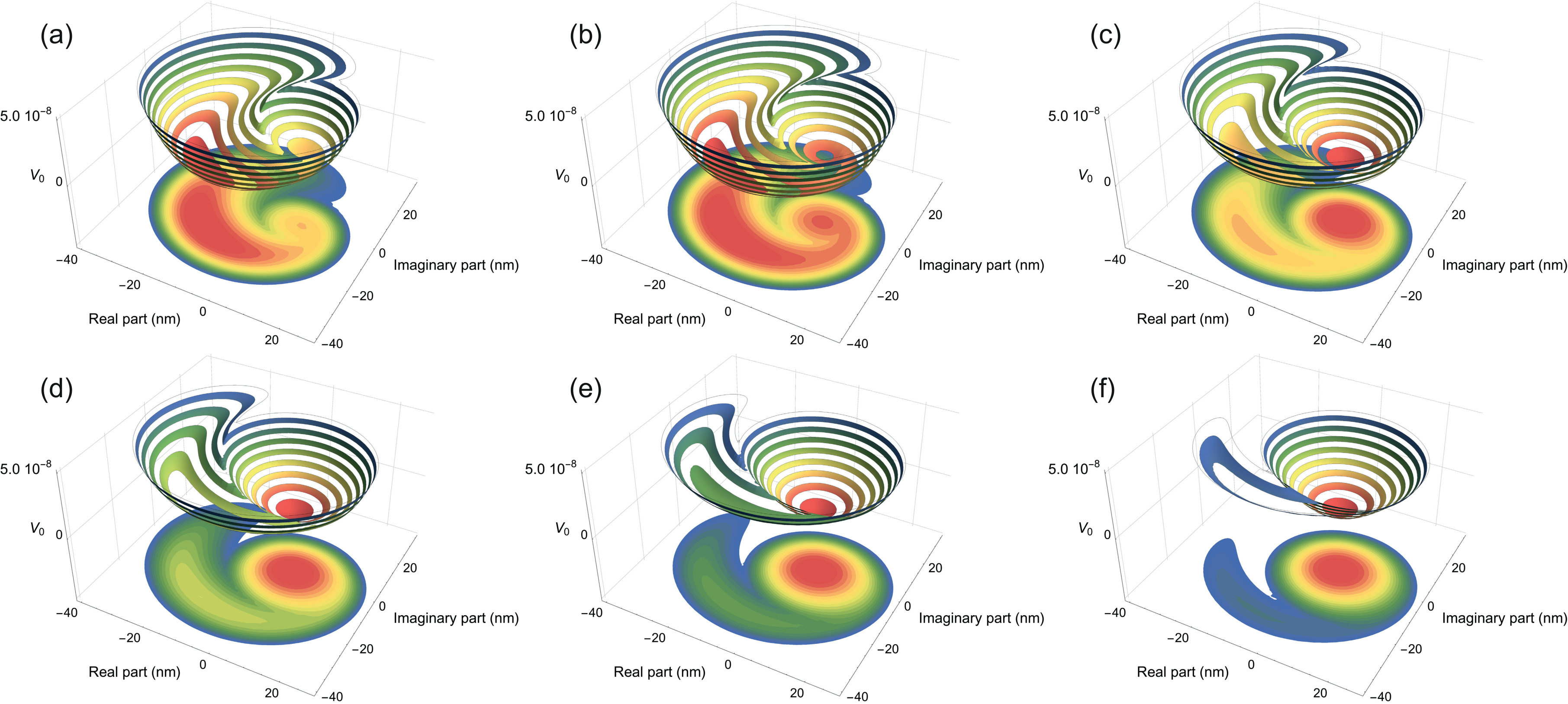 Figure 1
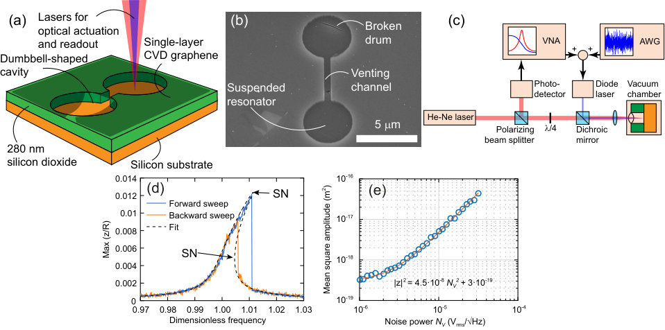 Figure 1
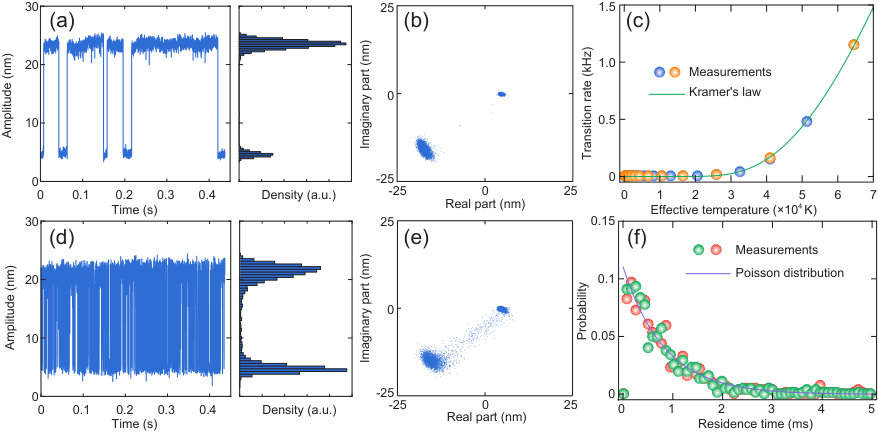 Figure 2
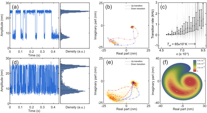 Figure 3
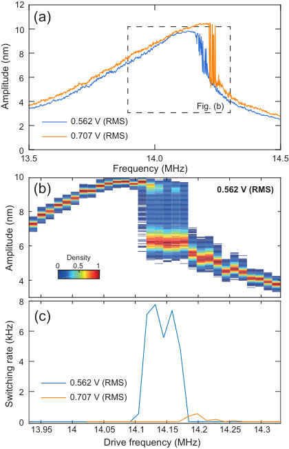 Figure 4
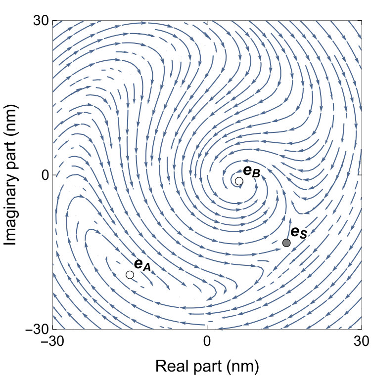 Figure 6
Peer Reviews
No public reviews on file for this paper yet. If you reviewed it on a platform where reviews are public (OpenReview, ICLR, NeurIPS, ICML), you can paste yours below so the community can read it here.
Videos
No videos yet. Explain this paper in a talk, walkthrough, or lecture? Add one.
\useunder
\ul
High-frequency stochastic switching of graphene resonators near room temperature
Robin J. Dolleman
Kavli Institute of Nanoscience, Delft University of Technology, Lorentzweg 1, 2628 CJ, Delft, The Netherlands
Pierpaolo Belardinelli
Department of Precision and Microsystems Engineering, Delft University of Technology, Mekelweg 2, 2628 CD, Delft, The Netherlands
Samer Houri
Kavli Institute of Nanoscience, Delft University of Technology, Lorentzweg 1, 2628 CJ, Delft, The Netherlands
Current affiliation: NTT Basic Research Laboratories, NTT Corporation, 3-1, Morinosato Wakamiya, Atsugi, Kanagawa, 243-0198, Japan
Herre S.J. van der Zant
Kavli Institute of Nanoscience, Delft University of Technology, Lorentzweg 1, 2628 CJ, Delft, The Netherlands
Farbod Alijani
Department of Precision and Microsystems Engineering, Delft University of Technology, Mekelweg 2, 2628 CD, Delft, The Netherlands
Peter G. Steeneken
Kavli Institute of Nanoscience, Delft University of Technology, Lorentzweg 1, 2628 CJ, Delft, The Netherlands
Department of Precision and Microsystems Engineering, Delft University of Technology, Mekelweg 2, 2628 CD, Delft, The Netherlands
Abstract
Stochastic switching between the two bistable states of a strongly driven mechanical resonator enables detection of weak signals based on probability distributions, in a manner that mimics biological systems. However, conventional silicon resonators at the microscale require a large amount of fluctuation power to achieve a switching rate in the order of a few Hertz. Here, we employ graphene membrane resonators of atomic thickness to achieve a stochastic switching rate of 7.8 kHz, which is 200 times faster than current state-of-the-art. The (effective) temperature of the fluctuations is approximately 400 K, which is 3000 times lower than the state-of-the-art. This shows that these membranes are potentially useful to transduce weak signals in the audible frequency domain. Furthermore, we perform numerical simulations to understand the transition dynamics of the resonator and derive simple analytical expressions to investigate the relevant scaling parameters that allow high-frequency, low-temperature stochastic switching to be achieved in mechanical resonators.
Stochastic switching is the process by which a system transitions randomly between two stable states, mediated by the fluctuations in the environment. This phenomenon has been observed in a variety of physical and biological systems Wiesenfeld and Moss (1995); Russell et al. (1999); Longtin et al. (1991); McNamara et al. (1988); Hibbs et al. (1995); Spano et al. (1992); Rouse et al. (1995); Gammaitoni et al. (1998); Lapidus et al. (1999); Hales et al. (2000); Tretiakov and Matveev (2005); Wilkowski et al. (2000); Ricci et al. (2017); Rondin et al. (2017); Levin and Miller (1996); Douglass et al. (1993). Similarly, mechanical resonators that are strongly driven can show stochastic switching between two stable attractors Stambaugh and Chan (2006); Dykman et al. (1998); Chan et al. (2008). This can potentially improve the transduction of small signals in a manner that mimics nature, by the stochastic resonance phenomenon Badzey and Mohanty (2005); Aldridge and Cleland (2005); Chan and Stambaugh (2006); Ono et al. (2008); Venstra et al. (2013). However, high fluctuation power, far above the fluctuations present at room temperature needs to be applied to achieve stochastic switching. Despite the high resonance frequencies achieved by scaling down the resonators to the micro- or nanoscale regime, the switching rate is often quite low, in the order of 1 to 10 Hz. Extending this frequency range to the kHz regime, while lowering the fluctuation power, opens the door for new applications in the audible domain, such as ultra-sensitive microphones.
Mechanical resonators consisting of an atomically thin membrane are ideal candidates to raise the switching rate. Their low mass ensures a MHz resonance frequency that can be easily brought in the nonlinear regime. Graphene is a single layer of carbon atoms with excellent mechanical properties Novoselov et al. (2005); Geim and Novoselov (2007); Lee et al. (2008). Several works have demonstrated graphene resonators Bunch et al. (2007); Chen et al. (2009), showing nonlinear behavior Davidovikj et al. (2017); Dolleman et al. (2018) and several practical applications such as pressure Bunch et al. (2008); Smith et al. (2013); Dolleman et al. (2016); Eichler et al. (2011) and gas sensors Koenig et al. (2012); Dolleman et al. (2017a). The lower mass and low stiffness by virtue of the membranes thinness allows high switching rates to be achieved at lower fluctuation levels.
Here we demonstrate high-frequency stochastic switching in strongly driven single-layer graphene drum resonators. Using an optical drive and readout, we bring the resonator into the bistable regime of the nonlinear Duffing response. By artificially adding random fluctuations to the drive, the effective temperature of the resonator is increased. We observe that the switching rate is increased with an effective temperature dependence that follows Kramer’s law Kramers (1940). Switching rates as high as 7.8 kHz are observed close to room temperature. This work thus demonstrates a stochastic switching frequency that is more than a factor 100 higher than in prior works on mechanical resonators Venstra et al. (2013), at an effective temperature that is over a factor 3000 lower. Having a high stochastic switching rate is important to enable high-bandwidth sensing using this sensitive technique. Moreover, a low effective temperature is relevant to lower power consumption, and if can be brought down to room temperature, the intrinsic Brownian motion of the resonator can be used to enable stochastic switching based sensors. With stochastic switching frequencies above 20 Hz, this work demonstrates the potential of graphene membranes to transduce signals in the audible frequency range.
Fabrication of the samples starts with a silicon chip with a 285 nm thick thermally grown silicon dioxide layer. Dumbbell-shaped cavities as shown in Figs. 1(a) and (b) are etched into the oxide layer using reactive ion etching. Single layer graphene grown by chemical vapor deposition is transferred on top of the sample using a support polymer. This polymer is dissolved and subsequently dried using critical point drying, which results in breaking of one side of the dumbbell and leaves a suspended resonator on the other end that is used for the experiment Dolleman et al. (2017b).
Figure 1(c) shows a schematic representation of the experimental setup used to actuate and detect the motion of single-layer graphene membranes. The red helium-neon laser is used to detect the motion of the membranes and the amplitude of motion is calibrated using nonlinear optical transduction Dolleman et al. (2017c). The blue (405 nm) power-modulated diode laser thermally actuates the movement of the membrane, which can easily reach the bistable geometrically nonlinear regime Dolleman et al. (2017b, 2018). A vector network analyzer (VNA, Rohde and Schwarz ZNB4-K4) actuates the membrane by sweeping the frequency forward and backward and measures the amplitude and phase of the motion. The effective temperature of the resonator is artificially raised using an arbitrary waveform generator (AWG) that outputs white noise.
In order to quantify the effective temperature, the Brownian motion of the device is measured as a function of noise power outputted by the AWG (Fig. 1(e)). From a Lorentzian fit, the mean square amplitude of the device is derived which we use to define the effective temperature Hauer et al. (2013):
[TABLE]
where is the modal mass, the resonance frequency and is Boltzmann’s constant. The effective temperature is a means to express the fluctuation level in an intuitive manner: the fluctuations are identical to the thermal fluctuations of an undriven resonator at an actual temperature of .
Since the amplitude is calibrated, the mean square amplitude at low fluctuation powers (where , being the environmental temperature) can also be used to determine the modal mass of the resonance. From the equipartition theorem Hauer et al. (2013):
[TABLE]
we find 1.85$$ fg. With the known modal mass, we can use the frequency response in Fig. 1(d) to find the equation of motion. By fitting this frequency response we find the dimensionless equation of motion:
[TABLE]
with the damping ratio, corresponding to a quality factor of 833, the cubic stiffness coefficient and 3\text{\times}{10}^{-5}$$. The fundamental frequency of the resonator is 13.92 MHz. The equation uses the generalized coordinate which represents the deflection of the membrane’s center and uses scaled variables to introduce only the relevant combinations of the parameters (see Supporting Information S1).
Before the experiment the resonator is prepared in a bistable state as shown in Fig. 1(d). The frequency is swept forward and backward to reveal the hysteretic behavior of the device and the fixed drive frequency is then set to be in the center between the two saddle-node bifurcations. During the experiment, the amplitude and phase of the resonator are probed as function of time using the VNA. There are now two signal sources driving the system: the fixed driving frequency from the VNA and the random fluctuations provided by the AWG. At a fluctuation power of approximately K the stochastic switching events are observed as shown in Fig. 2(a). The amplitude is split into the in-phase () and out-of-phase () part () as shown in Fig. 2(b), which reveals the two stable configurations of the resonator. Increasing the fluctuation power increases the switching rate as shown in Fig. 2(d) at K. This also causes some broadening of the stable attractors, as can be seen from Fig. 2(e). The experimentally observed switching rate as function of the fluctuation power expressed in is shown in Fig. 2(c). The experiment was repeated twice to check whether effects of slow frequency drift or other instabilities are affecting the experimental result, however both measurements show the same trend. From measurements on other mechanical systems in literature, we expect the switching rate between the stable attractors to follow Kramer’s law Kramers (1940); Gammaitoni et al. (1998); Venstra et al. (2013); Ricci et al. (2017):
[TABLE]
where is the transition rate, is an energy barrier, is the Boltzmann constant and is a parameter used for fitting. Fitting eq. 4 to the experimentally observed transition rate in Fig. 2(b) shows good agreement with the experimental result. From the fit, we obtain an energy barrier of aJ. This energy barrier can be derived from the experimentally obtained amplitudes and effective mass as will be discussed in detail below.
To further investigate the transition dynamics of the system, we plot the residence time distribution of two separate measurements at K as shown in Fig. 2(d). The residence time distribution should follow a Poisson distribution:
[TABLE]
which is used to fit to the experimental data. From the fit, we find that the transition time ms, which corresponds to a transition rate of kHz. This is close to the experimentally obtained value of kHz.
In order to further understand the dynamic behavior of the device, eq. 3 is used to perform numerical simulations of the system in the presence of fluctuations to compare to the experimental results. We analyze the dynamics of the nonlinear oscillator using the method of averaging Kryloff et al. (1947); Dykman et al. (1998). This method describes the change of the vibration amplitude in time by ironing out the fast oscillations (see Supporting Information S1 for further details). Averaging is appropriate since the quality factor is high and the transition rate is much lower than the resonance frequency.
First, a linear stability analysis is performed for the deterministic system. The eigenvalues of the linearized system predicts two stable equilibria separated by an unstable equilibrium (a saddle). The original model is perturbed by adding a Gaussian white noise process, with intensity , details of which are shown in Supporting Information S1. The intensity was matched to the experiments by evaluating the mean square amplitude due to the fluctuations from the simulations and matching them to the experimentally measured mean square amplitude in Fig. 1(b). The stochastic switching behavior obtained via numerical integration of the stochastic differential equations can be seen in Figure 3.
We simulate a time evolution of the system as shown in Fig. 3(a), matching the time and effective temperature of the fluctuations of the experiment in Fig. 2(a). From these simulations, it can be seen that the large amplitude solution is the most probable state for the low-fluctuation configuration because the system resides for most of the time in the basin of attraction of this stable point (see the histogram in Fig. 3(a)). Fig. 3(d), which corresponds to the measurement in Fig. 2(d), shows a massive number of transitions for the resonator with a more equal residence time distribution in the two separate states. The numerical prediction is in qualitative agreement with the switching density illustrated in Figs. 2(a) and (d).
The linear stability analysis of dynamical systems unveils the existence and local properties of a given steady state, but cannot provide information on more complex systems characterized by meta-stable attractors. Moreover, for our system in slow variables the potential function cannot be obtained by integration of the acting forces, thus it results difficult to gain further insights. However, the non-gradient vector field can be decomposed into a gradient term (quasi-potential function) and to its perpendicular constrained remainder (circulatory component). While the latter causes orbits to circulate around energy level sets, the quasi potential gives a 2D surface in which all the trajectories move “downhill” in the absence of perturbations before reaching the steady states, thus satisfying Lyapunov’s global metastability condition Zhou et al. (2012). The quasi-potential function, is calculated by solving the Hamilton-Jacobi equation associated with the equations for and Nolting and Abbott (2016). The fixed points of the deterministic skeleton of the system represent the starting point of the the standard ordered upwind method Sethian and Vladimirsky (2001). Then an expanding front of points is created marching the quasi-potential outward by keeping solutions at adjacent points in ascending order. For the numerical implementation, the free R-package QPot has been adoptedMoore et al. (2015). The quasi-potential gives a qualitative picture of the slow dynamics of the system, with minima near the fixed points of the system as shown in Fig. 3(f).
The probability for the membrane to undergo in large/small harmonic oscillations is related to drive frequency . Indeed, when one solution approaches the saddle, the area of its basin of attraction progressively shrinks whereas the other attractive set conforms as the predominant with the deepest potential well of the system. The evolution of the quasi potential close to the saddle-node bifurcations of the selected bistable region is given in the Supporting Information S2.
Figs. 3(a) and (d) show broad oscillations around the low-amplitude stable equilibrium, while more confined motion is observed around the high-amplitude equilibrium state. The quasi-potential well (top-right Fig. 3(f)) associated with the low-amplitude state has a broader shape allowing for larger deviations from the equilibrium state before the transition. The density diagrams of the solution for the long-term ( s) realization of the system are reported in Fig. 3(b), (c) and (e).
At low-fluctuation levels (Fig. 3(b)) the cloud spread is limited and the switching paths (blue and red paths in Fig. 3(b)) are concentrated in crossing the saddle (gray dot in Fig. 3(f)). The direction of the trajectories is in full accordance with the rotation of the orbits predicted by the stability analysis (Supporting Information S1). Figure 3(e) illustrates a set of paths used by the system to revert its states. Moreover, it shows a larger spread in the phase-space, due to stronger excitation of slow-dynamics around each of the fixed points, besides the higher frequency stochastic switching between low and high-amplitude states. Finally, the switching rate as a function of the intensity of the additive Gaussian noise is reported in Fig. 3(c). For the case of 65\text{\times}{10}^{3}$$ K, corresponding to , the simulated transition rate is kHz, consistent with the experimental findings.
Our experiments show high-frequency stochastic switching at lower effective temperatures. It is interesting to investigate how the system can be engineered to increase the switching rate further, for example to 20 kHz for microphone applications, while reducing the temperature of the fluctuations to room temperature. To reduce the effective temperature, from eq. 4 one needs to reduce the energy barrier . This energy barrier cannot be estimated from the 2D quasipotential used to understand the transition dynamics in the slow-variables. However, a simplified understanding of the dynamics can be used to estimate the value of in Kramers law that applies to a mechanical system. For this, we assume the system undergoes a harmonic motion and neglect the anharmonic part of the motion. The total mechanical energy of a system undergoing harmonic motion with amplitude and frequency , will have a constant total mechanical energy equal to the maximum kinetic energy:
[TABLE]
Now, if a membrane undergoes harmonic oscillation in the low-amplitude attractor with amplitude , it will switch to the other attractor once it reaches amplitude , as it crossed the saddle (Fig. 3(f)). Thus, the work that the thermal fluctuations must do on the system to induce a switch is equal to:
[TABLE]
which is the energy barrier of the low amplitude attractor. For the system oscillating in the high amplitude attractor, work must be performed by the thermal fluctuations in order to reduce the amplitude sufficiently below the saddle amplitude. This means that for the high amplitude attractor we have the energy barrier:
[TABLE]
The switching rate from Kramers law in eq. 4 is now obtained using:
[TABLE]
the energy barrier in eq. 4 is thus given by:
[TABLE]
note that the energy of the saddle has dropped out, and the total energy barrier in Kramer’s law for a bistable Duffing resonator is given by the difference in mechanical energy of the high and low amplitude oscillations. Since we measured and the amplitudes (Fig. 2), we can evaluate eq. 10. We find 3.63$$ aJ, close to the energy barrier of 2.95 aJ obtained from eq. 4. The somewhat lower energy barrier obtained from the experimentally measured switching rate can most likely be attributed to the broadening of the attractors, induced by the fluctuations. This effectively lowers the term in eq. 10 at certain time instances.
Equation 10 gives the relevant parameters that reveal the operating parameters and the properties of the resonator desired to reduce the energy barrier in Kramer’s law, to obtain low-temperature stochastic switching. For this, we assume the bistable region is close to the resonance frequency, and write:
[TABLE]
Two parameters are thus crucial to achieve stochastic switching at low temperatures. First, the effective stiffness should be as low as possible, the ultimate thinness of graphene helps to achieve this. This could be improved further by sculpting the graphene using electron or ion beams Song et al. (2011); Fischbein and Drndić (2008). The second parameter that can be improved is the difference between the amplitudes squared: . This can be achieved by tuning the fixed driving frequency to be closer to the saddle node with the lowest frequency, or by driving the system at lower powers close to the critical forcing amplitude where the resonator becomes unstable. It should be noted that the prefactor in Kramer’s law (Eq. 4) has been left out of this analysis, as it depends on the curvatures of the quasi-potential function and effective damping of the slow dynamics of the system, making it more difficult to predict. However, we expect qualitatively that lowering the amplitude difference also favourably scales the pre-factor , as the curvature of the quasi-potential around the equilibrium points should reduce.
To qualitatively show that minimizing results in stochastic switching at lower temperatures, we perform an additional experiment on a different 3-micron diameter drum in Fig. 4. We drive the system at two different driving levels as shown in Fig. 4(a), 0.562 V is almost above the critical forcing amplitude where the system becomes unstable. At these low driving levels, stochastic swtiching events are readily observed without adding noise to the system. Figure 4(b) shows the histogram of the amplitude at different fixed driving frequencies and Fig. 4(c) shows the corresponding switching rates. Close to the critical force we observe a maximum switching rate of 7762 Hz. The state-of-the-art in conventional MEMS devices achieved a 30 Hz swiching rate at an effective temperature of K Venstra et al. (2013), we have thus improved the switching rate by a factor of 200. For the effective temperature, we have to consider that the laser increases the temperature of the graphene drum somewhat. If we take the total absorbed laser power in the graphene to be roughly 0.1 mW, from measurements on similar sized drums in literature Cai et al. (2010) we estimate the maximum temperature in the drum to be roughly 400 K. The temperature of the fluctuations has thus been lowered by a factor of at least 3000.
In conclusion, we have demonstrated kHz range stochastic switching on graphene drum resonators. The switching rate is two orders of magnitude higher, while the effective temperature of the fluctuations is three orders of magnitude lower than in state-of-the-art MEMS devices. The dynamical behavior and the shape of the cycling paths are qualitatively explained by the shape of the quasi-potential around the two meta-stable equilibria that describes the system’s slow dynamics. Further work can focus on increasing the switching rate and lowering of the fluctuation threshold energy to enable high-bandwidth (>10 kHz), stochastic switching enhanced, sensing at room temperature.
Acknowledgements.
The authors thank Applied Nanolayers B.V. for the supply and transfer of single-layer graphene. We acknowledge Y. M. Blanter for useful discussions. This work is part of the research programme Integrated Graphene Pressure Sensors (IGPS) with project number 13307 which is financed by the Netherlands Organisation for Scientific Research (NWO). The research leading to these results also received funding from the European Union’s Horizon 2020 research and innovation programme under grant agreement No 785219 Graphene Flagship. F.A. acknowledges support from European Research Council (ERC) grant number 802093.
I Supporting information
S1: Equations of motion
I.1 The deterministic skeleton
The dimensionless equation that governs the dynamics of the drum is
[TABLE]
In our formulation the displacement of the membrane’s center is normalized with respect to the membrane radius , i.e. . The time variable is made dimensionless by making use of the resonant frequency . The overdot in eq. (12) means differentiation with respect to the dimensionless time . The amplitude and frequency of the excitation are and , related to their dimensionless counterparts and , respectively. The symbol indicates the effective mass of the drum. The membrane damping is scaled to the dimensionless damping ratio . Finally, is the dimensionless conjugate of the cubic stiffness coeficient .
In order to analyze the slow dynamical evolution of the system, the solution is assumed to have the form
[TABLE]
in which and are slowly varying functions of time. Following the method of variation of parameters, the solution is subject to the condition Kryloff et al. (1947):
[TABLE]
By substituting eq. 13 with its corresponding time derivatives into eq. 12, and making use of eq. 14, we obtain:
[TABLE]
I.2 Stochastic differential system
The deterministic skeleton of the system (Fig. 5) shows 3 equilibria: , and . A linear stability analysis tells us that and are stable equilibrium, whereas is a saddle point. The real part of the eigenvalues of the Jacobian for the stable equilibrium is the same for both the stable equilibrium points ( for , for , and for ) suggesting an equal stability.
The deterministic system of eqs. (15) is then perturbed by a Gaussian white noise process with intensity and in the equations for and , respectively. The system of stochastic differential equations (SDE) with additive noise is:
[TABLE]
in which and are independent Wiener processes, normally distributed random variables with mean zero and variance dt. Note that neither nor the state variables and are anywhere differentiable now that the system is converted to a set of stochastic differential equations. For the integration of eq. 16, the Itô scheme will be employed Oksendal (2013).
S2: Quasi-potential evolution in the bistable region
Here we report the conformation of the quasi potential for different values of the excitation in Eq. (6).
The shape of the quasi-potential surface changes drastically with the drive frequency. In Fig. 6 we show the change of the system from one meta-stable equilibrium to the other. Approaching the membrane resonance through large frequencies (), the low amplitude solution loses progressively its stability increasing the extension of the basin for the high amplitude resonant solution (see Fig. 6(a)). The analysis presented in the main manuscript for realizes an intermediate situation with wells not dissimilar in depth. However, thanks to the quasi-potential, we observe that the well for the low-amplitude solution is more confined and able to trap orbits.
The reference list from the paper itself. Each links out to its DOI / PubMed record.
- 1Wiesenfeld and Moss (1995) Kurt Wiesenfeld and Frank Moss, “Stochastic resonance and the benefits of noise: from ice ages to crayfish and squids,” Nature 373 , 33 (1995).
- 2Russell et al. (1999) David F Russell, Lon A Wilkens, and Frank Moss, “Use of behavioural stochastic resonance by paddle fish for feeding,” Nature 402 , 291 (1999).
- 3Longtin et al. (1991) André Longtin, Adi Bulsara, and Frank Moss, “Time-interval sequences in bistable systems and the noise-induced transmission of information by sensory neurons,” Physical Review Letters 67 , 656 (1991).
- 4Mc Namara et al. (1988) Bruce Mc Namara, Kurt Wiesenfeld, and Rajarshi Roy, “Observation of stochastic resonance in a ring laser,” Physical Review Letters 60 , 2626 (1988).
- 5Hibbs et al. (1995) AD Hibbs, AL Singsaas, EW Jacobs, AR Bulsara, JJ Bekkedahl, and F Moss, “Stochastic resonance in a superconducting loop with a Josephson junction,” Journal of Applied Physics 77 , 2582–2590 (1995).
- 6Spano et al. (1992) ML Spano, M Wun-Fogle, and WL Ditto, “Experimental observation of stochastic resonance in a magnetoelastic ribbon,” Physical Review A 46 , 5253 (1992).
- 7Rouse et al. (1995) R Rouse, Siyuan Han, and JE Lukens, “Flux amplification using stochastic superconducting quantum interference devices,” Applied Physics Letters 66 , 108–110 (1995).
- 8Gammaitoni et al. (1998) Luca Gammaitoni, Peter Hänggi, Peter Jung, and Fabio Marchesoni, “Stochastic resonance,” Reviews of Modern Physics 70 , 223 (1998) . · doi ↗