Topologies of random geometric complexes on Riemannian manifolds in the thermodynamic limit
Antonio Auffinger, Antonio Lerario, Erik Lundberg

TL;DR
This paper studies the topological properties of random geometric complexes on Riemannian manifolds in the thermodynamic limit, establishing universal laws and the convergence of homotopy type distributions.
Contribution
It proves the existence of universal limit laws for the topology of complexes and characterizes the support of the limiting measure in the thermodynamic regime.
Findings
Convergence of normalized homotopy type counts to a deterministic measure
Support of the limiting measure includes all Euclidean homotopy types
Universal laws apply to complexes on Riemannian manifolds
Abstract
We investigate the topologies of random geometric complexes built over random points sampled on Riemannian manifolds in the so-called "thermodynamic" regime. We prove the existence of universal limit laws for the topologies; namely, the random normalized counting measure of connected components (counted according to homotopy type) is shown to converge in probability to a deterministic probability measure. Moreover, we show that the support of the deterministic limiting measure equals the set of all homotopy types for Euclidean geometric complexes of the same dimension as the manifold.
Click any figure to enlarge with its caption.
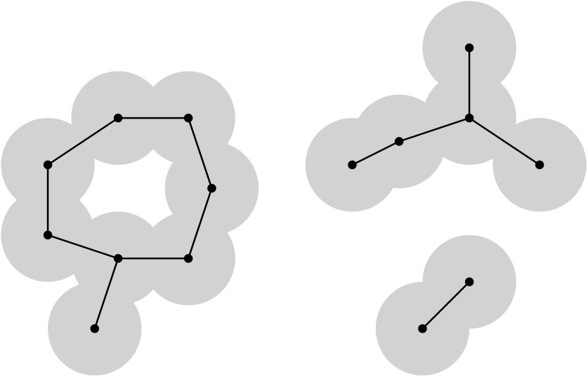 Figure 1
Peer Reviews
No public reviews on file for this paper yet. If you reviewed it on a platform where reviews are public (OpenReview, ICLR, NeurIPS, ICML), you can paste yours below so the community can read it here.
Videos
No videos yet. Explain this paper in a talk, walkthrough, or lecture? Add one.
Topologies of random geometric complexes on Riemannian manifolds
in the thermodynamic limit
Antonio Auffinger, Antonio Lerario, Erik Lundberg
Abstract.
We investigate the topologies of random geometric complexes built over random points sampled on Riemannian manifolds in the so-called “thermodynamic” regime. We prove the existence of universal limit laws for the topologies; namely, the random normalized counting measure of connected components (counted according to homotopy type) is shown to converge in probability to a deterministic probability measure. Moreover, we show that the support of the deterministic limiting measure equals the set of all homotopy types for Euclidean connected geometric complexes of the same dimension as the manifold.
1. Introduction
Sarnak and Wigman [19] recently established, utilizing methods developed by Nazarov and Sodin [15], the existence of universal limit laws for the topologies of nodal sets of random band-limited functions on Riemannian manifolds. In the current paper, we adapt these methods to the setting of random geometric complexes, that is, simplicial complexes with vertices arising from a random point process and faces determined by distances between vertices.
Kahle [13] made the first extensive investigation into the topology of random geometric complexes generated by a point process in Euclidean space (zero-dimensional homology of random geometric graphs were also investigated earlier in [17]). The expectation of each Betti number is studied within three main phases or regimes based on the relation between density of points and radius of the neighborhoods determining the complex: the subcritical regime (or “dust phase”) where there are many connected components with little topology, the critical regime (or “thermodynamic regime”) where topology is the richest (and where the percolation threshold appears), and the supercritical regime where the connectivity threshold appears. The thermodynamic regime is seen to have the most intricate topology. Many cycles of various dimensions begin to form as we enter this regime and many cycles become boundaries as we leave this regime.
Random geometric complexes on Riemannian manifolds were studied earlier in the influential work [16] of Niyogi, Smale, and Weinberger, where the manifold is embedded in Euclidean space and the distance between vertices is given by the ambient Euclidean distance.111 In the current paper, where our manifold is not necessarily embedded, we use geodesic distance to build the complexes. If the manifold happens to be embedded, it can be seen, using Lemma 2.1, that the same limit law stated in Theorem 1.1 holds when using the ambient Euclidean distance. The main question in [16] is motivated by applications in “manifold learning” and concerns the recovery of the topology of a manifold via a random sample of points on the manifold. Consequently, the authors only consider a certain window within the supercritical regime. The subsequent study [5] includes the thermodynamic regime where they provide upper and lower bounds of the same order of growth for each Betti number.
Yogeshwaran, Subag, and Adler [20] established limit laws (including a central limit theorem) in the thermodynamic regime for Betti numbers of random geometric complexes built over Poisson point processes in Euclidean space. More recently, Goel, Trinh, and Tsunoda [11] established a limit law in the thermodynamic regime for Betti numbers of random geometric complexes built over (possibly inhomogeneous) Poisson point processes in Euclidean space, where they also addressed the case when the point process is supported on a submanifold.
Hiraoka, Shirai, and Trinh [12] proved a limit law for so-called “persistent” Betti numbers. Although this goes in a rather separate direction motivated by topological data analysis, the formalism they use for describing the convergence of the persistence diagram has a loose resemblance to the setup of the current paper in that they introduce a sequence of random measures and show that it converges in an appropriate sense to a deterministic measure.
A survey of other results on random geometric complexes is provided in [4]. Most progress in this area has been made only recently, but the problem of studying the topology of a random geometric complex (or equivalently the -neighborhood of a random point cloud) can be traced back to one of Arnold’s problems (see the historical note at the end of the introduction).
A novelty of the current paper is that, whereas previous studies of random geometric complexes have focused on Betti numbers, we consider enumeration of connected components according to homotopy type, a count that provides more refined topological information.
1.1. The Riemannian case
Let be a compact Riemannian manifold of dimension , with normalized volume form . Let be a random set of points independently sampled from the uniform distribution on . We denote by the Riemannian ball222In this paper we adopt the convention that when an object is denoted with a “hat” sign, then it is related to Analogous objects related to Euclidean space will have no “hat”. For example a ball in is denoted by and a ball in by . centered at of radius . We fix a positive number and build the random set:
[TABLE]
We denote by the corresponding Cech complex (which for large enough, is homotopy equivalent to itself, see Lemma 2.1 below).
Let now be the set of equivalence classes of -geometric, connected simplicial complexes, up to homotopy equivalence (observe that this is a countable set). In other words, consists of all the connected simplicial complexes that arise as Cech complexes of some finite family of balls in . Note that different manifolds give rise to different sets . For example, among all -geometric complexes we cannot find complexes with nonzero -th Betti number; but if , such complexes belong to . When we simply denote this set by .
Given as above, we define the random probability measure on :
[TABLE]
where the sum is over all connected components of , denotes the type of (i.e., the equivalence class of all connected complexes homotopy equivalent to ), and denotes the number of connected components.
Remark 1*.*
The next theorem deals with the convergence of the random measure in the limit We endow the set of probability measures on the countable set with the total variation distance:
[TABLE]
In this way is a random variable with values in the metric space . Convergence in probability (which is used in Theorem 1.1 and Theorem 1.3) of a sequence of random variables to a limit means that for every we have
Theorem 1.1**.**
The random measure converges in probability to a universal deterministic probability measure supported on the set of connected -geometric complexes.
The “universal” in the previous statement means that does not depend on the manifold (but it depends on its dimension and on the parameter ).
Remark 2*.*
Since is a proper subset of , the measure does not charge some points in . This is consistent with the findings of [6] where it was shown that an additional factor of is needed in the radii of the balls defining in order to see the so-called “connectivity threshold” where nontrivial -dimensional homology appears.
Remark 3*.*
In the one-dimensional case , the set contains only one element: the class of the point (since any connected geometric complex in is contractible). The case is already more interesting, since in this case where is the wedge of -circles ( is the point). In general the support of is more difficult to describe.
Remark 4*.*
We can write the limiting measure as:
[TABLE]
for some non-negative constants , , which depend on the appearing in (1.1), and satisfy with defined in Proposition 3.1. All of the coefficients are strictly positive by Proposition 3.2.
The following result is related to the positivity of all coefficients . While it is not needed for showing such positivity (which follows from Proposition 3.2), it provides additional information on the prevalence of localized components with prescribed homotopy type throughout the manifold, see Section 6.
Proposition 1.2** (Existence of all topologies).**
Let be a finite geometric complex and . There exist (depending on and but independent of and ) such that for every and for large enough:
[TABLE]
Remark 5*.*
Let us point out an interesting consequence of the previous Proposition 1.2: given a compact, embedded manifold , then for large enough with positive probability the pair is homotopy equivalent to the pair . This follows from the fact that, by [16, Proposition 3.1], one can cover with (possibly many) small Euclidean balls with the inclusion a homotopy equivalence – hence the pair is homotopy equivalent to a pair with a -geometric complex.
1.2. The local model (the Euclidean case)
The proof of Theorem 1.1 for the Riemannian case involves a study of a rescaled version of the problem in a small neighborhood of a given point. Specifically, one can fix and a point and study the asymptotic structure of our random complex in the ball . The random geometric complex that we obtain in the limit can be described as follows.
Let be a set of points sampled from the standard spatial Poisson distribution on and for consider the random set:
[TABLE]
We also define to be the subset of consisting of all the connected components of that are completely contained in the interior of . Note that each is now convex, and, by the Nerve Lemma, is homotopy equivalent to the simplicial complex . The relation between and is described in Theorem 4.1.
Similarly to what we have done above, we define the random probability measure on the set of homotopy types of finite and connected -geometric complexes:
[TABLE]
where the sum is over all connected components of . The following result provides a limit law for .
Theorem 1.3**.**
The family of random measures converges in probability to a deterministic probability measure whose support is all of .
It is important to note that the limiting measure appearing in Theorem 1.3 is the same one appearing in Theorem 1.1 (this explains the statement on the support of the limiting measure in Theorem 1.1).
Besides their positivity, little is known about the coefficients in , and a worthwhile computational problem would be to perform Monte Carlo simulations in order to estimate their numerical values and how they depend on . Concerning dependence on , a direction that has been suggested to us by Matthew Kahle is to study whether the dependence of on exhibits any interesting behavior related to the “percolation threshold” (recalling that our random geometric complex is associated to continuum percolation with disks for which existence of a percolation threshold is known [14]).
While this paper was under review, K. A. Dowling and the third author posted a preprint [10] further adapting these methods to study the limiting homotopy distribution for random cubical complexes associated to Bernoulli site percolation on a cubical grid, where it was shown that the limiting homotopy measure has an exponentially decaying tail for subcritical percolation and a subexponential tail (slower than exponential decay) for supercritical percolation. It is then natural to pose a specific version of the above problem suggested by M. Kahle, namely, to investigate the tail decay of in the current setting of random geometric graphs and to determine whether it exhibits a phase transition at the percolation threshold (see [10, Concluding Remarks]).
Outline of the paper. We prove Theorem 1.3 addressing the Euclidean setting in Section 3. In Section 4, we establish the “semi-local” result involving a double-scaling limit within a neighborhood on the manifold, and in Section 5 we collect the semi-local information throughout the manifold in order to prove the global result Theorem 1.1 for the manifold setting. We prove Proposition 1.2 in Section 6. Section 2 contains some basic tools used throughout the paper, including the integral geometry sandwiches that play an essential role.
Historical Note. The study of the topology of random simplicial complexes has taken shape only recently with intense activity in the past few years, but it is worth mentioning (as it seems to have been forgotten) that this theme was proposed by V.I. Arnold in the early 1970s, with specific attention given to random geometric complexes in the thermodynamic regime. In the collection [1] of Arnold’s problems, the 28th problem from 1973 states (notice that the set considered is homotopy equivalent to a geometric complex by the nerve lemma):
Consider a random set of points in with density . Let be the -neighborhood of this set. Consider the averaged Betti numbers
[TABLE]
Investigate these numbers.
Acknowledgements
This work was initiated during the conference “Stochastic Topology and Thermodynamic Limits” that was hosted at ICERM, and part of the work was completed during a second week-long visit to ICERM through the collaborate@ICERM program. The authors wish to thank the institute for their support and for a pleasant and hospitable work environment. The authors would also like to thank the anonymous referee for a careful reading of the paper and many helpful comments regarding the exposition. This research was conducted while A.A. was supported by NSF Grant CAREER DMS-1653552.
2. Preliminary material
In this section we collect some basic tools used throughout the paper.
2.1. Geometry
A subset of a Riemannian manifold is called strongly convex if for any pair of points there exists a unique minimizing geodesic joining these two points such that its interior is entirely contained in (see [7, 9]).
Lemma 2.1**.**
Let be a compact Riemannian manifold. There exists such that for every point and every the ball is strongly convex and contractible. Moreover for every and the set is also strongly convex and contractible. In particular, by the Nerve Lemma, the set is homotopy equivalent to its associated Cech complex.
Proof.
By [7, Theorem 5.14] there exists a positive and continuous function such that if , then is strictly convex (this is in fact due to Whitehead). Since is compact, then . Any strongly convex set in a Riemannian manifold is contractible with respect to any of its point (star-shaped in exponential coordinates), hence it follows that for the ball is also contractible. To finish the proof, we simply observe that the intersection of strongly convex sets is still strongly convex: in fact given two points , by strong convexity of the sets, the unique minimizing geodesic joining the two points is contained in both sets. ∎
From now on, the notation denotes the collection of all -element subsets of
We will say that a -geometric complex is nondegenerate if for every and the intersection is transversal (in particular this intersection is empty for ).
Random geometric complexes are nondegenerate with probability one. However, it could be that without the nondegeneracy assumption one could construct a geometric complex which is not homotopy equivalent to any nondgenerate one. This is not the case, as next Lemma shows.
Lemma 2.2**.**
The set of homotopy types of -geometric, connected, nondegenerate complexes coincides with 333Recall that we did not assume the nondegeneracy condition in the definition of ..
Proof.
Given a possibly degenerate , let be the semialgebraic and continuous function defined by
[TABLE]
and observe that:
[TABLE]
We consider now the semialgebraic, monotone family . By [2, Lemma 16.17] for the inclusion is a homotopy equivalence. It suffices therefore to show that for small enough is nondegenerate; this follows from the fact that given points , for every and there are only finitely many such that the intersection is nontransversal (and the number of possible multi-indices to consider is also finite). ∎
The following Proposition plays an important role in all asymptotic stability arguments.
Proposition 2.3**.**
Let be a compact Riemannian manifold of dimension and . Let be a nondegenerate complex such that:
[TABLE]
for some points and . Given set and consider the sequence of maps:
[TABLE]
Denoting by the inverse of , there exist and such that if for every then for we have:
[TABLE]
Proof.
For and for every either one of these possibilities can verify:
- (1)
, in which case, by nondegeneracy, there exists and such that for all ; 2. (2)
, in which case there is no solving for all .
Since the sequence of maps defined by
[TABLE]
converges uniformly to , then for every there exists such that for all pairs of points and for all we have:
[TABLE]
For every index set satisfying condition (1) above, choosing and setting , the previous inequality (2.7) implies that, if for every , then for :
[TABLE]
This means that the combinatorics of the covers and are the same if for and .
Let us consider now an index set satisfying condition (2) above. We want to prove that there exists and such that if for all , then for the intersection is still empty. We argue by contradiction and assume there exist a sequence of points and for points with such that for all and all large enough:
[TABLE]
We call and assume that (up to subsequences) it converges to some . Using again the uniform convergence of to , the inequality (2.9) would give:
[TABLE]
which gives the contradiction .
Set now and . We have proved that, if for all , then for all the two open covers and have the same combinatorics. In particular their Cech complex is the same. Moreover, Lemma 2.1 implies that for a possibly larger all the balls are strictly convex in ; consequently, by the Nerve Lemma, for larger than such these two open covers are each one homotopy equivalent to their Cech complexes, hence they are themselves homotopy equivalent. ∎
2.2. Measure theory
The following lemma will be used in the proof of Theorem 1.3. This lemma and its proof are essentially in [19, Thm. 4.2 (2)], but we provide a proof to make the paper more self-contained and to ensure that it is clear this result is purely measure-theoretic.
Lemma 2.4**.**
Let be a one-parameter family of random probability measures on , and let be a deterministic probability measure on . Assume that for every in probability as . Then in probability, i.e., for every we have
[TABLE]
where denotes the total variation distance.
Proof.
Let be arbitrary.
Since is a probability measure on , there exists such that
[TABLE]
We have
[TABLE]
which implies (by a union bound)
[TABLE]
and also (by the triangle inequality)
[TABLE]
for .
The estimate (2.13) implies an estimate for the tails:
[TABLE]
since
[TABLE]
which follows from and being probability measures.
For any , we then have
[TABLE]
Indeed, if
[TABLE]
then equation (2.11) gives
[TABLE]
and (2.15) then follows from (2.14).
In order to estimate the total variation distance between and , let be arbitrary. We have:
[TABLE]
Using a union bound, this implies
[TABLE]
which is less than by (2.12) and (2.15).
This implies that for every we have, for all sufficiently large,
[TABLE]
i.e. we have shown
[TABLE]
∎
2.3. The ergodic theorem
The proof of Proposition 3.1 uses the following special case of the -dimensional ergodic theorem. We follow [14, Ch. 2] and [8, Sec. 12.2]).
Theorem 2.5** (Ergodic Theorem).**
Let be a probability space, and let , be an -action on . Let , and suppose further that the action of on is ergodic. Then we have
[TABLE]
as .
Let us explain the terminology appearing in the statement of this theorem. An -action , is a group of invertible, commuting, measure-preserving transformations acting measurably on a probability space and indexed by . An -action is said to be ergodic if any invariant event has probability either zero or one.
For our application of the ergodic theorem (see the proof of Proposition 3.1 below), the -action will simply be translation by acting on the Poisson process (this case is known to be ergodic [14, Prop. 2.6]).
2.4. Component counting function and the integral geometry sandwiches
Definition 1** (Component counting function).**
Let and be topological spaces (in the case of our interest they will be homotopy equivalent to finite simplicial complexes). We denote by the number of connected components of entirely contained in the interior of and which have the same homotopy type as . Similarly, we denote by the number of connected components of which intersect and which have the same homotopy type as .
Theorem 2.6** (Integral Geometry Sandwich).**
Let be a generic geometric complex in and fix . Then for
[TABLE]
Theorem 2.7** (Integral Geometry Sandwich on a Riemannian manifold).**
Let be a generic geometric complex on and fix . Then for any there exists such that for every
[TABLE]
where still denotes the Euclidean ball of radius .
Proofs of Theorems 2.6 and 2.7.
These results follow from the same proof as in [19]. ∎
Remark 6*.*
Similar statements hold true if we take the sum over all components, ignoring their type (an observation used throughout the paper). More precisely, denoting by the number of components of entirely contained in the interior of and by the number of components of that intersect , we have the following inequality:
[TABLE]
and, in the Riemannian framework:
[TABLE]
Since both and have only finitely many components, these inequalities follow by simply summing up the two inequalities from the previous theorems over all components type (the sums are over finitely many elements). In fact the integral geometry sandwiches as proved in [19] are adaptations of the original construction from [15], where components were counted without regard to topological type.
3. Limit law for the Euclidean case
In this section we prove Theorem 1.3. The main step is provided by the following proposition. We continue to use the above notation for the component counting function (see Definition 1).
Proposition 3.1**.**
For every homotopy type there exists a constant such that the random variable
[TABLE]
converges to a constant in as . The same is true for the random variable
[TABLE]
(i.e. when we consider all components, with no restriction on their types): as , it converges to a constant in .
The next proposition is proved in Section 6.
Proposition 3.2**.**
The constants defined in Proposition 3.1 are positive for all .
Proof of Proposition 3.1.
The proof follows the argument from [19, Theorem 3.3], with some needed modifications.
We will use the shortened notation , and ( will be fixed for the rest of the proof and we omit dependence on it in the notation). Using Theorem 2.6 we can write, for :
[TABLE]
Denoting by the annulus , we can estimate the integral on the r.h.s. of (3.3) with:
[TABLE]
In fact, if a component of is not entirely contained in the interior of , then it touches the boundary of and hence this component must contain a point .
We now take (with fixed) and use the Ergodic Theorem in order to assert that
[TABLE]
as where is a constant.
In order to apply the ergodic theorem (Theorem 2.5 stated above) we introduce the function defined as
[TABLE]
where is fixed, and the dependence of on the Poisson process is through which we recall is the -neighborhood of . We also let denote translation by acting on the Poisson process . This action is ergodic as noted above in Section 2. We also have , since
[TABLE]
so that the ergodic theorem may be applied.
Furthermore, we notice that
[TABLE]
i.e., shifting has the same effect as recentering the ball to . Thus, the result of applying the ergodic theorem to this choice of gives precisely the convergence statement in (3.5).
Note that the same convergence statement in (3.5) holds for , namely,
[TABLE]
as where is the same constant as in (3.5).
We also have
[TABLE]
as where . This follows from the ergodic theorem as well (although it seems more natural to view it as a consequence of the law of large numbers).
Let be arbitrary. Since we can choose sufficiently large that . We then choose sufficiently large so that , . Using the above convergence statements (3.5), (3.6), and (3.7) (while making even larger if necessary) we have,
[TABLE]
Using and also that for all , which follows from
[TABLE]
(3.8) implies
[TABLE]
Since was arbitrary, this implies the existence of a constant such that in as and in as .
The proof of the second statement in the proposition concerning the existence of a limit for all components (with no restriction on homotopy type) follows from the same argument while replacing the integral geometry sandwich with its more basic version (see Remark 6 in Section 2). ∎
3.1. Proof of Theorem 1.3
We write the measure as:
[TABLE]
By the convergence statements in Proposition 3.1, and since (which follows from Proposition 3.2 since ), we have converges in to a constant as .
The positivity of the coefficients follows from the positivity of stated in Proposition 3.2.
Next we prove that the measure
[TABLE]
is indeed a probability measure (see Proposition 3.4 below). The main obstacle, addressed in the following lemma (cf. [19, Sec. 4]), is in preventing the mass in the sequence of measures from escaping to infinity.
Lemma 3.3** (Topology does not leak to infinity).**
For every there exists a finite set and such that for all
[TABLE]
Proof of Lemma 3.3.
First we observe that
[TABLE]
where is independent of . Indeed,
[TABLE]
which is a constant independent of (the average number of points of a Poisson process in a given region is proportional to the volume of the region).
Let be arbitrary. Then, using the Integral Geometry Sandwich, we obtain:
[TABLE]
Let be arbitrary, and choose sufficiently large that the above error term is smaller than .
By the convergence (3.12) there exists a finite set such that
[TABLE]
Choosing large enough that we then have for all
[TABLE]
as desired, and this completes the proof of the lemma. ∎
Proposition 3.4**.**
The measure
[TABLE]
with , is a probability measure.
Proof of Proposition 3.4.
We need to show that , or equivalently,
[TABLE]
Let and take to be the set guaranteed by Lemma 3.3.
We want to show that
[TABLE]
which will then immediately establish (3.16) since is arbitrary.
For fixed in the sample space observe that by Fatou’s lemma
[TABLE]
and applying Fatou’s lemma again followed by Tonelli’s theorem, we have
[TABLE]
Combining this with Lemma 3.3 we obtain
[TABLE]
We proceed to estimate :
[TABLE]
In the last line, we have estimated the first and last terms by by choosing sufficiently large and using the convergence (and the fact that is a finite set) and the convergence ; we have estimated the second term by using (3.21); and we have estimated the third term by by choosing sufficiently large to apply Lemma 3.3. This establishes (3.17) and concludes the proof of the proposition. ∎
Having established by Proposition 3.4 that is a probability measure, the convergence in probability now follows from the coefficient-wise convergence along with the purely measure-theoretic result Lemma 2.4.
The statement that the support of is all of follows from the positivity of the coefficients . This concludes the proof of Theorem 1.3.
4. Semi-local counts in the Riemannian case
In this section, we study the components of contained in a neighborhood of a point by relating this case to the Euclidean case. As a preliminary step, we consider the following diffeomorphism (see also Proposition 2.3):
[TABLE]
Through , the stochastic point process induces a stochastic point process on which converges in distribution to the uniform Poisson process on [18, Sec. 3.5]. By Skorokhod’s representation theorem [3, Ch. 1, Sec. 6], there exists a representation, or “coupling”, of these point processes defined on a common probability space such that the convergence of these stochastic processes is almost sure.
Theorem 4.1**.**
Let . For every and for sufficiently large there exists such that (using the coupling given by Skorokhod’s theorem mentioned above) for every and for :
[TABLE]
Proof.
Let denote the inverse of the map defined in (4.1). For the proof of (4.2) we will need to establish the following three facts:
- (1)
There exists and such that with probability at least we have:
[TABLE]
(i.e. with positive probability for large , depending on , both point processes have the same number of points and this number is bounded by some constant , which also depends on ). 2. (2)
There exists444The symbol denotes the disjoint union of the sets . , and such that and for every if is such that and then:
[TABLE]
(i.e. the two spaces are homotopy equivalent), and for every connected component of this component intersects if and only if the corresponding component of intersects
Let us explain this condition. A point in corresponds to the spatial Poisson event: we sample points and each of these points is sampled uniformly from . With probability at least , by the previous point, the number of samples of the spatial Poisson distribution is at most Each such Poisson sample in gives rise to a geometric complex in , and this complex is nondgenerate with probability one. Given such a nondegenerate complex in , we can perturb “a little” (how little is quantified by “”) the point to a point inside and still get a nondegenerate complex which has the same homotopy type of the original one. Now, to each point there also corresponds a complex in the manifold , through the map . When is “large enough”, it is natural to expect that the two complexes and have the same homotopy type. Point (2) says that, given , we can find with probability at least , small enough and large enough such that this is true. (We also added the requirement that the intersection with the boundary of the big containing ball is the same, but the essence of point (2) is in the requirement that the two complexes should have the same homotopy type.) 3. (3)
Assuming point (1), denoting by , and by , there exists such that for every :
[TABLE]
Assuming these three facts, (4.2) follows arguing as follows. With probability at least for all the conditions from (1), (2) and (3) verify and the two random sets
[TABLE]
are homotopy equivalent and by the second part of point (2) also the unions of all the components entirely contained in (respectively ) are homotopy equivalent. In particular the number of components of a given homotopy type is the same for both sets with probability at least .
It remains to prove (1), (2) and (3).
Point (1) follows from the fact that (working with the representation provided by Skorokhod’s theorem), the point process converges almost surely to the Poisson point process on . In particular the sequence of random variables converges almost surely to and (4.3) follows from the fact that almost sure convergence implies convergence in probability.
For point (2) we argue as follows. Given we consider the compact semialgebraic set:
[TABLE]
This set is endowed with the measure :
[TABLE]
where denotes the Lebesgue measure (this is the measure induced from the Poisson distribution).
Let now be the set of points such that either the intersection or the intersection is non-transversal for some index sets (note that the generic intersection of more than spheres will be empty). This set is also a semialgebraic set, and it has measure zero: it cannot contain any open set, because the nondegeneracy condition is open and dense.
Let be an open neighborhood of such that (for example one can take for small enough). We set (note that ).
We will first argue that for every we can find and such that the two complexes (4.4) have the same homotopy type (and the same combinatorics of intersection with the boundary of the big containing ball) whenever and Then we will use the compactness of in order to find uniform and
Pick therefore . The property of transversal intersection implies that for every index set such that the intersection is nonempty, this intersection contains a nonempty open set, and there exists a point such that for every we have Similarly for every whenever an intersection is transversal and nonempty, there exists a point such that and for every we have Because these are open properties, there exists such that for every and with and for all , we have:
[TABLE]
Moreover since the property of having non-empty intersection is also stable under small perturbations, we can assume that are small enough to guarantee also that:
[TABLE]
Observe now that the sequence of functions defined by:
[TABLE]
converges uniformly to the Euclidean distance in . In particular there exists such that for every , for every and with and , for all and for we have:
[TABLE]
Moreover, for a possibly larger , we also have that
[TABLE]
Choosing to be even larger, so that balls of radius smaller than in are geodesically convex, these conditions imply that the combinatorics of the covers
[TABLE]
are the same and, by Lemma 2.1, the two sets and are homotopy equivalent. Also, the above condition on implies that a component of intersects if and only if the corresponding component of intersects
Finally, we cover now with the family of open sets and find, by compactness of , finitely many points such that the union of the balls with covers . With the choice and property (2) is true.
Concerning point (3), we observe that again this follows from the fact that the point process converges almost surely (hence in probability) to the Poisson point process on . ∎
Corollary 4.2**.**
For each , , , and , we have
[TABLE]
Proof.
This follows from Theorem 4.1 combined with Proposition 3.1. Indeed, let and be arbitrary. By Proposition 3.1 there exists such that for we have
[TABLE]
Fix any such . The event
[TABLE]
is contained in the union of the event that
[TABLE]
and another event , which is the event that . Thus,
[TABLE]
By Theorem 4.1, there exists such that for all we have .
Thus, applying this to (4.18) we obtain
[TABLE]
Since was arbitrary, this completes the proof of Corollary 4.2. ∎
5. The global count for the Riemmanian case:
proof of Theorem 1.1
In this section we establish the limit law in the manifold setting (cf. [19, Sec. 7]). As in the Euclidean case, the main step is to prove coefficient-wise convergence, which is stated in the following theorem.
Theorem 5.1**.**
For every , the random variable
[TABLE]
converges in to the constant (the same constant as in Proposition 3.1). The same statement is true for the random variable
[TABLE]
(i.e. when we consider all components, with no restriction on their type): as , it converges in to the constant .
5.1. Proof of Theorem 1.1 assuming Theorem 5.1
Since convergence in implies convergence in probability, Theorem 5.1 ensures that the random variable converges in probability to the constant ; similarly the random variable converges in (hence in probability) to . The proof now proceeds similarly to the proof of Theorem 1.3. We write the measure as:
[TABLE]
We have converges in to the constant . Recalling that the measure
[TABLE]
is a probability measure (see Proposition 3.4), we can apply Lemma 2.4 to conclude that the measure on the left in (5.7) converges in probability to .
Since is a probability measure, this implies that
[TABLE]
converges to in probability. For any this implies that the coefficient appearing in the measure on the right in (5.7) converges to zero in probability, since
[TABLE]
Thus, the measure converges in probability to by another application of Lemma 2.4.
5.2. Proof of Theorem 5.1
Note: Since and are fixed, we will simply use
[TABLE]
to denote the number of components of in of type . We will use
[TABLE]
to denote the number of such components intersecting the geodesic ball of radius centered at and
[TABLE]
to denote the number of components completely contained in .
Thus, our goal, stated in the abbreviated notation (5.8), is to prove
[TABLE]
Using the integral geometry sandwich from Theorem 2.7 we have
[TABLE]
Letting denote the integral on the left side and the one on the right side, we subtract from each part of (5.10) and write
[TABLE]
In order to estimate we note that the number of connected components of that intersect, but are not completely contained in, the geodesic ball is bounded above by the number of points that fall within distance to the boundary . This -neighborhood of is the same as the geodesic annulus centered at with inner radius and outer radius . The average number of points in this annulus equals its volume which can be estimated (uniformly over ) by that of the Euclidean annulus, and this gives
[TABLE]
which together with (5.11) implies
[TABLE]
where we have also used which follows from the first inequality in (5.10) along with the simple estimate .
By (5.13) we obtain
[TABLE]
Thus, in order to prove the theorem it suffices to show that the above term can be made arbitrarily small for all sufficiently large .
Define the “bad” event
[TABLE]
Claim: There exists a sequence such that for every there exists with such that
[TABLE]
The proof of this claim closely follows [19] and uses Egorov’s theorem as well as the idea from the proof of Egorov’s theorem. We start by recalling the point-wise limit stated in Corollary 4.2. For each , we have
[TABLE]
Let us restrict to . Apply Egorov’s theorem to obtain with such that
[TABLE]
Next we use an additional Egorov-type argument in order to obtain the statement in the claim (where we will obtain the set by slightly shrinking ). For each fixed integer , we can find by (5.18) an sufficiently large so that
[TABLE]
Letting denote the monotone decreasing (with ) sequence of sets
[TABLE]
we see from (5.19) that
[TABLE]
Thus, there exists such that . We take
[TABLE]
which satisfies . It follows from the definition of that
[TABLE]
and we see that (5.17) is satisfied.
Denoting the whole probability space as , we separate the integration (defining the expectation) over the two sets and .
[TABLE]
We use the definition of to estimate the first integral in (5.21):
[TABLE]
For the second integral in (5.21), we use the estimate
[TABLE]
where is the minimum (over ) volume of a geodesic ball of radius , which is uniformly (over ) comparable to the volume of the Euclidean ball of the same radius, and hence is bounded below by a constant times . The estimate (5.23) is based on the fact that each component has volume trivially at least a constant times , and the fact that the minimal volume of a component times the number of components cannot exceed the volume of the region where they are contained (while fixing attention on components of type as we are throughout the proof). Applying (5.23), we obtain
[TABLE]
Next, we split this last integration over and :
[TABLE]
Bringing the estimates (5.21), (5.22), (5.24), (5.27) together, we have
[TABLE]
which can be made arbitrarily small using (5.17). This establishes (5.9) and completes the proof of the first part of Theorem 5.1. The proof of the second part concerning the count for all components (without restriction on homotopy type) follows from the same proof while replacing the integral geometry sandwich with its more basic version (see Remark 6 in Section 2).
6. Positivity of all coefficients
In this section, we prove Propositions 3.2 and 1.2.
6.1. Proof of Proposition 3.2
Recall that, by Proposition 3.1, for every we have:
[TABLE]
The desired lower bound will come from adding up certain local contributions provided by the following lemma
Lemma 6.1**.**
Let be a finite geometric complex. Fix . There exist (depending on and ) such that for any
[TABLE]
Proof of Lemma 6.1.
By the translation invariance of the Poisson point process, it is enough to prove the statement while taking . We can assume, by Remark 2.2 above, that is nondegenerate, and we write
[TABLE]
where , and we have taken the radius to be , since we can dilate the entire set if necessary (which does not change the homotopy type). Choose such that . By nondegeneracy, there exists such that if then the two complexes and are homotopy equivalent.
We are thus interested in the event that for each ball contains exactly one point from the random set and that these points are the only points of in the ball . If occurs then we have as desired. The positivity of the probability of the event can be seen by noticing that this probability is a product of finitely many positive probabilities. Indeed, is an intersection of the events that contains a single point from for along with the event that there are no points in the set These events are independent by a basic property of the Poisson point process, and each of them has positive probability (the probabilities can be specified explicitly in terms of the volumes of the sets involved). ∎
Let be given by Lemma 6.1 for the choice of . For an appropriate we can fit many disjoint Riemannian balls
[TABLE]
in . Observing that
[TABLE]
we have (also using linearity of expectation)
[TABLE]
and the positivity of follows.
6.2. Proof of Proposition 1.2
The positivity of coefficients in Theorem 1.1 is already established in Proposition 3.2 proved above. In this section, we prove the related Proposition 1.2 which provides a more direct analysis in the manifold setting.
Proof.
Let and such that
[TABLE]
with a nondegenerate complex (it is not restrictive to consider nondegenerate complexes by Remark 2.2 above). Let now such that contains and set Consider also the sequence of maps:
[TABLE]
Proposition 2.3 implies that there exists and such that if then for the two complexes and are homotopy equivalent.
We are interested in the the event:
[TABLE]
Observe that if verifies, then : in fact, since there is no other point in other than , then the complex is the disjoint union of the two complexes and ; the complex by Proposition 2.3.
It is therefore enough to estimate from below the probability of . Note that for every measurable subset there exists a constant such that . In particular, using the independence of the points in , we can estimate
[TABLE]
In particular there exists such that:
[TABLE]
and this concludes the proof. ∎
The reference list from the paper itself. Each links out to its DOI / PubMed record.
- 1[1] V. I. Arnold. Arnold’s problems . Springer-Verlag, Berlin; PHASIS, Moscow, 2004. Translated and revised edition of the 2000 Russian original, With a preface by V. Philippov, A. Yakivchik and M. Peters.
- 2[2] S. Basu, R. Pollack, and M.-F. Roy. Algorithms in real algebraic geometry , volume 10 of Algorithms and Computation in Mathematics . Springer-Verlag, Berlin, second edition, 2006.
- 3[3] P. Billingsley. Convergence of probability measures . Wiley Series in Probability and Statistics: Probability and Statistics. John Wiley & Sons, Inc., New York, second edition, 1999. A Wiley-Interscience Publication.
- 4[4] O. Bobrowski and M. Kahle. Topology of random geometric complexes: a survey. J. Appl. Comput. Topol. , 1(3):331–364, Jun 2018.
- 5[5] O. Bobrowski and S. Mukherjee. The topology of probability distributions on manifolds. Probab. Theory Related Fields , 161(3-4):651–686, 2015.
- 6[6] O. Bobrowski and S. Weinberger. On the vanishing of homology in random Čech complexes. Random Structures Algorithms , 51(1):14–51, 2017.
- 7[7] J. Cheeger and D. G. Ebin. Comparison theorems in Riemannian geometry . AMS Chelsea Publishing, Providence, RI, 2008. Revised reprint of the 1975 original.
- 8[8] D. J. Daley and D. Vere-Jones. An introduction to the theory of point processes. Vol. II . Probability and its Applications (New York). Springer, New York, second edition, 2008. General theory and structure.