Dynamics and computation in mixed networks containing neurons that accelerate towards spiking
Paul Manz, Sven Goedeke, Raoul-Martin Memmesheimer

TL;DR
This paper explores how neuron diversity, specifically neurons that accelerate towards spiking, influences the dynamics, chaos, and computational abilities of mixed spiking neural networks, revealing that even a single different neuron type can significantly alter network behavior.
Contribution
It introduces a mixed network model with inhibitory LIF and XIF neurons, analyzing their dynamics, stability, and computational potential, highlighting the impact of neuron diversity on network function.
Findings
A single XIF neuron induces chaos in the network.
The network can generate balanced irregular spiking activity.
Different stability properties enable diverse computational capabilities.
Abstract
Networks in the brain consist of different types of neurons. Here we investigate the influence of neuron diversity on the dynamics, phase space structure and computational capabilities of spiking neural networks. We find that already a single neuron of a different type can qualitatively change the network dynamics and that mixed networks may combine the computational capabilities of ones with a single neuron type. We study inhibitory networks of concave leaky (LIF) and convex "anti-leaky" (XIF) integrate-and-fire neurons that generalize irregularly spiking non-chaotic LIF neuron networks. Endowed with simple conductance-based synapses for XIF neurons, our networks can generate a balanced state of irregular asynchronous spiking as well. We determine the voltage probability distributions and self-consistent firing rates assuming Poisson input with finite size spike impacts. Further, we…
Click any figure to enlarge with its caption.
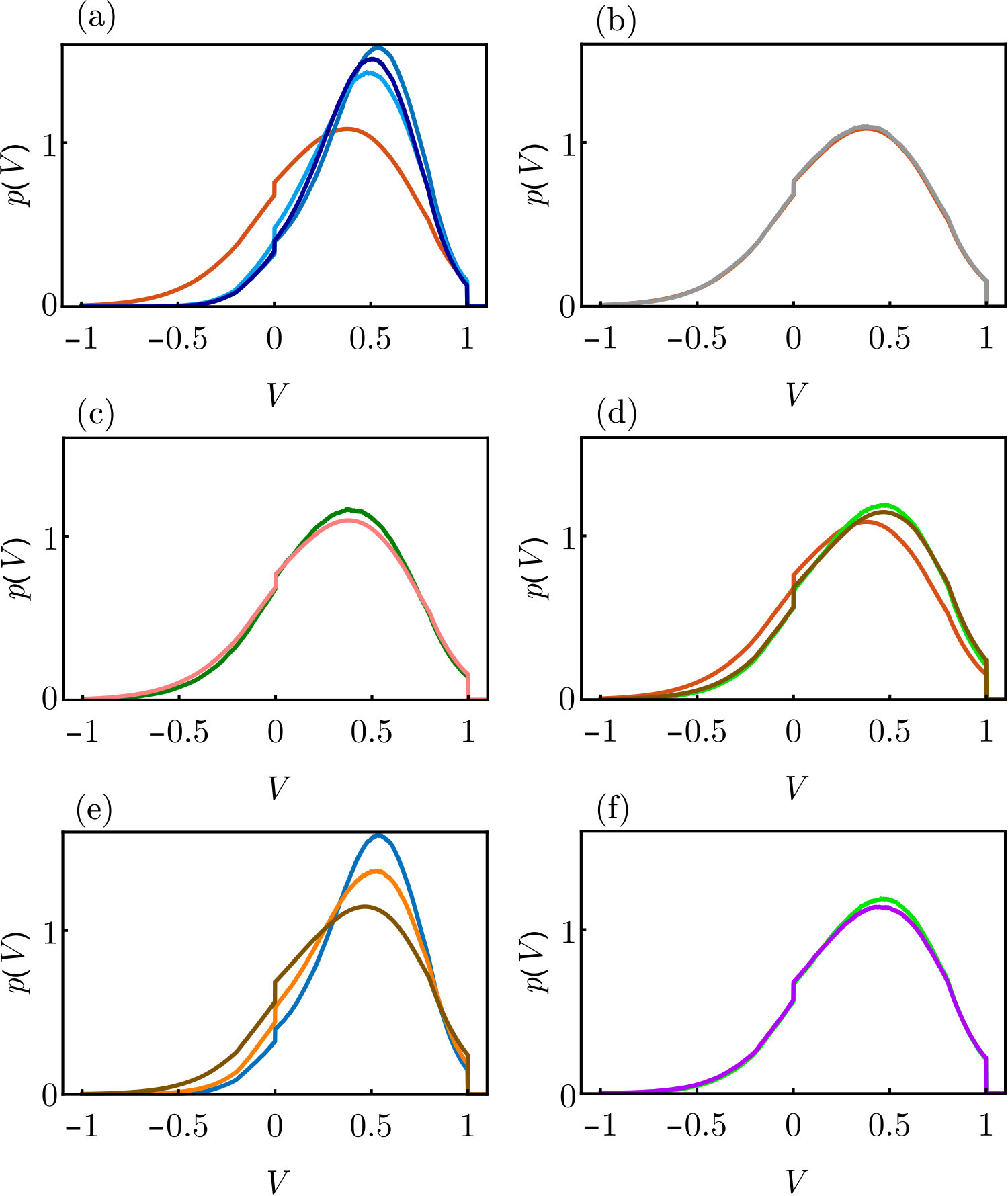 Figure 10
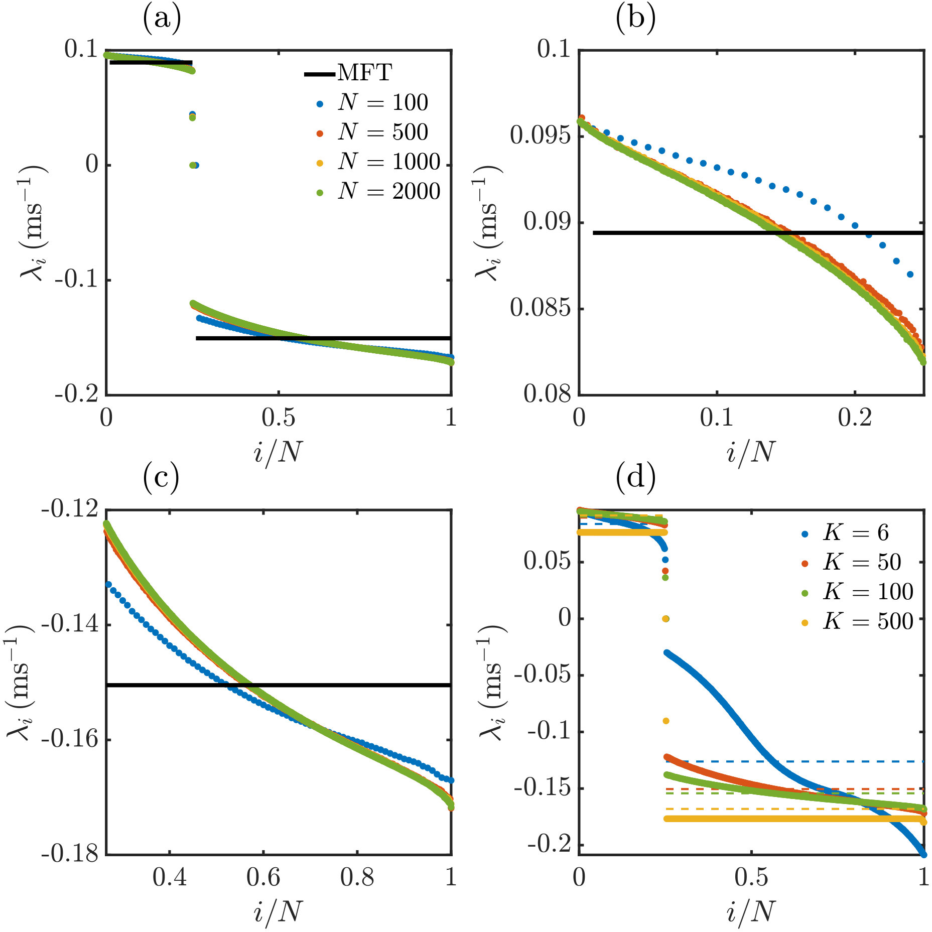 Figure 11
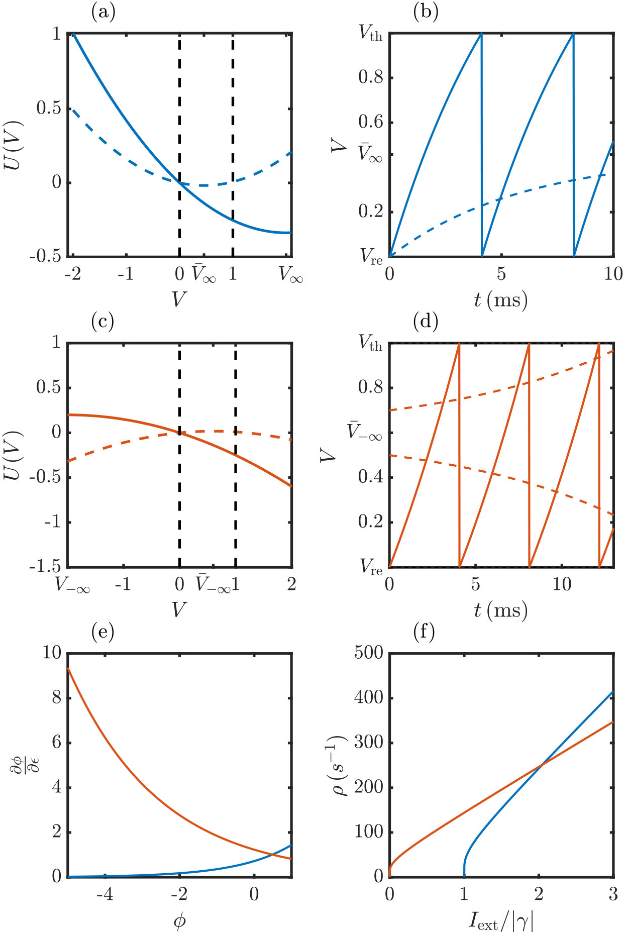 Figure 1
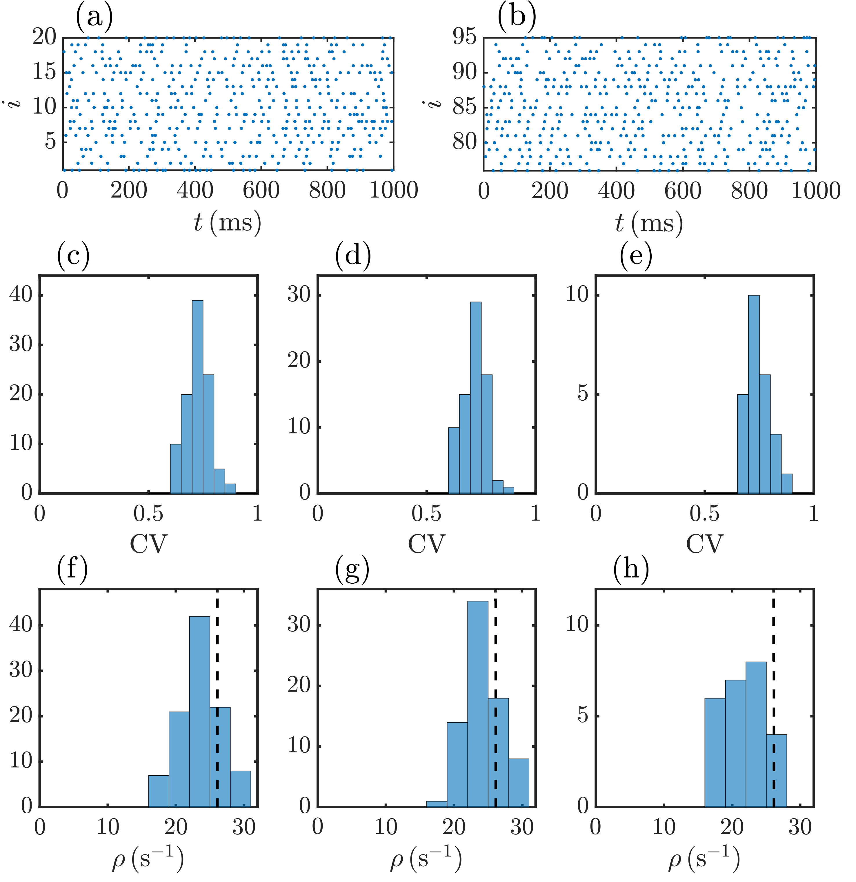 Figure 2
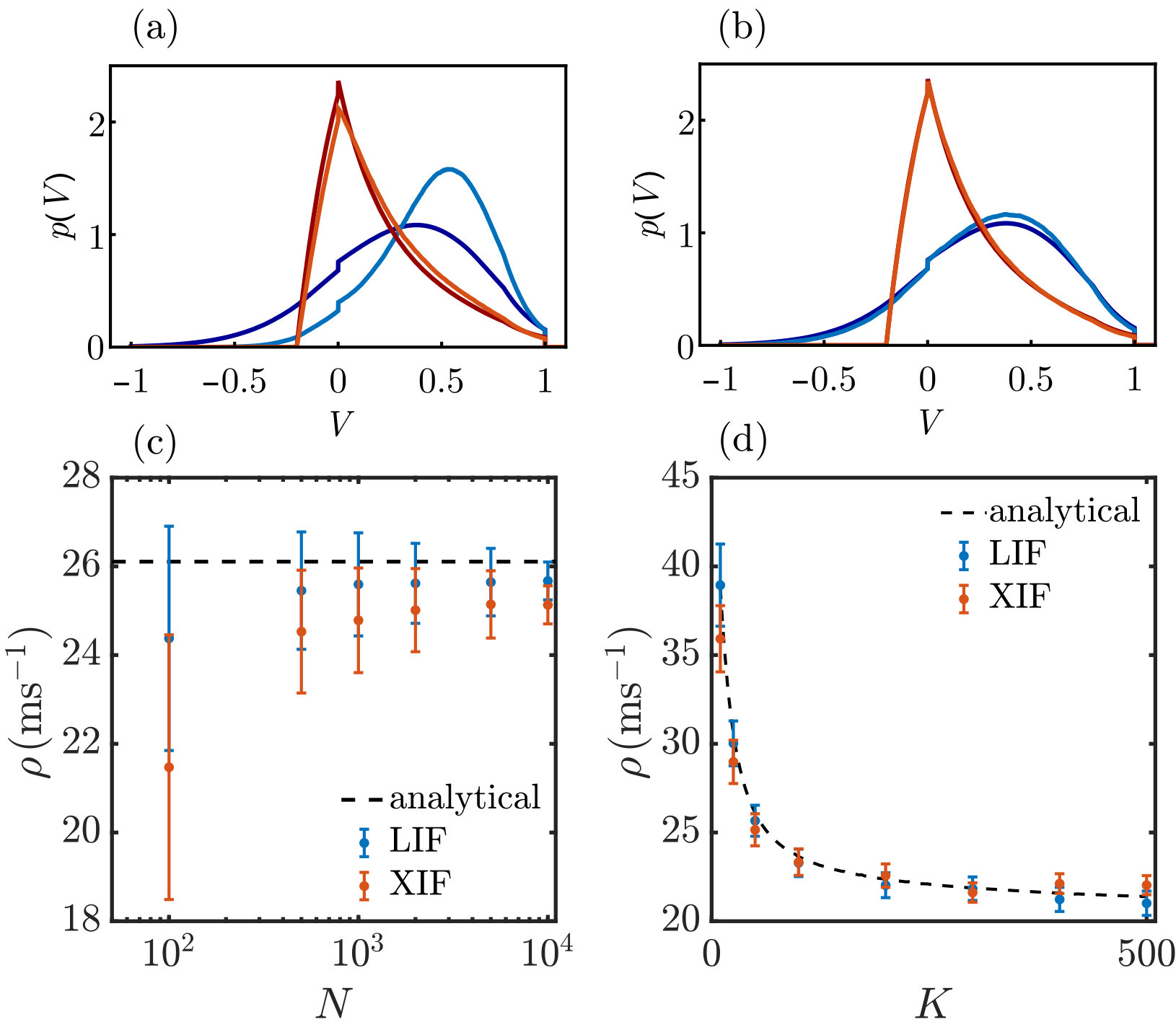 Figure 3
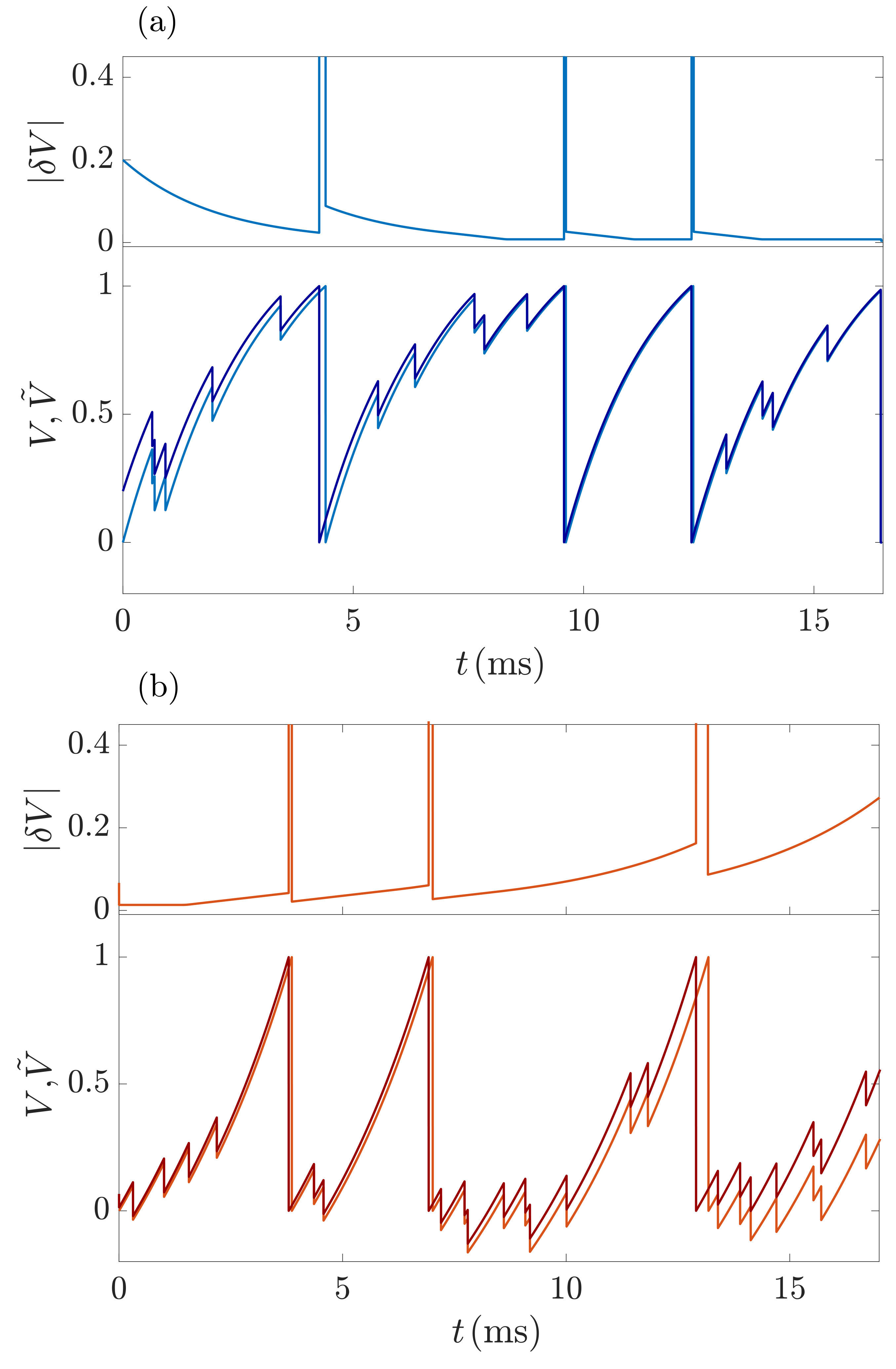 Figure 4
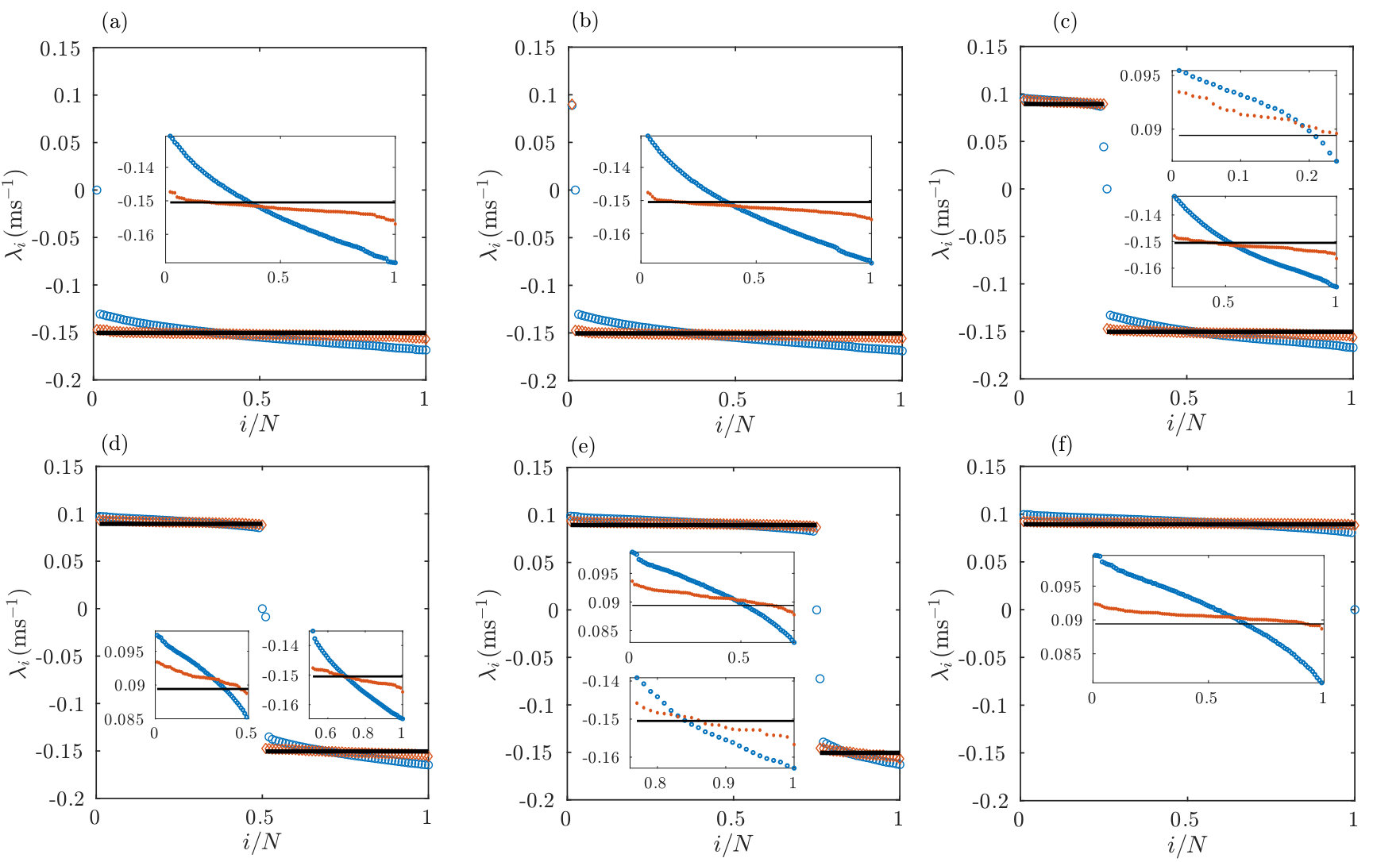 Figure 5
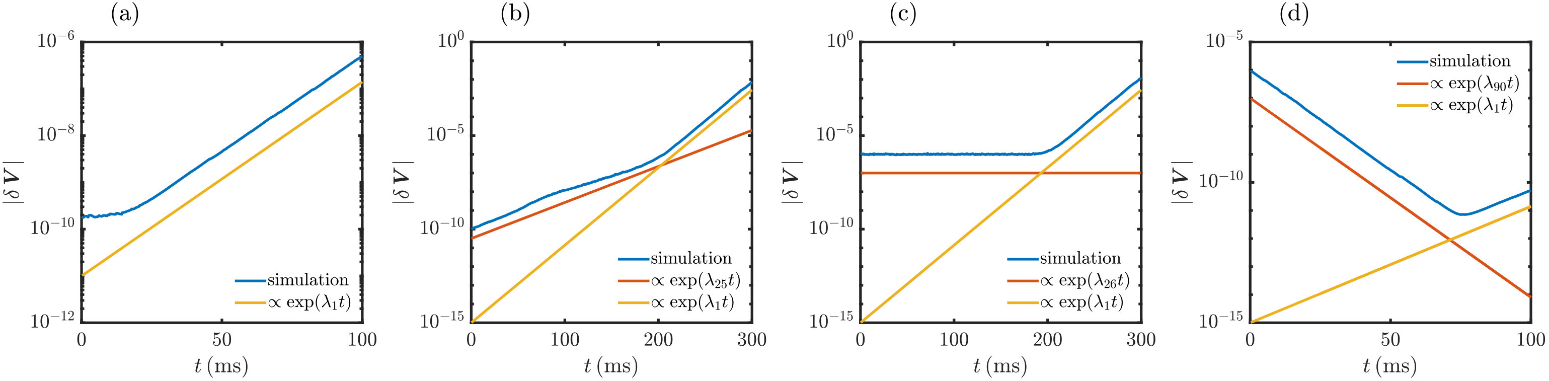 Figure 6
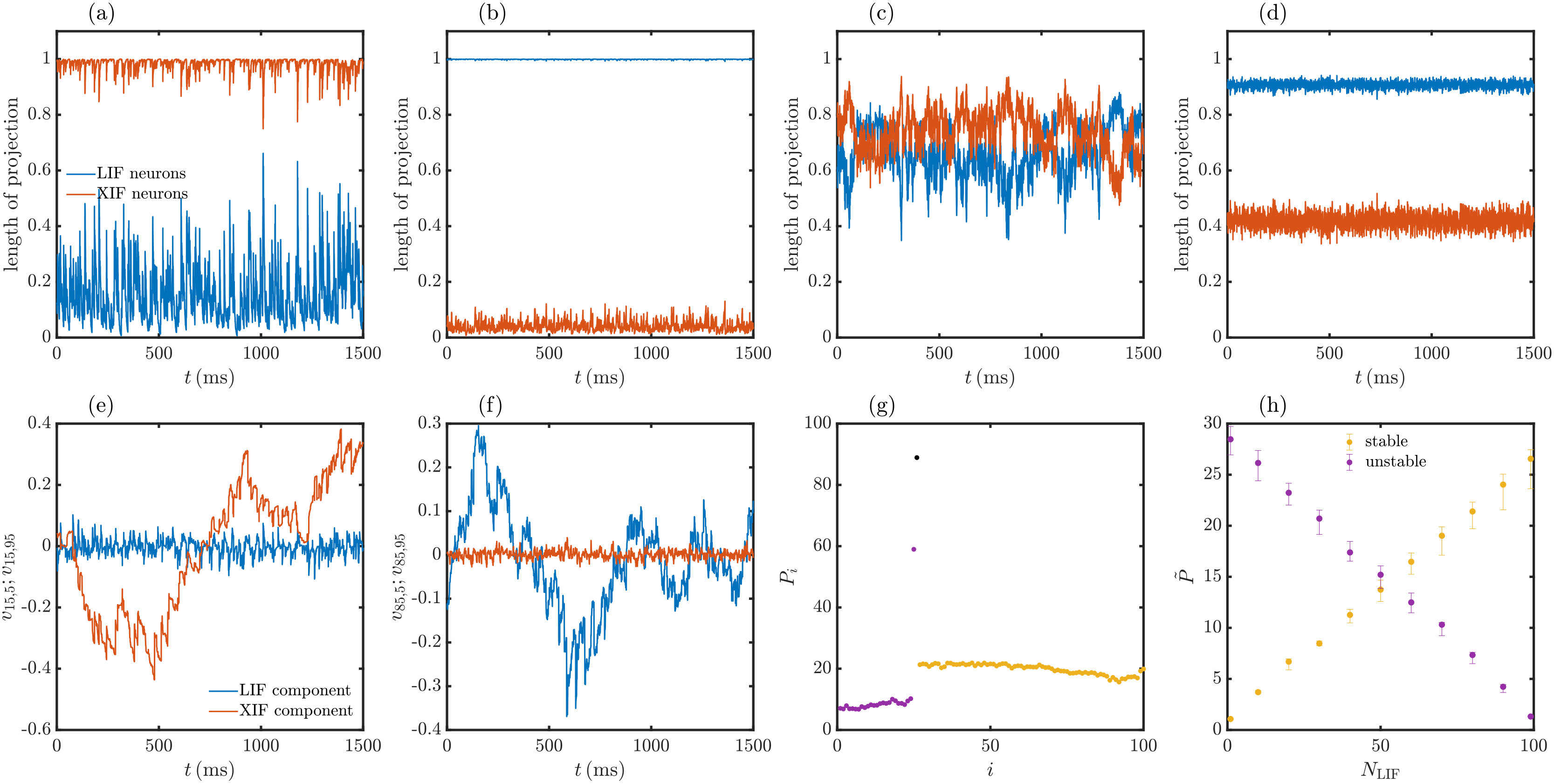 Figure 7
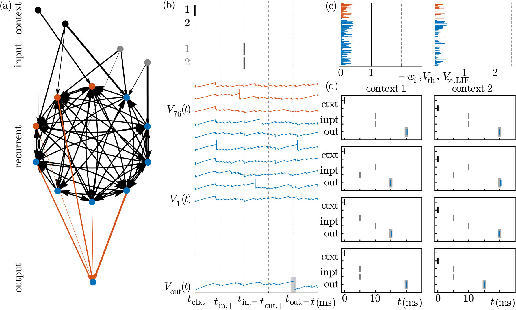 Figure 8
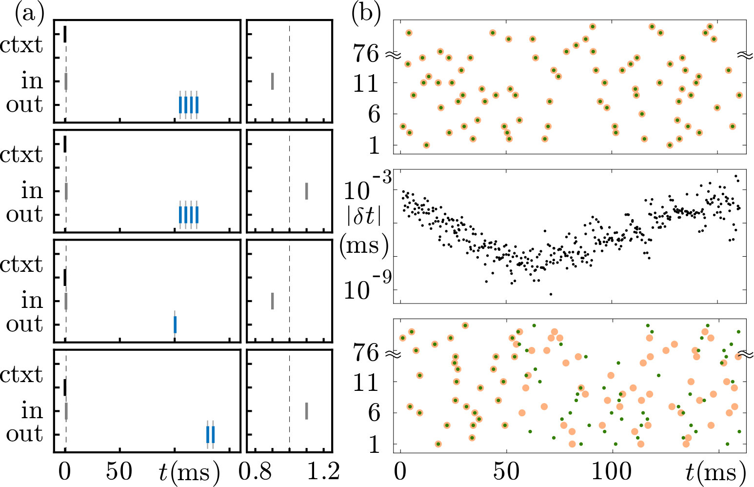 Figure 9
Peer Reviews
No public reviews on file for this paper yet. If you reviewed it on a platform where reviews are public (OpenReview, ICLR, NeurIPS, ICML), you can paste yours below so the community can read it here.
Videos
No videos yet. Explain this paper in a talk, walkthrough, or lecture? Add one.
Dynamics and computation in mixed networks containing neurons that
accelerate towards spiking
Paul Manz
Sven Goedeke
Raoul-Martin Memmesheimer
Neural Network Dynamics and Computation, Institute for Genetics, University of Bonn, 53115 Bonn, Germany.
Abstract
Networks in the brain consist of different types of neurons. Here we investigate the influence of neuron diversity on the dynamics, phase space structure and computational capabilities of spiking neural networks. We find that already a single neuron of a different type can qualitatively change the network dynamics and that mixed networks may combine the computational capabilities of ones with a single neuron type. We study inhibitory networks of concave leaky (LIF) and convex “anti-leaky” (XIF) integrate-and-fire neurons that generalize irregularly spiking non-chaotic LIF neuron networks. Endowed with simple conductance-based synapses for XIF neurons, our networks can generate a balanced state of irregular asynchronous spiking as well. We determine the voltage probability distributions and self-consistent firing rates assuming Poisson input with finite size spike impacts. Further, we compute the full spectrum of Lyapunov exponents (LEs) and the covariant Lyapunov vectors (CLVs) specifying the corresponding perturbation directions. We find that there is approximately one positive LE for each XIF neuron. This indicates in particular that a single XIF neuron renders the network dynamics chaotic. A simple mean-field approach, which can be justified by properties of the CLVs, explains the finding. As an application, we propose a spike-based computing scheme where our networks serve as computational reservoirs and their different stability properties yield different computational capabilities.
I Introduction
Biological neural networks consist of a large variety of interconnected neurons, which communicate via short stereotypical electrical pulses called action potentials or spikes. After a neuron has generated a spike, this travels along the axon and is transmitted to other neurons at synaptic contacts. The electrical membrane potential of the receiving neuron is then changed by an excitatory or inhibitory current pulse. Sufficiently many excitatory inputs in turn lead to spike generation in a receiving neuron. Many biological neural networks generate irregular and asynchronous spiking. This is likely caused by a dynamically balanced network state, in which the average inhibitory and excitatory input current to each neuron sum to a value that is insufficient for frequent spike generation (Gerstein and Mandelbrot, 1964; Shadlen and Newsome, 1994; van Vreeswijk and Sompolinsky, 1996; Denève and Machens, 2016). Spikes are caused by fluctuations in the inputs and the resulting spiking dynamics appear random and irregular.
Irregular dynamics are often chaotic, implying that the dynamics are sensitive to perturbations: initially small ones can strongly grow with time, which results in ultimately large quantitative differences between perturbed and unperturbed trajectories. A powerful tool to quantify this sensitivity and therewith the local phase space structure are the Lyapunov exponents (LEs) and associated with them the covariant Lyapunov vectors (CLVs) (Pikovsky and Politi, 2016; Kuptsov and Parlitz, 2012). The sign of the largest LE indicates whether the system is chaotic and its magnitude equals the long-term average growth or decay rate of generic infinitesimal perturbations. The spectrum of LEs describes the long-term average evolution of volumes spanned by tangent vectors and the change of infinitesimal perturbations in non-generic directions, which are specified by the CLVs. To each LE, there is a CLV. The size of a perturbation in the CLV’s direction changes with an average rate of plus or minus the corresponding LE for long-term forward or backward time evolution, respectively. The CLVs thereby indicate the directions of the unstable and stable manifolds along a trajectory. Furthermore, the spectrum of LEs can be used to derive dynamical quantities such as the Kaplan-Yorke fractal dimension of a chaotic attractor (Frederickson et al., 1983).
In our study, we consider purely inhibitory networks of current-based, oscillating integrate-and-fire type neurons with post-synaptic currents of infinitesimally short duration and instantaneous reset. It has been shown numerically (Zillmer et al., 2006, 2009) and analytically (Jahnke et al., 2008, 2009) that if such networks contain only leaky integrate-and-fire (LIF) neurons, the networks’ irregular balanced state dynamics are stable against infinitesimal and small finite size perturbations and are thus not chaotic but a realization of stable chaos (Politi et al., 1993; Politi and Torcini, 2010). The dynamics ultimately converge to a periodic orbit; the durations of the preceding irregular transients, however, grow exponentially with system size. The stability of the network dynamics is robust against introducing excitatory connections and considering synaptic currents of finite temporal extent (Zillmer et al., 2009; Jahnke et al., 2009) and there is a smooth transition to chaos upon increasing the number of excitatory connections and the duration of synaptic currents. The computational abilities of the stable precise spiking dynamics have not yet been explored, even though the specific structure of the phase space, which is composed of “flux tubes”, may be beneficial and exploitable (Monteforte and Wolf, 2012).
LIF neurons incorporate a leak current as found in biological neurons (Dayan and Abbott, 2001). This increases linearly with increasing membrane potential and leads to dissipation (contraction of phase space volume) in the subthreshold dynamics. When driven by a constant depolarizing input current, the membrane potential therefore has negative second derivative; the neuron has a purely concave so-called rise function. In the considered class of networks, this implies the stability of the microscopic dynamics if only LIF neurons are present (Jahnke et al., 2008, 2009). In biological neurons as well as in neuron models that explicitly model spike generation, such as the quadratic and the exponential integrate-and-fire neuron (Gerstner et al., 2014), the membrane potential accelerates towards a spike for larger membrane potentials. The rise function thus has a convex part. Ref. (Monteforte and Wolf, 2010) showed that networks of quadratic integrate-and-fire neurons that are otherwise similar to those considered in refs. (Zillmer et al., 2009; Jahnke et al., 2008, 2009) exhibit chaos. Furthermore, ref. (Monteforte and Wolf, 2010) computed the spectrum of LEs and quantities that are derivable from them, as well as the statistics of the first CLV, which points into the directions to which a generic perturbation vector aligns in the long term.
Motivated by the above results and by the fact that there are many different types of cortical inhibitory interneurons (Tremblay et al., 2016), in the present study we investigate the impact of inserting a different type of neuron, with non-concave rise function, into inhibitory networks of LIF neurons. To be specific, we insert “anti-leaky” integrate-and-fire (XIF) neurons with purely convex rise function. We choose the letter “X” in the abbreviation to highlight this convexity and the expansion of phase space volume by the flow of the subthreshold dynamics. XIF neurons may be interpreted as a model for a class of biological neurons whose membrane potential lingers in a region where it accelerates towards spiking. Simultaneously, these neurons maintain similar analytical tractability as their leaky counterparts because of their mostly linear subthreshold dynamics. We describe our neuron and network models in detail in the next section. Thereafter, self-consistent firing rates and membrane potential probability distributions for both types of neurons are analytically derived, assuming Poisson input with finite size spike impacts. We then consider the dynamical stability properties and local phase space structures of the network dynamics, computing the entire spectra of LEs both numerically and analytically in a mean-field approximation. We also compute their CLVs to investigate how the stable and unstable directions are related to the different neuron types within the network.
Finally, we consider computations in pure and mixed networks of the considered types and show how the richer phase space structure in mixed ones can be exploited. For this, we propose a reservoir computer based entirely on precisely timed spikes. Reservoir computing has been introduced several times at different levels of elaborateness and in different flavors, in machine learning and in neuroscience (Buonomano and Merzenich, 1995; Dominey, 1995; Jaeger and Haas, 2004; Maass et al., 2002). A reservoir computer consists of a high dimensional, nonlinear dynamical system, the reservoir or liquid, and a comparably simple readout. The reservoir “echoes” the input in a complicated, nonlinear way; it acts like a random filter bank with finite memory as each of its units generates a nonlinearly filtered version of the current input and its recent past while forgetting more remote inputs (Buonomano and Merzenich, 1995; Westover et al., 2002; Maass et al., 2002; Jaeger and Haas, 2004). The simple, often linear readout can then be trained to extract the desired results, while the reservoir is static. In our scheme, the output neuron is spiking and thus nonlinear, the desired outputs are trains of precisely timed spikes. The learning thus requires different approaches than learning of conventional continuous targets; gradient-descent based methods (LeCun et al., 2015) fail due to the discontinuity at the threshold as well as methods that require errors to be small but finite (Sussillo and Abbott, 2009). A number of algorithms have been suggested to learn precisely timed spikes (Ponulak and Kasiński, 2010; Florian, 2012; Mohemmed et al., 2012; Xu et al., 2013; Memmesheimer et al., 2014; Albers et al., 2016; Zenke and Ganguli, 2018; Huh and Sejnowski, 2018), mostly using heuristic approaches. For our readout neuron, we can use the Finite Precision Learning scheme (Memmesheimer et al., 2014). It has been shown to generically converge if the input-output relation is realizable at all, which explains its numerically found superior learning abilities (Albers et al., 2016).
II Mixed networks of neurons with concave and convex rise function
We consider a recurrent network with neurons. The th spike of neuron , which is sent at time , generates a postsynaptic current pulse in neuron . Here is the weight of the inhibitory connection and is a possible voltage-dependent modulation, which depends on the membrane potential of neuron just before input arrival, given by the left-hand side limit . We assume that all excitatory inputs to neuron can be gathered into a constant excitatory external input current and that the remaining explicitly modeled recurrent inhibition is fast (Jahnke et al., 2008; Monteforte and Wolf, 2012; Olmi et al., 2017). We further assume that there is a leak term with prefactor . Taken together, we model the subthreshold membrane potential dynamics of neuron by
[TABLE]
When reaches the spike threshold at time , , it is reset, , and a spike is emitted. This, in turn, generates in a postsynaptic neuron a current pulse as introduced above, which causes to decrease in jump-like manner from to . The rise function, i.e., the membrane potential dynamics with in absence of recurrent inhibitory input (Mirollo and Strogatz, 1990; Memmesheimer and Timme, 2006), reads
[TABLE]
It is concave for and convex for .
There are two types of neurons in our networks: LIF neurons with dissipation and concave rise function, which obey Eq. (1) with , and anti-leaky XIF neurons with convex rise function, which obey Eq. (1) with , see Fig. 1. The membrane potential dynamics of an LIF neuron has a globally attracting fixed point at , if there is no threshold for spike generation and no inhibitory input. We assume , so neurons without inhibitory input periodically spike and reset. For our study it is sufficient to endow the LIF neurons with a simple, current-based synapse model, setting . A coarse approximation of the membrane potential dynamics without threshold and neglecting input fluctuations yields , where is the average inhibitory input current. In the balanced state, its attractor at is below or close to the spike threshold, such that spikes are always or typically generated by input fluctuations, more specifically by periods of less than average inhibition.
In the absence of inhibitory input XIF neurons have an unstable, repelling fixed point at . If the membrane potential starts above this separatrix, it increases exponentially towards the threshold. When it reaches there, the neuron spikes, its membrane potential resets to zero, increases towards the threshold again and so forth: XIF neurons oscillate and spike periodically for any , if there is no inhibitory input. If the membrane potential starts below the separatrix, it decreases exponentially to . Also in the presence of recurrent inhibitory inputs an XIF neuron is unrecoverably switched off once its membrane potential falls below , since the inputs only decrease the membrane potential further. Averaging over the inhibitory inputs as before yields an effective separatrix at . Membrane potentials falling below it have a tendency to further decrease, causing the neuron to effectively switch off. This can be also seen from the phase response curve of XIF neurons, which gets steeper for negative phases, in contrast to that of LIF neurons which becomes flatter, see Fig. 1c. In other words, in XIF neurons an incoming inhibitory input at a low potential still above the separatrix (and thus at a low phase) has a larger effect in the sense that it delays the next spiking more than the same input arriving at a higher potential. As a consequence, we observe in networks containing XIF neurons with purely current-based input [] that many of these neurons are first effectively and then unrecoverably switched off, if the network dynamics are irregular and the inhibitory inputs are therefore strongly fluctuating. In order to prevent this biologically implausible phenomenon, we introduce a voltage dependence
[TABLE]
of the input coupling strength, where is the Heaviside theta function. Inhibitory inputs arriving at a membrane potential lower than then do not induce a further decrease. This provides a simple conductance-based model for the synapses, where the driving force of the current vanishes below and is constant above. We assume for all to exclude unrecoverable switching off and . We exemplarily checked that the overall network dynamics and their stability properties remain qualitatively unchanged, if we also endow the LIF neurons with these synapses.
For simplicity, we choose the parameters of all LIF and of all XIF neurons identical, i.e., , etc., if neuron is an LIF neuron, and , etc., if neuron is an XIF neuron. The spike threshold and reset potentials are and , independent of the neuron type. We set to avoid any effective switching off of XIF neurons. Coupling strengths are homogeneous, if the coupling is present. To keep the number of relevant parameters small, we further choose . The additional choice leads already in absence of recurrent inhibition to a higher spike rate in XIF neurons, since
[TABLE]
whereas in LIF neurons,
[TABLE]
As a consequence, we observe that in a mixed network the XIF suppress the LIF neurons, which become quiescent. Using the analytical results of the next section, we therefore rescale such that the spike rates in both populations are identical. Further, we fix the neurons’ indegree to the same number , implying that is identical for each neuron . This reduces quenched noise (van Vreeswijk and Sompolinsky, 1998) and avoids strong differences in average spike rates and switched off neurons.
With the described network model setup, we observe balanced states of asynchronous irregular spiking activity for any ratio of neurons with concave and convex rise function, see Fig. 2 for an illustration.
III Network firing rate and membrane potential distributions
Mean-field theories have been developed in statistical physics (Kadanoff, 2009) and are frequently used in computational neuroscience, see, for example, refs. (van Vreeswijk and Sompolinsky, 1998; Brunel, 2000; Breuer et al., 2014; Schuecker et al., 2018). The basic idea is to average the interactions in a high-dimensional system to obtain for each element an effective action, which is not influenced by this element anymore. One can thereby reduce a high-dimensional problem to low-dimensional ones. In this section we analytically determine the steady-state firing rate and the voltage probability densities for LIF and XIF neurons in mixed networks using a mean-field approximation. We use the results to obtain neuron parameters that lead to the same average firing rates for both neuron types and thus to homogeneous firing rates in the entire network. In addition we employ the firing rates to analytically approximate the Lyapunov spectrum of the network dynamics using a mean-field approach in Sec. IV.1.
We approximate the superposed input spike trains to a neuron by a Poisson spike train with a given rate, i.e. we assume that all input spikes are sent independently of each other. A common approach is to additionally consider the limit of a large number of small inputs. The neuron dynamics can then be approximated by a diffusion process, which allows to compute firing rates and membrane potential distributions (Tuckwell, 1988; Burkitt, 2006). This diffusion approximation assumes that the inputs have (infinitesimally) small amplitude and arrive at (infinitely) high rate. Here we use a shot noise approach, which accounts for the finite input rate and size of individual inputs (Tuckwell, 1988; Burkitt, 2006), in the recent formulation of refs. (Richardson and Swarbrick, 2010; Olmi et al., 2017). This allows to more accurately obtain the firing rates and membrane potential distributions. In particular, the fact that in our networks the voltage probability density does not go to zero at threshold is reflected. We shortly review the approach for LIF neurons (Richardson and Swarbrick, 2010; Olmi et al., 2017; Angulo-Garcia et al., 2017) and then extend it to XIF neurons with the voltage-dependent coupling Eq. (3).
The shot-noise approach (like the diffusion approximation) is based on the continuity equation for the voltage probability density . For our neuron models it reads
[TABLE]
where is the drift probability current with velocity . and are source terms incorporating the effects of inputs and resets of the neuron’s membrane potential .
For the LIF neuron without the voltage-dependent input, inhibitory input spikes arriving when the considered neuron is at a voltage give rise to a sink at , whereas spikes arriving when the neuron is at a voltage give rise to a source at . We therefore have a first source term
[TABLE]
with the rate of input spikes. We note that refs. (Richardson and Swarbrick, 2010; Olmi et al., 2017; Angulo-Garcia et al., 2017) include this term in the probability current. The second source term is due to the spike and reset mechanism of the neuron model. Its threshold and reset act as Dirac delta sink and source at the corresponding discrete voltages,
[TABLE]
This term is proportional to the instantaneous firing rate of the stochastic neuron dynamics or, in other words, to the probability current through the threshold [].
We investigate stationary network dynamics, which are described by constant and and time-independent . For these Eq. (6) reduces to the linear delay differential equation (or differential-difference equation)
[TABLE]
Dividing Eq. (9) by yields an equation for the rescaled density , which is independent of the unknown steady-state firing rate . This equation can be integrated for example with the method of steps (Hale and Verduyn Lunel, 1993). The integration starts with the “initial conditions” for and thus slightly below . The normalization of allows us to compute via
[TABLE]
To obtain an analytic expression for , one applies a bilateral Laplace transform . We can focus on ; yields . The Laplace transform of the rescaled Eq. (9) results in a linear first-order ordinary differential equation for ,
[TABLE]
It can be solved by variation of constants. The solution of the homogeneous equation is
[TABLE]
with an arbitrary constant and
[TABLE]
Here, is the exponential integral and is the Euler-Mascheroni constant. The solution of the full equation then reads
[TABLE]
Since the support of is bounded from above by , . To balance the faster exponential growth of its prefactor , the bracket on the right hand side of Eq. (14) needs to vanish for large . We thus have
[TABLE]
For an XIF neuron without voltage-dependent synapses there is no stationary membrane potential probability density This is because for any time there is a finite probability that the membrane potential of a neuron jumps below and thereafter tends to minus infinity. In contrast, for an XIF neuron with the voltage dependence Eq. (3), exists and we may use the same approach as for the LIF neuron to determine it together with the firing rate. Since membrane potentials do not drop below , we focus on the interval , where can be nonzero. The couplings’ voltage dependence enters the source term in Eq. (6): If is below , incoming spikes have no effect and the sink term due to them vanishes. Eq. (7) therefore changes to
[TABLE]
where we used that in the relevant voltage range such that a modification of the source term is unnecessary. The stationary continuity equation becomes
[TABLE]
which can be rescaled and integrated using the method of steps to obtain , and as before. The nonlinear prefactor however, impedes the derivation of via Laplace transform.
We apply the above results to find mixed networks in which LIF and XIF neurons have similar firing rates. Eq. (15) provides a map from the input to the output rate, . Eq. (17) implicitly defines such a map for XIF neurons. The firing rate of the LIF and XIF neurons in the desired mixed network needs to solve both self-consistency equations
[TABLE]
with the neurons’ indegree . We employ Eq. (19) to compute for XIF neurons. Thereafter, we adapt the parameters of Eq. (18) such that the same becomes a solution. Specifically, we solve for , keeping the other parameters fixed.
Fig. 3 compares the voltage densities and rates obtained from the shot noise approach with those of an LIF and an XIF neuron that receive input spike trains as they are generated in the recurrent network of Fig. 2. There is a pronounced discrepancy between the densities and rates for an LIF neuron for and small , because both the individual (see Fig. 2a-e) and the superposed input spike trains in these dense networks are more regular than Poisson spike trains. Removing spatial correlations for example by increasing reduces the discrepancy, see Fig. 3b-d and App. VII.1 for further analysis. Such input spike trains reduce the variance of the voltage and generate a that is more concentrated around the value , where is the average inhibitory input current as discussed in Sec. II. For the XIF neuron, the input spike train statistics has less impact on . Presumably, this is because voltage excursions due to input fluctuations are anyways suppressed by the voltage dependence of the input strength (for potentials near ) and by the drive towards threshold (for larger potentials). We note that the assumption of Poisson input spike trains is the only approximation in the chosen approach, such that sampled membrane potential distributions of neurons with Poisson input match the analytical ones up to the sampling noise as shown in App. VII.1.
IV Growth of dynamical perturbations
IV.1 Mean-field approach
After obtaining the spike rates and membrane potential distributions using a statistical mean-field theory, we investigate the mixed network dynamics from a dynamical systems perspective. We first analytically determine the Lyapunov spectrum using again a mean-field approach. It focuses on the evolution of perturbations to a single neuron and treats the input from other neurons as external. Specifically, we disregard perturbations of the rest of the network including those generated by the considered neuron’s changed spiking. Inputs thus arrive at the same times in the perturbed and in the unperturbed system and do not change the neuron’s perturbation. Fig. 4 illustrates this and compares the resulting evolution of a perturbation of an XIF neuron and of an LIF neuron: The perturbation of the XIF neuron gradually increases as long as it is not spiking, while that of the LIF neuron decreases. Conversely, in the XIF neuron spiking and resetting reduces perturbations, while it increases them in the LIF neuron; compare the values of the (finite size) distance between two neighboring trajectories and in Fig. 4a,b before and after a spike event has taken place in both the perturbed and the unperturbed dynamics. To assess the influence of these two processes, we first note that in a freely oscillating neuron they need to cancel each other such that perturbations persist on average and the LE is zero. We then note that the inhibitory inputs do not affect perturbations but prolong the subthreshold evolution between spikes. Its impact therefore dominates, and perturbations in XIF neurons grow over time, while they shrink in LIF neurons. This does not depend on the specifics of the LIF and XIF dynamics but is a consequence of the curvature of the rise function and the inhibitory inputs.
In App. VII.2, we make the gained intuitive understanding precise by quantifying the growth of perturbations and the resulting LE. For this, we describe the dynamics by a sequence of discrete maps from the state at a time (infinitesimally) shortly after generation of a spike to the state at a time shortly after generation of the next spike. The discrete time dynamics of small perturbations are then given by the “single spike Jacobians” (Monteforte and Wolf, 2010, 2012) . For the effective single neuron dynamics here, they reduce to scalar factors
[TABLE]
with the free firing rate (Eq. (4) or (5)) of the neuron.
The growth rate of perturbations and thus the mean-field LE are given by the long-term average of Eq. (20),
[TABLE]
This expression confirms the intuitive understanding that without perturbed inputs the growth rate depends (i) on the growth rate during subthreshold evolution and (ii) on the prevalence of subthreshold evolution () or spike sending () relative to the free neuron case. In particular, without input we have and if the neuron is silenced . In our inhibitory networks we have such that for XIF and for LIF neurons. In networks in the balanced state, the actual spike rate is much smaller than the spike rate of a neuron if only excitation is present. Since in our networks the latter equals the spike rate of the freely oscillating neuron, we have . Thus the mean-field approach indicates that the growth rate of perturbations is mainly given by the subthreshold growth. The mean-field approach further indicates that a single XIF neuron renders the entire network dynamics unstable and that the number of unstable directions equals the number of XIF neurons in the network, while the number of stable directions equals the number of LIF neurons. This, however, does not give rise to a zero LE, which occurs in the full autonomous network due to time-translation symmetry. The mean-field spectrum and the rule for the number of stable and unstable directions can thus only be an approximation to the exact results.
Eq. (21) together with the analytical results Eqs. (18),(19) for give a fully analytical estimate of the Lyapunov spectrum. Since all LIF or XIF neurons have the same analytical rate estimates and leak strengths, the spectrum consists of identical negative and identical positive exponents, see Fig. 5. Due to quenched noise from random coupling, the rates in the actual network are distributed. We can account for this by inserting the numerically measured rates into Eq. (21), see Fig. 5.
IV.2 Network single spike Jacobian
To derive exact Lyapunov spectra we need to take into account the spreading of perturbations in the network. For this, we compute the full single spike Jacobian , which is a map from tangent vectors at the point in phase space to tangent vectors at , where is the state of the system at time . The resulting components of read
[TABLE]
for an LIF or an XIF neuron , where is the index of the neuron sending the th spike, see App. VII.3 for details. We note that the mean-field theory accounts for the diagonal terms of this Jacobian.
IV.3 Volume contraction
Owing to the simple form of the single spike Jacobians we can find an analytical expression for the full network dynamics’ expansion rate of infinitesimal phase space volumes or, equivalently, for the sum of the LEs. The result in terms of the neuronal spike rates in the network is exact. It allows to analytically compute the Lyapunov spectra for two neuron systems and offers a test for the accuracy of their numerical estimates in larger networks.
The volume expansion and the sum of LEs are given by the time averaged logarithms of the determinants of the Jacobians (Pikovsky and Politi, 2016). We thus have
[TABLE]
in terms of single spike Jacobians (Monteforte and Wolf, 2012). In App. VII.4 we exploit the specific form of to compute with the matrix determinant lemma. The subsequent time averaging yields
[TABLE]
Notably, this shows that our mean-field theory yields an exact expression for the volume contraction rate and the sum of LEs: the estimate with Eq. (21) agrees with the exact expression Eq. (24).
IV.4 Numerical computation of the Lyapunov spectrum
The single spike Jacobians (22) allow us to iteratively compute the largest LE and the full Lyapunov spectrum (Monteforte and Wolf, 2010; Pikovsky and Politi, 2016; Engelken, 2017), see also App. VII.6. In short, for the largest LE, one iterates an initial random perturbation vector by the single spike Jacobians, stores its growth every few steps and thereafter renormalizes it to its initial magnitude. The long-term average of the growth rate equals . For the full spectrum, one iterates a system of orthogonal perturbation vectors with the single spike Jacobians. Every few steps, one records the growth of the different vectors. Thereafter one reorthogonalizes, always in the same order, and finally renormalizes the vectors. The long-term average growth rate of the first vector then equals , that of the second equals etc. Ref. (Engelken, 2017) suggested an efficient method to compute the Lyapunov spectrum and applied it to large networks; we use some of the ideas in our implementation.
For networks consisting only of LIF neurons we find in agreement with previous work (Zillmer et al., 2006; Jahnke et al., 2008, 2009; Zillmer et al., 2009) and our mean-field theory that the largest nontrivial LE is negative, see Fig. 5a. However, we also find that already the presence of a single XIF neuron renders the largest LE positive, see Fig. 5b, indicating chaos in agreement with the mean-field theory. The computations also confirm that the destabilization of a network by a single XIF neuron is a special case of a general rule, namely that each XIF neuron introduces about one positive LE. This holds independently of and , see Fig. 5 and App. VII.5. The trivial (zero) exponent is an exception to the rule. Our numerical results indicate that it replaces a negative exponent if there are more LIF than XIF neurons in the network and a positive exponent otherwise. There is also good quantitative agreement with the mean-field spectrum, in particular the exponents are close to and However, also when inserting the measured spike rates into Eq. (21) some discrepancy remains, showing that the spread of perturbations in the network and their transfer between neurons has a pronounced effect on their growth.
V Stable and unstable directions
V.1 Lyapunov vectors and perturbation growth
To further elucidate the local phase space structure, we numerically investigate the characteristics of the perturbations that grow according to the individual LEs, i.e. how they are distributed across neurons and how they change during evolution. This will, in particular, allow us to understand why the mean-field theory works well. The directions of the perturbations are given by the CLVs or, in other words, by the stable and unstable manifolds along the trajectory (Kuptsov and Parlitz, 2012; Pikovsky and Politi, 2016).
The th CLV at a point in phase space is a normalized tangent vector that grows with long-term average rates and when evolved forward and backward in time. We call it a stable CLV if and an unstable one if . We assume for simplicity that all LEs are different; the vector is then unique up to its orientation. Consider a trajectory that reaches shortly after the spike time the state . Using the single spike Jacobians , may be defined as the tangent vector satisfying
[TABLE]
where and are chosen sufficiently large. The definition can be straightforwardly extended to states between spiking events. Both of its parts are important: The first part alone does not uniquely define the direction of , since adding any vector with growth rate less than yields the same asymptotics. The second part excludes such an addition, since its shrinkage rate is slower than and thus yields a different dominant asymptotics of backward evolution. As anticipated by the notation, the vector depends only on the state but not on the time when reaches it. Furthermore, the definition ensures covariance, that is the evolution of infinitesimal perturbations (the tangent flow) maps CLVs to CLVs. At subsequent spike times we thus have
[TABLE]
The extension to states between spike times is again straightforward: the covariance implies that we can obtain CLVs at a state between spike times and by propagating forward with the Jacobian of subthreshold evolution.
We compute the CLVs in a dynamical manner by forward and restricted backward propagating sets of vectors, following refs. (Ginelli et al., 2007; Pikovsky and Politi, 2016). Appendix VII.6 provides a short description of the method. We note that the dynamics of our system are not invertible: given a state there is no unique way of propagating it back in time. This is because an ambiguity can arise at states where one neuron is at the reset potential; we generally cannot tell whether it was reset or crossed the reset potential from below (unless some postsynaptic neuron is too near to threshold to be able to have just received a spike). It is, however, still possible to compute the Lyapunov vectors by backward propagating along the trajectory that was previously taken for the forward propagation (Ginelli et al., 2007).
V.2 Stable and unstable directions in mixed networks
The CLVs yield the directions in which small but finite perturbations evolve according to the different LEs as shown in Fig. 6. We find that they generally contain perturbations to a variety of neurons and that they strongly change their direction during evolution. More specifically, we observe that the stable and unstable CLVs stay approximately confined to the subspaces of (strictly speaking: perturbations to) LIF and XIF neurons, respectively. Fig. 7a-d illustrates this by displaying the lengths and of the projections of different CLVs onto the subspaces of LIF and XIF neurons. Here and in the following we assume that the LIF and XIF neurons have the indices and , respectively. Fig. 7e,f further illustrates the confinement and shows the large temporal variability of single CLV components that are not close to zero. The confinement does not hold exactly since perturbations of LIF neurons usually also give rise to perturbations of XIF neurons and vice versa. In networks with inhomogeneous spike rates, we observe that single neurons that are strongly suppressed by inhibition have CLVs more aligned to them, because their perturbation spreads less in the network due to their lack of spiking.
We further quantify the localization of the CLVs using an inverse participation ratio (number) (Kramer and MacKinnon, 1993; Ginelli et al., 2007), which we define for the th CLV as
[TABLE]
Here, is an average over sufficiently many events and we use that the CLVs are normalized, . The participation ratio measures how many components contribute to a vector. If, for example, the vector always has only one nonzero component, . If there are always nonzero components of equal size, . We observe that the participation ratio of unstable CLVs increases approximately linearly with the number of XIF neurons starting with at , consistent with a delocalization of these CLVs between the present XIF neurons, see Fig. 7g,h. for stable CLVs increases likewise with the number of LIF neurons. The trivial CLV has a participation ratio close to , because the components of the tangential vector and thus the components of the CLV have roughly similar size.
Our mean-field approach uses the assumption that each LE is independently generated by the growth or shrinkage of a single neuron perturbation, with negligible influence of the perturbation’s spread and backreaction in the network. Its suitability can now be understood as follows: The approximately stable CLVs are confined to the -dimensional subspace of perturbations to LIF neurons. The stable CLVs thus form a basis of the subspace of perturbations to LIF neurons. Likewise the unstable CLVs form a basis of the subspace of perturbations to XIF neurons. At each time point, a perturbation to a single LIF neuron can therefore be expressed as a linear combination of stable CLVs, while a perturbation to an XIF neuron can be expressed as a linear combination of unstable CLVs. The stable CLVs have similar decay rates (negative LEs) and the unstable CLVs have similar growth rates (positive LEs), see Fig. 5. Any linear combination of only stable or only unstable CLVs inherits this decay or growth rate. This holds in particular for the perturbation of a single neuron. At each time point the perturbation to a single LIF or XIF neuron thus grows according to the negative or according to the positive LEs, respectively. The mean-field approach therefore yields good results.
VI Computations with precisely timed spikes
VI.1 Network architecture and task design
In the following, we employ our networks for computations. In particular, we investigate how their different phase space structures and CLVs may be exploited in specific tasks. This requires a computational scheme based on precise spiking, which is affected by the phase space structure. We design a setup where one of our recurrent neural networks acts as a kind of computational reservoir (Maass et al., 2002; Jaeger and Haas, 2004; Monteforte and Wolf, 2012), in the sense that it randomly nonlinearly filters its inputs. An output neuron receives the generated spikes and learns to generate desired outputs, see Fig. 8a.
Inspired by experimental and computational neuroscience paradigms (Maren et al., 2013; Mante et al., 2013), we assume that the networks receive inputs from context neurons, whose spiking defines the computation to be executed in the specific trial, and from input neurons. Their synaptic weights as well as the recurrent ones are static; only the output weights are learned. At the beginning of each trial, all membrane potentials are reset to zero. The recurrent network dynamics are therefore identical in trials with the same context and input neuron spikes. To keep the computational scheme consistent, we specify trains of precisely timed spikes as desired outputs.
The output neuron is an LIF neuron as used in the recurrent network. The subthreshold dynamics of its membrane potential are thus given by
[TABLE]
where are the output weights, is the threshold, the output spikes, the asymptotic potential and the number of spiking neurons in the recurrent network. Initially , and the are are drawn randomly from the uniform distribution over . We use Finite Precision Learning (Memmesheimer et al., 2014) to learn the input-output tasks. The shapes of the post-synaptic potentials in our single neuron dynamics are different from those in ref. (Memmesheimer et al., 2014) and there is an additional constant driving term. The learning rule can be readily adapted to this: We consider and cast it into the form . Spikes are generated when reaches zero. At each time , we thus have a kind of perceptron classification task, where , and are the “weights” to be learned. The “inputs” belonging to these weights are
[TABLE]
Following ref. (Memmesheimer et al., 2014), we assume a tolerance window of size around each desired spike (we use 1\text{,}\mathrm{ms}$$ throughout). There are now two kinds of errors: (i) undesired spikes, i.e. spikes out of a tolerance window or second spikes within a tolerance window (, the error time is the spike time) and (ii) missing spikes within a tolerance window (, is the end of the tolerance window). The dynamics are stopped at the first error and , and are corrected according to the perceptron rule,
[TABLE]
with learning rate (we use ). To focus on networks with inhibitory neurons throughout the article, we restrict the output weights to be inhibitory by clamping them at zero when they would become excitatory during learning. We note that a missed spike generates increases in and as well as a decrease in to foster spiking. If an undesired spike occurs, the signs are reversed.
VI.2 Switchable temporal XOR/AND
We exemplarily consider two tasks. In the first, the network of Fig. 8a learns to execute in context 1 a temporal XOR and in context 2 a temporal AND computation, see Fig. 8b-d. The weights from context and input neurons to the recurrent network are drawn randomly from the uniform distribution over . At the beginning of a trial, at 0\text{,}\mathrm{ms}, context neuron 1 or 2 sends a spike, specifying the context. Thereafter each input neuron sends a spike, either at time $t_{\text{in,+}}=$5\text{\,}\mathrm{ms} (“”-input) or at 10\text{,}\mathrm{ms} (“$-$”-input). The desired output spike is at $t_{\text{out,+}}=$15\text{\,}\mathrm{ms} (“”-output) or at 20\text{,}\mathrm{ms}$$ (“”-output), depending on the context and the input spike times.
The considered networks learn the task easily, whether the reservoir consists of LIF or XIF neurons or of a mixture of both. The example with a mixed network displayed in Fig. 8 (same network as in Figs. 2, 5c, 6 and 7) required 53 learning cycles, where in each cycle the four input-desired output patterns of both contexts were presented. The networks cannot learn the task, if the recurrent network dynamics at the desired output times are too similar for different contexts and input conditions. This happens for recurrent LIF networks, if the context or input neurons have coupling strengths that are so weak that the perturbations due to different input timing are small. The states are then within the same flux tube and the perturbation decays up to a time shift. In XIF and mixed networks, the recurrent dynamics are too similar if there is insufficient time for the perturbation to grow and spread before the first desired output.
VI.3 Detect or ignore input time differences
In the second task, the system has to ignore a difference in input timing in context 1 and to detect it in context 2. The network setup is as in Fig. 8a, except that there is only one input neuron. This sends a spike at or at (1\text{,}\mathrm{ms} 0.1\text{,}\mathrm{ms}). The output neuron shall generate in context 1 for both input conditions the same output, a burst of four spikes at $t=$105\text{\,}\mathrm{ms}$,$110\text{\,}\mathrm{ms}$,$115\text{\,}\mathrm{ms}$,$120\text{\,}\mathrm{ms}. In context 2 it shall detect the difference and highlight it by sending one spike at 100\text{,}\mathrm{ms} (input at $t_{\text{in},+}$) or two spikes at $t=$130\text{\,}\mathrm{ms}$,$135\text{\,}\mathrm{ms} (input at ). For this task, for simplicity we assume that the impacts of input neurons do not depend on the membrane potential, i.e. for them . Further, we allow context and input weights to be excitatory and inhibitory.
We find that networks with the previously chosen random parameters of external weights drawn from usually cannot solve the task (criterion: no convergence within 50000 cycles). The reason is different for pure LIF reservoirs and for reservoirs containing XIF neurons: In a pure LIF reservoir, the small difference in input times leads to state perturbations that are usually in the same flux tube. These decay to a temporal shift until the time of the desired outputs. The readout neuron thus cannot learn to generate two different output patterns as required in context 2. In presence of XIF neurons, the dynamics are locally unstable. The small input difference is amplified in both contexts and the reservoir spiking is different for all four patterns at the times of the desired output. The network therefore has to learn four input-output relations with eleven output spikes and silence periods in between, without being able to take advantage of the fact that two of the four output patterns are identical. This typically exceeds its learning capacity. We also observe for our parameters that the dynamics of the pure LIF reservoir can leave its flux tube due to the perturbation. If this happens only for context 2, the system can often learn the task.
To solve the problem, we design the network such that, reliably, in context 1 but not in context 2 the input differences leave the reservoir spiking at the time of the desired outputs largely unaffected. This can be achieved by choosing the context and input couplings such that the input difference generates a state perturbation along a stable CLV of the reservoir dynamics in context 1. In contrast, for context 2 the state perturbation should have a component in the direction of an unstable CLV such that it is quickly amplified. The setup requires mixed networks with both types of CLVs. We note that an alternative approach might exploit the dichotomy of large and small perturbations, which do and do not leave the flux tubes of pure LIF networks.
To derive appropriate weights, we compute the state perturbations in the reservoir assuming that in the “unperturbed” system the input arrives at . We there have
[TABLE]
where is the coupling strength from the input neuron to neuron . In the “perturbed” system, the input arrives shifted by (here: ), such that we have in linear approximation
[TABLE]
To compute a perturbation in the that corresponds to the perturbation due to the temporal shift of input, we propagate the perturbed potential in linear approximation from to ,
[TABLE]
A temporal input difference that should be ignored should be proportional to a stable CLV at the state , i.e.
[TABLE]
We choose the same recurrent network as in Figs. 2, 5c, 6 and 7 and the same CLV as in Fig. 6d at 0\text{,}\mathrm{ms}$$, i.e. and
[TABLE]
where is the state at which the vector was recorded. Context input 1 determines the state at by fixing the initial conditions of the dynamics. We choose as context input weights
[TABLE]
which lead to Eq. (40) after free propagation until and receiving of the input . To ensure that the perturbation in context 2 has a component in the direction of an unstable CLV, it suffices to choose a random context weight vector, such that and is typically not a stable CLV or a linear combination of stable CLVs at the state . We randomly permute the entries of to obtain .
We find that the network constructed in this way can reliably learn the task. The example displayed in Fig. 9 uses a proportionality factor of 0.01 in Eq. (39); the output weights converged after 146 cycles.
VII Discussion
In the present article we investigate the spiking and membrane potential statistics, the stability properties and the phase space structure of mixed networks containing conventional LIF neurons and XIF neurons with convex rise function. The recurrent connections are inhibitory and the synaptic currents have infinitesimal temporal extent. We employ two analytical mean-field approaches, one for the statistics and one for the dynamical stability properties; numerical simulations yield additional features of the dynamics and a better understanding of the analytical approximations. Finally, we apply the networks for computation with spikes, exploiting our insights into the dynamics.
We investigate networks in the balanced state. To establish it in our networks, we introduce a voltage-dependence in the XIF neuron inputs: below a certain potential, further input has no impact. This simple model of a conductance-based synapse prevents XIF neurons from switching off and provides a good-natured nonlinearity, which leaves the dynamics analytically tractable.
The balanced state is typically investigated using spiking network models with an excitatory and an inhibitory neuron population or with a single population of hybrid excitatory-inhibitory or inhibitory neurons (van Vreeswijk and Sompolinsky, 1996; Brunel, 2000; Kriener et al., 2008; Monteforte and Wolf, 2010; Denève and Machens, 2016). While detailed models of small circuits with specific abilities such as central pattern generators commonly consider multiple neuron types (Prinz, 2006), studies on the impact of mixed populations of multiple neuron types on the collective dynamics of larger networks are rare. Ref. (Savin et al., 2006) simulated networks with excitatory and inhibitory populations containing resonator and integrator type neurons. These mixed networks both persistently generated activity and quickly changed their overall rate in response to inputs, thereby combining abilities of their pure counterparts. Refs. (Wang et al., 2004) and (Litwin-Kumar et al., 2016) considered models for working memory and visual processing with different types of interneurons that were grouped into distinct populations with different connectivities.
We characterize the balanced dynamics of inhibitory mixed LIF and XIF networks first from a statistical perspective, adopting a shot noise approach, which accounts for the finite input rate and finite size of individual inputs (Tuckwell, 1988; Burkitt, 2006; Richardson and Swarbrick, 2010; Olmi et al., 2017). We extend this approach to XIF neurons and derive their steady-state firing rate and voltage probability density. In contrast to the case of LIF neurons, the final continuity equation needs to be integrated numerically, due to the nonlinearity in the XIF input. We apply the results to obtain neuron parameters that lead to homogeneous firing rates for our further considered networks. We insert these rates into the mean-field expressions of the Lyapunov exponents (LEs) and thus analytically determine the dynamical stability properties of the network.
While networks of LIF neurons have stable dynamics (Zillmer et al., 2006; Jahnke et al., 2008; Zillmer et al., 2009; Jahnke et al., 2009; Monteforte and Wolf, 2012), we find that already one XIF neuron gives rise to a positive largest LE indicating chaos, in contrast to the robustness against introducing excitatory connections (Zillmer et al., 2009; Jahnke et al., 2009). We give an analytical argument for this and expand it to a mean-field estimate of the entire Lyapunov spectrum. Simply put, the destabilizing effect of excitatory inputs will be compensated by receiving inhibitory ones, if the latter dominate and the period of spiking is overall increased compared to the free neurons. If one introduces an XIF neuron there is nothing which could counteract the increase of its perturbation through inhibitory input other than an unlikely network backreaction triggered by its perturbed output spikes. We note that in the phase representation of LIF neurons used in ref. (Jahnke et al., 2009), in contrast to our voltage representation an excitatory input explicitly increases a perturbation, while an inhibitory input decreases it, unless the excitatory input is suprathreshold (Memmesheimer and Timme, 2010; Gu et al., 2018).
While computing the largest LE is a standard procedure, few studies have so far obtained a large part or the entire spectrum of balanced spiking dynamics. They considered a single homogeneous or an excitatory and an inhibitory neuron population (Monteforte and Wolf, 2010, 2012; Luccioli et al., 2012; Lajoie et al., 2014; Ullner and Politi, 2016; Engelken, 2017). We analytically and numerically obtain the full spectrum for mixed networks of inhibitory LIF and XIF neurons. Interestingly, we find that it separates into two parts, in contrast to the ones reported previously including those of networks with separate excitatory and inhibitory populations. Furthermore, we compute the covariant Lyapunov vectors (CLVs) of the dynamics (Pikovsky and Politi, 2016; Kuptsov and Parlitz, 2012). They provide us with further insight into the phase space structure and the approximations underlying the mean-field analysis of LEs. The stable (unstable) CLVs are approximately aligned to the subspace of perturbations to LIF (XIF) neurons.
Our mean-field analysis predicts that the number of negative (positive) LEs is equal to the number of LIF (XIF) neurons. Since the underlying arguments do not depend on the neurons’ specifics, we expect this to hold for any types of neurons with purely concave and convex rise functions. The mean-field analysis further indicates that the size of the LEs is approximately given by the strength of the leak and the quotient of free and actual spike frequency. The LEs are thus largely independent of the collective dynamics but rather reflect properties of individual neurons. This implies in particular that the typical perturbation growth rate does not change with network size. It further implies that in the balanced state, where the ratio of actual and free spike rate is low, the LEs are mainly determined by the single neuron leak strengths, see ref. (Monteforte and Wolf, 2012) for a similar finding in large networks of LIF neurons with high indegree. The result is a consequence of the linear subthreshold dynamics of the neurons, which imply that the increase or decrease of a perturbation is independent of the state of the neuron when receiving a spike. We note that ref. (Coombes, 2000) defined the Lyapunov spectrum as consisting of mean-field LEs in a numerical study on LIF neuron networks.
Our numerical computations of the Lyapunov spectrum show that the mean-field result is a good approximation. We explain this by analyzing the CLVs. Furthermore, we derive an exact expression for the change of phase space volume, which agrees with the mean-field result.
The presence of discrete events and the possibly large impact of changing their order could in principle render the transfer of insights on infinitesimal perturbations to finite ones difficult. Refs. (Jahnke et al., 2009, 2008) studied the evolution of finite size perturbations in the pure LIF network model with stable dynamics and showed that finite size perturbations decay exponentially fast, while the minimal perturbation leading to a change of event order decreases only algebraically. Thus, for sufficiently small initial finite size perturbations the probability of a change of event order goes to zero and no difficulties occur. For unstable dynamics, we may expect generic interchanges of event order to be an additional source of deviations between trajectories so that small finite size perturbations grow as fast and larger ones at least as fast as their infinitesimal counterparts. We therefore focus mostly on linear stability analysis in the present article. Our numerical simulations employ finite size perturbations and confirm the results.
To illustrate the usefulness of our findings we apply the considered networks to neural computations. We propose a computing scheme based on precisely timed spikes where details of the phase space structure matter. In particular, our solution of the second task exploits details of the network’s state space, the stability or instability of the spiking dynamics against perturbations in the direction of different CLVs. This may be especially relevant for neuromorphic computing, where precise spike-based schemes receive increasing interest (Lagorce and Benosman, 2015; Verzi et al., 2018; Pfeiffer and Pfeil, 2018; Huh and Sejnowski, 2018; Zenke and Ganguli, 2018). In our setup, the inputs are fed into a random recurrent network, whose neurons generate precisely timed spike trains, which depend nonlinearly on the input. In this sense, the recurrent network acts like a random filter bank and computational reservoir. The spike trains are read out by a spiking neuron. In contrast to previous spiking reservoir computers (Maass et al., 2002; Thalmeier et al., 2016; Abbott et al., 2016; Nicola and Clopath, 2017; DePasquale et al., 2018), we use trains of precisely timed spikes as targets. To train the readout neuron, we use Finite Precision Learning (Memmesheimer et al., 2014). It was introduced for neurons with temporally extended input currents of either sign. In our study we adapt it to a neuron with inhibitory, infinitesimally short input currents and constant external drive. We note that the general phase space structure implies that the considered networks do not lend themselves to conventional reservoir computing: there is no global fixed point, which could be reached by the spiking dynamics such that sufficiently long past input is forgotten. In other words, our networks do not have the so-called echo state property (Jaeger, 2001). We therefore introduce a forgetting mechanism by resetting the network at the beginning of a trial.
Our findings show that by choosing appropriate numbers of LIF and XIF neurons, one can straightforwardly construct spiking networks with a desired number of stable and unstable directions. The obtained CLVs allow to exploit them for computation: one can choose the input weights such that meaningless inputs and input perturbations happen along stable directions while meaningful ones have a component in an unstable direction; the former ones are suppressed while the latter ones are amplified. Our mixed networks thus combine the computational capabilities of purely stable and purely unstable networks. It is tempting to speculate that also in the brain the combination of different neuron types might globally change the phase space structure and lead to combinations of computational capabilities that can be selected with different input vectors. While we have chosen the input weights by hand, plasticity rules for spiking networks in the brain as well as future artificial ones may allow to find them by learning.
Acknowledgements.
We thank Arindam Saha for studying a related mixed network model during an internship and we thank Fred Wolf, Marc Timme, Paul Tiesinga, Arindam Saha, Anna Hellfritzsch, Diemut Regel, Felipe Kalle Kossio, Joscha Liedke, and Rainer Engelken for many fruitful discussions. This work was supported by the German Federal Ministry of Education and Research BMBF through the Bernstein Network for Computational Neuroscience (Bernstein Award 2014: 01GQ1501 and 01GQ1710).
Appendices
VII.1 Voltage probability distribution of LIF neurons
In the following, we further discuss the discrepancy between the voltage probability density of an LIF neuron obtained by the shot noise approach and the one observed if the inputs are spike trains recorded in the network of Fig. 2, cf. Figs. 3a and 10a. The analytical density obtained by the shot-noise approach, Eq. (9) with rate given by Eq. (18), matches that of an LIF neuron receiving a Poisson spike train with the same rate and spike impact strength, see Fig. 10b. Hence, we can attribute the observed discrepancy for LIF neurons with network spike train input to deviations of the spike trains’ rate and the assumed Poisson statistics.
We expect that the discrepancy is mainly caused by spatial correlations that arise in a rather dense network of neurons with an indegree of . To substantiate this we reduce the correlations in two ways: First, we use spike trains from a sparse network with and to generate the neuron input. Secondly, we randomly shift the individual spike trains of the original network in time before superposing them to generate the input; this eliminates spatial correlations while keeping the temporal correlations of the individual spike trains intact. Fig. 10c,d shows that both manipulations strongly reduce the discrepancy to the analytical density. Some of the remaining discrepancy is due to the difference between the network spike rate and the result of Eq. (18), see Fig. 10d.
Finally we explore the impact of the reduced variability of the inter-spike intervals. For this, we use Poisson and Gamma process input spike trains. The latter are completely characterized by their rate and the coefficient of variation of the inter-spike-interval distribution, which we match to those of the superposed spike trains of the network of Fig. 2. The quality of approximation increases when taking into account the reduced variability, see Fig. 10e. Also if the input is a superposition of shifted spike trains, accounting for it still slightly improves the similarity between the resulting , compare Fig. 10f and Fig. 10d (which matches the result for Poisson input).
VII.2 Mean-field Lyapunov exponents
In the following we compute the mean-field LEs. For this, we describe the dynamics by a sequence of discrete maps from the state at a time (strictly speaking: infinitesimally) shortly after generation of a spike to the state at a time shortly after generation of the next spike. We take a stroboscopic map approach, i.e. the times remain unchanged if a small perturbation is applied to the dynamics. The dynamics of small perturbations are encoded in the Jacobian matrices at each time point. Specifically, for our discrete description we need the single spike Jacobians (Monteforte and Wolf, 2010, 2012) . They generally describe the linear evolution of infinitesimal perturbations from time (with arbitrarily small) shortly after the th spike event in a network to time shortly after the next spike. For our effective single neuron dynamics, they reduce to scalar factors
[TABLE]
where the relevant events are the spike generations of the considered neuron. To compute , we first recall that the free evolution between spikes until time yields
[TABLE]
see Eq. (1). At the neuron is reset,
[TABLE]
and implies an implicit dependence of on via
[TABLE]
We now consider the evolution of an infinitesimal perturbation of the membrane potential. According to Eqs. (43), (44), the perturbation changes until by a factor . Further, it generates a perturbation \delta t_{k+1}=\bigl{(}\partial t_{k+1}/\partial V(t_{k}^{+})\bigr{)}\delta V(t_{k}^{+}) of . The different evaluation time before the spike event results in an additional membrane potential change , which lets the neuron reach the threshold at . Since we have a stroboscopic description, we need to compensate the time shift to obtain the state at . This is achieved by subtracting . A perturbation of the state at thus generates at time a perturbation
[TABLE]
and the resulting mean-field Jacobian reads
[TABLE]
Application of the implicit function theorem,
[TABLE]
and inserting Eqs. (1), (43), (44), (45), (4) or (5) results in
[TABLE]
We note that another, equivalent derivation of first computes the voltages at a fixed time between and in terms of the voltages at another fixed time between and . Taking derivatives leads to the Jacobian for the dynamical evolution from to . The limits and then yield .
The growth rate of perturbations and thus the mean-field LE are given by the long-term average of Eq. (49),
[TABLE]
VII.3 Network single spike Jacobian
The components of the single spike Jacobian are given by
[TABLE]
To compute them, as in our mean-field approach we need to take into account the decay of perturbations between spikes as well as the reset of the neuron sending the th spike, say neuron . implies an implicit dependence of the spike time on as in Eq. (45). Additionally, we now have to include the jump-like potential change by that the spike induces in neuron , such that
[TABLE]
The stroboscopic description yields a dependence
[TABLE]
of the perturbation on the perturbations at the state at . This is analogous to Eq. (46), with the difference that the neuron that sends the spike and determines the shift in (neuron ) may be different from neuron . The Jacobian thus reads
[TABLE]
Application of the implicit function theorem and inserting Eqs. (1), (52), (45) results in
[TABLE]
for an LIF or an XIF neuron .
VII.4 Volume contraction
The volume expansion and the sum of LEs are given by the time averaged logarithms of the determinants of the Jacobians (Pikovsky and Politi, 2016). We thus have
[TABLE]
in terms of single spike Jacobians (Monteforte and Wolf, 2012). The specific form of our allows to split it into a diagonal matrix covering the perturbation change during subthreshold evolution and a rank one correction,
[TABLE]
where
[TABLE]
The matrix determinant lemma now allows to compute via
[TABLE]
Eq. (45) and the relation for the free spike frequency of neuron (see Eqs. (4), (5)) lead to
[TABLE]
Time averaging yields
[TABLE]
where the index denotes the neuron that spikes at time and is the spike rate of neuron in the network.
VII.5 Dependence of the Lyapunov spectrum on indegree and network size
The rule that the number of negative (positive) LEs approximately equals the number of LIF (XIF) neurons holds independent of and , see Fig. 11. Fig. 11a-c indicates that for large and sufficiently large fixed indegree the Lyapunov spectrum assumes a fixed shape, which differs from the result of our mean field approach. This is because the mean field approach neglects the nonzero off-diagonal entries of the single-spike Jacobians, whose strength and average number do not depend on , see App. VII.3. The shape of the Lyapunov spectrum varies with the indegree of the network. For larger ratios the positive and negative parts of the Lyapunov spectrum become flatter, cf. Fig. 11d. We note, however, that also the spiking becomes more regular. We observe for very sparse but still strongly connected networks that the Lyapunov spectrum is no longer well approximated by our mean field theory, cf. Fig. 11d.
VII.6 Computing covariant Lyapunov vectors
We compute the CLVs in a dynamical manner (Ginelli et al., 2007; Pikovsky and Politi, 2016). In short, if we want to compute them at , we start sufficiently long before with an arbitrary set of orthonormal vectors , which forms a basis of the tangent space. We evolve this basis forward until zero and further to a sufficiently long time , using the single spike Jacobians. Every few steps, we reorthonormalize the basis. The orthogonalizations leave the first vector unchanged. It thus evolves freely (up to normalization) until it has aligned with the first covariant Lyapunov vector at and thus also at . The second vector, , is kept orthogonal to . Since it otherwise evolves freely, will lie in the subspace of the first and the second CLV at , which are in general not orthogonal; the same holds for at . Analogously will be in the subspace of , , and , and so on. As noted in Sec. IV.4, the growth rates of the vectors already yield the LEs. In order to find the CLVs one uses the time reversal property: we evolve the vectors along the previously taken forward trajectory back in time until . During this, we keep them restricted to their respective subspaces, which are known from the forward propagation. The vectors will then align with the least expanding directions of their subspaces, so the backpropagated will align with , the backpropagated with , and so on. We concretely implemented the simple and efficient algorithm derived in ref. (Ginelli et al., 2007), which performs the backpropagation by representing and mapping the vectors in terms of their components in the bases . After obtaining the CLVs at , those in the not too distant future can be obtained using Eq. (27).
The reference list from the paper itself. Each links out to its DOI / PubMed record.
- 1Gerstein and Mandelbrot (1964) G. Gerstein and B. Mandelbrot, Random walk models for the spike activity of a single neuron, Biophys. J. 4 , 41 (1964).
- 2Shadlen and Newsome (1994) M. N. Shadlen and W. T. Newsome, Noise, neural codes and cortical organization. Curr. Opin. Neurobiol. 4 , 569 (1994).
- 3van Vreeswijk and Sompolinsky (1996) C. van Vreeswijk and H. Sompolinsky, Chaos in neuronal networks with balanced excitatory and inhibitory activity, Science 274 , 1724 (1996).
- 4Denève and Machens (2016) S. Denève and C. K. Machens, Efficient codes and balanced networks. Nat. Neurosci. 19 , 375 (2016) . · doi ↗
- 5Pikovsky and Politi (2016) A. Pikovsky and A. Politi, Lyapunov Exponents (Cambridge University Press, Cambridge, 2016).
- 6Kuptsov and Parlitz (2012) P. V. Kuptsov and U. Parlitz, Theory and computation of covariant lyapunov vectors, J . Nonlinear Sci. 22 , 727 (2012) . · doi ↗
- 7Frederickson et al. (1983) P. Frederickson, J. L Kaplan, E. D Yorke, and J. A Yorke, The lyapunov dimension of strange attractors, Journal of Differential Equations 49 , 185 (1983).
- 8Zillmer et al. (2006) R. Zillmer, R. Livi, A. Politi, and A. Torcini, Desynchronization in diluted neural networks, Phys. Rev. E 74 , 036203 (2006).